The Impact of Water Utilization on the Dynamic Total Efficiency of China’s Agricultural Production

Abstract

Water resources are very important to agricultural production. In recent years, the change rate of agricultural cultivated land area in China has been very low, so it is not easy to increase its area and improve production capacity. To measure the impact of China’s water resources on agricultural efficiency from 2012 to 2016, this research applies the dynamic SBM model, conceives agricultural water as an external input, and uses the cultivated land area as an immutable intertemporal variable. The empirical results show that (1) the agricultural efficiency of Beijing, Heilongjiang, Shanghai, Jiangsu, Zhejiang, Fujian, Shandong, Sichuan, Qinghai, and Xinjiang are not affected by agricultural water. (2) The average value of China’s overall agricultural efficiency increased from 0.834 to 0.910, indicating that agricultural water is a positive efficiency factor. (3) Jilin, Chongqing, Inner Mongolia, Shaanxi, and Hubei are the five administrative regions with the most improvement in agricultural efficiency. (4) Insufficient agricultural productivity is the main factor affecting agricultural efficiency.

1. Introduction

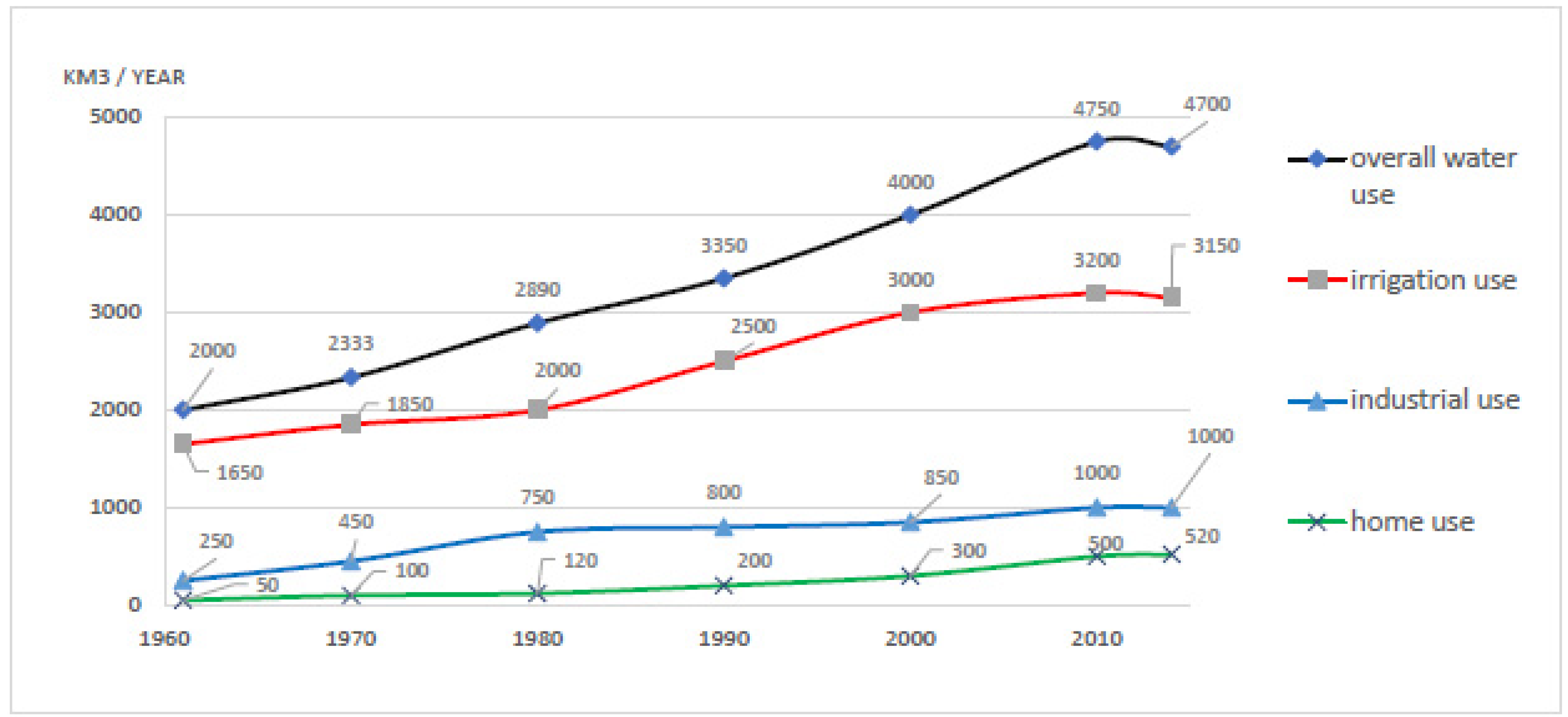
FAO (Food and Agriculture Organization of the United Nations) released the global overview report on agricultural water resources (FAO, 2020/11/26) [1], which pointed out that agricultural water accounts for more than 70%. Figure 1 shows the global distribution of water use from 1961 to 2014, in which irrigation water use has increased year by year, ranking first among all types of water use.

Due to climate change, abnormal high temperatures around the world have led to dwindling freshwater resources. Under the current shortage of water resources, agricultural development will be seriously threatened (Porkka et al., 2016, Rosa et al., 2020) [2,3] and this will indirectly affect human food security (Foley et al., 2011) [4].

China is the world’s second largest economy and a major agricultural country. According to the 2020 National Economic and Social Development Statistical Bulletin of the National Bureau of Statistics of the People’s Republic of China, the annual grain planting area in 2020 was 116.77 million hectares, an increase of 700,000 hectares over the previous year [5]. The annual grain output was 669.49 million tons, an increase of 5.65 million tons or 0.9% over the previous year. He et al. (2019) [6] pointed out that based on the current eating habits of Chinese people, more arable land and irrigation water are needed to help obtain food.

Zongxing et al. (2016) and Sun et al. (2018) [7,8] found that China’s rivers are gradually disappearing under climate change, and Li et al. (2016) and Wang et al. (2019) [9,10] also pointed out that the surviving rivers are also polluted due to economic development. Wang, Y. (2019) and Li et al. (2020) [10,11] also stated that due to China’s industry, urbanization, and population expansion, the area of cultivated land is also gradually decreasing.

Agricultural development is the foundation of national livelihood and economy. As a major food producer, China still faces food shortages. In relation to the 2030 Sustainable Development Goals (Sustainable Development Goals, SDGs) announced by the United Nations in 2015, the second goal is to eliminate hunger and create sustainable food. Additionally, the sixth core goal is providing sanitation and sustainable management of water resources for all. Under extreme climates and limited arable land, how to manage water use to achieve sustainable agricultural development has attracted much attention.

The paper is structured as follows: Section 2 presents the literature review, Section 3 discusses the research methodology, Section 4 presents the empirical analysis, and Section 5 provides conclusions and recommendations. This dossier includes a number of acronyms, which are summarized in

Table 1. Abbreviations used in full.

Abbreviations	Full Name
FAO	Food and Agriculture Organization of the United Nations
SDGs	Sustainable Development Goals
DEA	Date Envelopment Analysis
SBM	Slacks-Based Measure
COD	Chemical Oxygen Demand
GDP	Gross Domestic Product
DMU	Decision Making Unit
IRS	Increasing Return of Scale
DRS	Decreasing Return of Scale
DSBM	Dynamic Slacks-Based Measure
PPS	Possible Production Set

.

2. Literature Review

Cao et al. (2018) and Geng et al. (2019) [12,13] pointed out that improving water efficiency can increase agricultural productivity and is an effective way to solve food shortages. Regarding the measurement of water use efficiency, traditional evaluation methods only consider the relationship between single water use and output GDP. This study believes that to explore the efficiency of agriculture, other variables may need to be evaluated at the same time, which are more objective.

Data envelopment analysis (DEA) is a comprehensive efficiency index that can measure multiple inputs and outputs at the same time, and its results are easy to show performance, so it is accepted by ordinary people.

For example, Bai et al. (2017) [14] applied DEA, input labor, fixed asset investment, water consumption, output GDP, and chemical oxygen demand (COD) to evaluate the water resources, environment, and economic efficiency of the Bohai Bay urban agglomeration in China, and the empirical results show that the efficiency of water resource utilization in the Bohai Bay area has improved, but pollution poses a serious threat to the rapid growth of available water resource protection, and solving the pollution problem is the key to preventing environmental degradation. Hu et al. (2018) [15] applied DEA, input domestic water consumption, industrial and agricultural water consumption, fixed assets, labor force, and GDP of output area, and evaluated the ecological efficiency of China’s water use in 2014. The empirical results show that the overall water environment is poor, and China needs to focus on reducing industrial waste water; there is a lot of room for improvement in water consumption. Yan (2019) [16] evaluated the water use efficiency of 11 cities in Shanxi in 2016. These studies on water use efficiency belong to single-period static analysis.

Since static analysis does not have a vertical link to measure the impact on the next period of efficiency, it is easy to overestimate the efficiency. So, to measure the performance of water efficiency over a period of time, scholars use dynamic analysis for evaluation, such as Sun et al. (2014) [17] who applied the SBM model to explore the influence of external adverse factors on water efficiency; the empirical evidence shows that there is a significant spatial correlation between the output of considering and not considering the adverse factors. Deng et al. (2016) [18] applied the SBM model to explore the influence of external adverse factors on water efficiency; the empirical results show that economically developed administrative regions have higher water efficiency, but lower sewage treatment efficiency. Luo et al. (2018) [19] applied the SBM model, inputting industrial, agricultural, and domestic water consumption and outputting wastewater discharge, and evaluated water use efficiency in 12 provinces and cities in western China; the empirical results show that technological progress has had a positive impact on water use efficiency. Ren et al. (2016) [20] inputted water resource consumption, arable land area, output grain output, livestock quantity, service industry gross production value, and existing research from 2003 to 2013 in Gansu Province (China Urban Water Efficiency).

Another study on the efficiency of water in agriculture, such as the work of Xue and Zhou (2018) [21], applied the SBM model to evaluate the water use efficiency of rice production in China from 2004 to 2014 by inputting fertilizer, water consumption, labor force, planting area, and capital, and using the output as the output. The results showed that the water use efficiency of rice in many regions did not reach the production frontier due to pollution emissions, but the water use efficiency of rice in all regions gradually improved.

Wang et al. (2019) [22] evaluated the efficiency of agricultural water use in China from 2000 to 2015 based on investment capital, labor force, water consumption, net value of agricultural fixed assets, and agricultural output value added. The results showed that the efficiency of agricultural water use in various regions has gradually increased, and with regard to rural residents, the proportion of household per capita disposable income with a high school degree or above is a factor that affects agricultural water use efficiency.

Shi et al. (2020) [23] applied the SBM model, input agricultural water consumption, agricultural employees, arable land area, fixed assets, output agricultural output value, and crop disaster areas, and evaluated the impact of climate change on agricultural production in 30 provinces of China from 2010 to 2017. The results show that China’s agricultural production efficiency is unevenly distributed. The central and eastern regions have the best agricultural production efficiency, while the western regions have low agricultural production efficiency. The distribution difference in agricultural water resources across the country has gradually decreased, but due to extreme weather, agricultural water supply and water-saving measures should be controlled.

Because water use is very important to agricultural production, there are few studies on water use as an exogenous variable of agricultural production. This study observes that the rate of change in China’s agricultural arable land area has been very small in recent years. From the perspective of solving the food problem and sustainable agricultural development, it is not easy to increase the arable land area to increase the production capacity. After summarizing the above-mentioned literature, when discussing the issue of water use efficiency in agriculture, the less-used agricultural land area and variables such as chemical fertilizers are analyzed together.

Based on the discussion of the impact of water use on China’s agriculture, this study took 30 regions in China as the research objects, applied the dynamic SBM model, selected the agricultural labor force and agricultural chemical fertilizers as the inputs, and took agricultural gross domestic product as the single output, using agricultural water use as an external factor and agricultural land area as an immutable intertemporal variable, to measure the impact of China’s water use on agricultural efficiency from 2012 to 2016. In the future, through the empirical results, this work can provide references for relevant government departments in formulating policies to achieve sustainable agricultural development.

3. Methods

3.1. Data Envelopment Analysis (DEA)

Proposed by Farrell (1957) [24], DEA is mainly based on the theory of the boundary production function. After connecting the production set point with the most efficient value into the equal output line, it uses the gap between the production point and the equal output line distributed in the coordinates, and this gap between them represents the degree of efficiency of the production point. In other words, the efficiency frontier formed by the data of input variables and output variables selected by each DMU through the principle of linear programming is called the efficiency index. The relative efficiency of each DMU is determined and evaluated according to the moment distance between the generated distribution points and the efficiency boundary.

Based on Farrell’s theoretical model of economic efficiency, Charnes et al. (1978) [25] extended and improved it into the CCR model to analyze the characteristics of multiple input and output variables under fixed scale returns and to analyze and evaluate the efficiency value. In practice, a DMU may have the situation of increasing returns to scale (IRS) or decreasing returns to scale (DRS). Therefore, Banker et al. (1984) [26] extended and developed the BCC model after the works of Farrell and CCR. This BCC model assumes that the production technology is a variable returns to scale, which can be measured by input orientation or output orientation, and the calculated efficiency values are different. The above three models usually only focus on a separate time period, thus belonging to the realm of static analysis.

3.2. Dynamic Environmental Overall Efficiency Model

Considering the changes over time, a separate time period model is not suitable for long-term performance assessment. Tone and Tsutsui (2010) [27] developed a long-term perspective based on the slacks-based measure (SBM) framework, incorporating carry-over activities into the model; this is called the dynamic slacks-based measure (DN-SBM) model. The model is divided into three types, input, output, and non-oriented, and uses the SBM model proposed by Tone (2001) [28] to find the optimal solution. The variables in this model are also measured using difference variables as the basis, and the SBM efficiency is evaluated in a non-ray mode with a single dataset, with efficiency values ranging from 0 to 1. The efficiency values calculated by this model have two advantages: they do not change depending on the unit of measurement of the input and output variables, and the difference between the input and output decreases over time.

Figure 2 shows the model for this study with n DMUs through time. Each DMU has input and output variables in period t linked to period t + 1 through a carry-over.

The study is based on 30 administrative regions in China, i.e., 30 DMUs (j = 1, …, 30); there are 3 inputs (i = k, l, m) in each of the 30 DMUs, where i is agricultural labor, agricultural fertilizer, and agricultural water, and there is 1 output (j = o) of agricultural GDP; and agricultural arable land area is the carry-over. Since arable land area is a non-controllable factor, the carry-over (fix) non-variable model is used in this study.

The following is a linear programming equation for the basic DSBM model, where PPS is the production set, and θ is the dynamic SBM efficiency value.

$$\begin{gathered} \mathrm{PPS}: \mathrm{T}=\{ ({\mathrm{x}}_{\mathrm{iht}},{ \mathrm{y}}_{\mathrm{jht}} ,{ \mathrm{e}}_{\mathrm{kht}}) | {\mathrm{x}}_{\mathrm{iht} }\ge {{\displaystyle \sum }}_{\mathrm{d}=1}^{\mathrm{n} }{ \mathrm{x}}_{\mathrm{idt}}{ \mathsf{\lambda }}_{\mathrm{d} ,}^{\mathrm{t}} ( \mathrm{i}=1, 2, \dots \mathrm{m}; \mathrm{d}=1, 2, \dots \mathrm{n} ; \mathrm{t}=1,2,\dots \mathrm{T}), \\ { \mathrm{y}}_{\mathrm{iht} }\le {{\displaystyle \sum }}_{\mathrm{d}=1}^{\mathrm{n}}{ \mathrm{y}}_{\mathrm{idt} }{\mathsf{\lambda }}_{\mathrm{d} }^{\mathrm{t}}( \mathrm{j}=1, 2, \dots \mathrm{o}; \mathrm{d}=1, 2, \dots \mathrm{n} ; \mathrm{t}=1,2,\dots \mathrm{T}) \} \end{gathered}$$

(1)

$$\begin{array}{l}{\mathrm{z} }_{\ell \mathrm{dt} }^{\mathrm{bad}}\le {{\displaystyle \sum }}_{\mathrm{d}=1}^{\mathrm{n}}{ \mathrm{z}}_{ \ell \mathrm{dt} }^{ \mathrm{bad}}{ \mathsf{\lambda }}_{\mathrm{d} ,}^{\mathrm{t} } ( \mathrm{d}=1, 2 \dots \mathrm{n}; \ell =1, 2\dots \mathrm{q}; \mathrm{t}=1, 2, \dots \mathrm{T}) \\ { \mathsf{\lambda }}_{\mathrm{d} }^{\mathrm{t}}\ge 0,( \mathrm{d}=1, \dots , \mathrm{n}; \mathrm{t}=1, \dots , 7) \\ {{\displaystyle \sum }}_{\mathrm{d}=1}^{\mathrm{n} }{\mathsf{\lambda } }_{\mathrm{d} }^{\mathrm{t}}=1,(\mathrm{t}=1, \dots , \mathrm{T}) \end{array}$$

The equation below is mathematical and satisfies the inter-period variability condition from period t to period t + 1 and is an important constraint on DSBM activity linking period t to period t + 1. Here, α in (2) can be expressed as good.

$${{\displaystyle \sum }}_{\mathrm{j}=1}^{\mathrm{n}}{\mathrm{z}}_{\mathrm{ijt} }^{\mathsf{\alpha }}{\mathsf{\lambda }}_{\mathrm{j} }^{\mathrm{t}}={{\displaystyle \sum }}_{\mathrm{j}=1}^{\mathrm{n}}{\mathrm{z}}_{\mathrm{ijt} }^{\mathsf{\alpha }}{\mathsf{\lambda }}_{\mathrm{j} }^{\mathrm{t}+1} ,\forall \mathrm{i} ; (\mathrm{t}=1, \dots , \mathrm{T}-1 )$$

(2)

• x: inputs (i = k, l, m);
• y: outputs (j = o);
• z: carry-over connected to agricultural arable land area (ℓ = 1, 2, …, q).

$${\mathsf{\theta }}_{\mathrm{dt}}^{*}=\min \frac{\frac{1}{\mathrm{T}}{{\displaystyle \sum }}_{\mathrm{t}=1}^{\mathrm{T}=7}{\mathrm{w}}^{\mathrm{t}}\left[1-\frac{1}{\mathrm{m}+\mathrm{p}}\left({{\displaystyle \sum }}_{\mathrm{i}=1}^{\mathrm{m}}\frac{{\mathrm{w}}_{\mathrm{i}}^{-}{\mathrm{s}}_{\mathrm{it}}^{-}}{{\mathrm{x}}_{\mathrm{iht}}}\right)\right]}{\frac{1}{\mathrm{T}}{{\displaystyle \sum }}_{\mathrm{t}=1}^{\mathrm{T}=7}{\mathrm{w}}^{\mathrm{t}}\left[1+\frac{1}{\mathrm{o}+\mathrm{q}}\left({{\displaystyle \sum }}_{\mathrm{j}=1}^{\mathrm{o}}\frac{{\mathrm{w}}_{\mathrm{j}}^{+}{\mathrm{s}}_{\mathrm{jt}}^{+}}{{\mathrm{y}}_{\mathrm{jht}}}+{{\displaystyle \sum }}_{\ell =1}^{\mathrm{q}}\frac{{\mathrm{s}}_{\mathrm{lt}}^{+\mathrm{bad}}}{{ \mathrm{z}}_{\mathrm{lht}}{}^{\mathrm{bad}}} \right)\right]}$$

$$= \min \frac{{{\displaystyle \sum }}_{\mathrm{t}=1}^{\mathrm{T}=7}{\mathrm{w}}^{\mathrm{t}}\left[ 1-\frac{1}{\mathrm{m}+\mathrm{p} } \left({{\displaystyle \sum }}_{\mathrm{i}=1}^{\mathrm{m}}\frac{{ \mathrm{w}}_{\mathrm{i}}^{-}{\mathrm{s}}_{\mathrm{it}}^{-}}{{\mathrm{x}}_{\mathrm{iht}}}\right)\right]}{{{\displaystyle \sum }}_{\mathrm{t}=1}^{\mathrm{T}=7}{\mathrm{w}}^{\mathrm{t}}\left[ 1+\frac{1}{\mathrm{o}+\mathrm{q}}\left({{\displaystyle \sum }}_{\mathrm{j}=1}^0\frac{{\mathrm{w}}_{\mathrm{j}}^{+}{\mathrm{s}}_{\mathrm{jt}}^{+}}{{\mathrm{y}}_{\mathrm{jht}}}+{{\displaystyle \sum }}_{\ell =1}^{\mathrm{q}}\frac{{ \mathrm{s}}_{\ell \mathrm{t}}^{+\mathrm{bad}}}{{ \mathrm{z}}_{\ell \mathrm{ht}}{}^{\mathrm{bad}}}\right)\right]}$$

(3)

$$\mathrm{S}.\mathrm{t}.$$

$$\begin{array}{l}{\mathrm{x}}_{\mathrm{iht}}={\displaystyle {\displaystyle \sum }_{\mathrm{d}=1}^{\mathrm{n} }}{ \mathrm{x}}_{\mathrm{idt}}{ \mathsf{\lambda }}_{\mathrm{d} }^{\mathrm{t}}+{\mathrm{s}}_{\mathrm{it}}^{-},\left(\mathrm{i}=1,2,\dots ,\mathrm{m};\mathrm{d}=1,2,\dots ,\mathrm{n}; \mathrm{t}=1,2,\dots ,5\right) \\ {\mathrm{y}}_{\mathrm{jht}}\le {{\displaystyle \sum }}_{\mathrm{d}=1}^{\mathrm{n}}{\mathrm{y}}_{\mathrm{jdt}}{\ast \mathsf{\lambda }}_{\mathrm{d}}^{\mathrm{t}}+{\mathrm{s}}_{\mathrm{jt}}^{-}, (\mathrm{j}=1,2,\dots ,\mathrm{o}; \mathrm{d}=1,2,\dots ,\mathrm{n}; \mathrm{t}=1,2,\dots ,5)\\ {\mathrm{z}}_{\ell \mathrm{dt}}^{\mathrm{bad}}={\displaystyle {\displaystyle \sum }_{\mathrm{d}=1}^{\mathrm{n}}}{\mathrm{z}}_{\ell \mathrm{dt}}^{\mathrm{bad}}{\mathsf{\lambda }}_{\mathrm{d}}^{\mathrm{t}}+{\mathrm{s}}_{\ell \mathrm{t}}^{\mathrm{bad}},\left(\ell =1,2,\dots ,\mathrm{q};\mathrm{d}=1,\dots ,\mathrm{n} ;\mathrm{t}=1,2,\dots ,5\right)\\ {{\displaystyle \sum }}_{\mathrm{d}=1}^{\mathrm{n}}{ \mathsf{\lambda }}_{\mathrm{j}}^{\mathrm{t}}=1,\left(\mathrm{d} =1,\dots , \mathrm{n}; \mathrm{t} =1,2,\dots , 5\right) \mathrm{VRS}\end{array}$$

$${\lambda }_{\mathrm{d}}^{\mathrm{t}}\ge 0 ,{ \mathrm{s}}_{\mathrm{it}}^{-}\ge 0,{ \mathrm{s}}_{\mathrm{jt}}^{+}\ge 0,{ \mathrm{s}}_{\ell \mathrm{t}}^{\mathrm{bad}}\ge 0 ,$$

(4)

The most efficient value available (overall efficiency of the dynamic environment) is as follows:

$${\mathsf{\theta }}_{\mathrm{ht}}=\frac{1-\frac{1}{\mathrm{m} + \mathrm{p} }\left({{\displaystyle \sum }}_{\mathrm{i}=1}^{\mathrm{m}}\frac{{\mathrm{w}}_{\mathrm{i}}^{-}{\mathrm{s}}_{\mathrm{it} }^{-}}{{\mathrm{x}}_{\mathrm{iht}}}\right)}{1+\frac{1}{\mathrm{o} + \mathrm{q}}\left({{\displaystyle \sum }}_{\mathrm{i}=1}^{\mathrm{o}}\frac{{\mathrm{w}}_{\mathrm{j}}^{+}{\mathrm{s}}_{\mathrm{jt}}^{+}}{{\mathrm{y}}_{\mathrm{jht}}}\right)}\left(\mathrm{t}=1,\dots ,7\right)$$

(5)

Equations (3)–(5) represent a multi-period dynamic agricultural efficiency measurement model for the 30 administrative regions in China.

4. Results

We applied a dynamic SBM model to measure the impact of water resources on agricultural efficiency in China. We based this on the completeness and availability of research data collected, using 30 administrative regions in China over the period of 2012–2016 and collecting all of the data from the National Bureau of Statistics of China. We selected agricultural labor and fertilizer as the input variables, gross domestic product (GDP) in agriculture as a single output variable, arable land area as a non-variable inter-period variable, and irrigation water in agriculture as an exogenous variable.

Table 2. Descriptions of the variables included.

Selection of Variables		Unit	Description	Expected Trend
Inputs	Agricultural labor	people	Population over 16 years of age involved in agricultural activities.	Down
	Agricultural fertilizer	ton	Refers to the amount of fertilizer actually used in agricultural production.	Down
	Water for agriculture	m3	Water used for irrigation of agricultural land, irrigation of forest and fruit land, irrigation of grassland, and recharge of fish ponds.	Down
Output	Agricultural GDP	RMB	It is based on the production of agricultural products and their by-products multiplied by the price per unit of product.	Up
Carry-over	Arable land area	hectare	Area of land that has been reclaimed for growing crops and is regularly cultivated.	Non-controllable

Note: Data source: own compilation.

presents a description of the input, output, and inter-period variables

4.1. Statistical Analysis

Table 3. Input and output statistics: 2012 to 2016.

Variable	Mean	Max.	Min.	St. Dev.
Agricultural labor (M peoples)	9.211	26.517	0.448	6.449
Agricultural fertilizers (M tons)	1.98	7.16	0.0876	1.49
Agricultural water (B m3)	12.784	56.17	0.6	11.038
Agricultural GDP (B RMB)	170.14	466.261	11.709	116.301
Cultivated area (sq. km)	54.864	148.797	1.209	38.943

Note: Data source: own compilation.

shows the overall input and output variable statistics for the 30 administrative regions of the country of China from 2013 to 2016. The maximum value of labor force in agriculture is Henan in 2014 and the minimum value is Shanghai in 2014. The maximum value of chemical fertilizer in agriculture is Henan in 2015 and the minimum value is Qinghai in 2016. The maximum value of water use in agriculture is Xinjiang Uygur Autonomous Region in 2012, and the minimum value is Shanghai in 2016. The maximum value of agriculture is Shandong in 2015, and the minimum value is Qinghai in 2012. The maximum value of arable land area is Henan in 2015, and the minimum value is Beijing in 2016.

According to

Table 4. Means and trend scenarios for each variable in each year.

Variable	2012	2013	2014	2015	2016	Average	Diff. (%)
Agricultural labor (M peoples)	9.52	9.34	9.20	9.05	8.95	9.21	−6.00%
Agricultural fertilizers (M tons)	1.95	1.97	2.00	2.01	1.99	1.98	2.47%
Agricultural water (B m3)	12.92	12.98	12.80	12.75	12.47	12.78	−3.48%
Agricultural GDP (B RMB)	149.31	162.95	172.63	180.46	185.36	243.79	24.15%
Cultivated area (sq. km)	53.95	54.49	54.99	55.53	55.36	54.86	2.61%

Note: Data source: own compilation.

, the agricultural labor force in China has been decreasing year on year during the study period, with an overall decrease of 6.0%, while the highest and lowest average values are 9.52 M peoples in 2012 and 8.95 M peoples in 2016. The overall increase in agricultural fertilizer was 2.47%, with the highest and lowest average values being 2.01 M tons in 2015 and 1.95 M tons in 2012. Agricultural water use as a whole decreased by 3.48%, with the highest and lowest average values being 12.980 B m³ in 2013 and 12.47 B m³ in 2016. Single output agricultural GDP, on the other hand, showed a year-on-year increase of 24.15% overall, with little variation in the area of arable land by year, but it was also up by 2.61%.

4.2. Efficiency Analysis

4.2.1. Agricultural Efficiency

The results (

Table 5. Agricultural efficiency performance in China’s 30 administrative regions.

DMU	Efficiency without Water							Efficiency of Water Resources
	2012	2013	2014	2015	2016	Overall Score	Rank	2012	2013	2014	2015	2016	Overall Score	Rank
Beijing	1	1	1	1	1	1	1	1	1	1	1	1	1	1
Tianjin	0.527	0.686	1	1	1	0.831	16	1	1	1	1	1	1	1
Hebei Province	0.777	0.820	0.715	0.9990	0.590	0.769	17	1	1	0.961	1	0.818	0.952	21
Shanxi Province	0.521	1.000	0.471	1	0.418	0.612	27	0.757	0.999	0.703	1	0.581	0.775	24
Inner Mongolia Autonomous Region	0.675	0.621	0.622	1	1	0.757	19	1	1	1	1	1	1	1
Liaoning Province	0.819	0.842	0.754	1	0.818	0.846	15	0.989	0.916	0.897	1	0.985	0.957	20
Jilin Province	0.549	1	0.528	0.452	0.405	0.544	29	1	1	1	1	1	1	1
Heilongjiang Province	1	1	1	1	1	1	1	1	1	1	1	1	1	1
Shanghai	1	1	1	1	1	1	1	1	1	1	1	1	1	1
Jiangsu Province	1	1	1	1	1	1	1	1	1	1	1	1	1	1
Zhejiang Province	1	1	1	1	1	1	1	1	1	1	1	1	1	1
Anhui Province	0.494	0.999	0.464	0.513	1	0.639	23	0.627	0.999	0.596	0.572	1	0.713	26
Fujian Province	1	1	1	1	1	1	1	1	1	1	1	1	1	1
Jiangxi Province	0.562	0.652	0.524	0.894	0.62	0.636	24	0.59	0.58	0.541	0.788	0.66	0.621	29
Shandong Province	0.999	1	1	1	0.999	1	1	1	1	1	1	1	1	1
Henan Province	0.999	0.999	0.999	0.999	0.999	0.999	12	1	1	1	1	1	1	1
Hubei Province	0.621	0.62	0.582	0.67	0.599	0.618	26	0.753	0.77	0.723	0.921	0.815	0.792	22
Hunan Province	0.711	0.767	0.656	1	0.603	0.74	20	0.806	0.743	0.7	1	0.688	0.779	23
Guangdong Province	0.999	1	1	0.999	0.999	0.999	11	0.999	0.999	1	0.999	1	0.999	18
Guangxi Zhuang Autonomous Region	0.573	0.535	1	1	0.566	0.71	21	0.6	0.588	1	1	0.644	0.744	25
Hainan	0.792	1	1	1	1	0.958	13	0.838	1	1	1	1	0.967	19
Chongqing	0.624	0.704	0.68	0.658	0.738	0.679	22	1	1	1	1	1	1	1
Sichuan Province	1	1	1	1	1	1	1	1	1	1	1	1	1	1
Guizhou Province	0.551	1	1	1	1	0.897	14	1	1	1	1	1	1	1
Yunnan Province	0.462	0.638	0.556	0.692	0.449	0.559	28	0.623	0.673	0.684	0.999	0.606	0.7	27
Shaanxi Province	0.638	1	0.755	0.754	0.666	0.759	18	1	1	1	1	1	1	1
Gansu province	0.532	0.997	0.53	0.672	0.516	0.629	25	0.616	0.996	0.582	0.583	0.578	0.65	28
Qinghai Province	1	1	1	1	1	1	1	1	1	1	1	1	1	1
Ningxia Hui Autonomous Region	0.45	0.572	0.478	0.58	0.557	0.527	30	0.441	0.474	0.432	0.503	0.506	0.469	30
Xinjiang Uygur Autonomous Region	1	1	1	1	1	1	1	1	1	1	1	1	1	1
Average	0.762	0.881	0.81	0.896	0.818	0.823		0.888	0.924	0.894	0.945	0.896	0.904

Note: Data source: compiled by this study.

) show that the annual efficiency and overall efficiency of agriculture excluding agricultural water in the 30 administrative regions of China from 2012 to 2016 are 0.834. The average annual efficiency of each sub-region was maintained between 0.763 and 0.896, with the efficiency of 2013 and 2015 being higher than average, which was the best performing year.

The efficiency values of 10 administrative regions, including Beijing, Heilongjiang, Shanghai, Jiangsu, Zhejiang, Fujian, Shandong, Sichuan, Qinghai, and Xinjiang, are at the forefront of efficiency and have the best agricultural efficiency performance. The efficiency values of six administrative regions, including Tianjin, Liaoning, Guangdong, Henan, Hainan, and Guizhou, are above the level of 0.834, but are not at 1. The efficiencies of Guangdong and Henan remain stable at 0.999. In addition, 14 regions, including Hebei, Shanxi, Inner Mongolia, Jilin, Anhui, Jiangxi, Hubei, Hunan, Guangxi, Chongqing, Yunnan, Shaanxi, Gansu, and Ningxia (see Figure 3), are below the level of efficiency, of which Yunnan (0.5598), Jilin (0.5449), and Ningxia (0.5275) have the lowest efficiency.

During the five-year period, the annual efficiencies of Tianjin were 0.527, 0.686, 1, 1, and 1, respectively, and the overall efficiency increased by 89.75%, indicating that Tianjin adopted effective resource allocation to improve efficiency. In addition, the annual efficiencies of Jilin were 0.549, 1, 0.528, 0.452, and 0.405. Except for the best resource allocation in 2013, the resource allocation in the other years did not improve significantly, and so it has a lot of room to adjust resource allocation to improve agricultural efficiency. The overall efficiency of China’s agriculture after the input of agricultural water is 0.910, and the average annual efficiency value of each sub-point is between 0.88 and 0.946. Its overall efficiency and annual efficiency are better than the efficiency performance of unused agricultural water. The overall efficiency values of 17 administrative regions, including Beijing, Tianjin, Inner Mongolia, Jilin, Heilongjiang, Shanghai, Jiangsu, Zhejiang, Fujian, Shandong, Henan, Chongqing, Sichuan, Guizhou, Shaanxi, Qinghai, and Xinjiang, are at the forefront of efficiency, and they have the best agricultural efficiency performance (see Figure 4).

The efficiency values of four administrative regions, including Guangdong, Hainan, Liaoning, and Hebei, are higher than the level of 0.910, whereby Hainan increased its efficiency by 19.33% in 2016 compared with 2012, indicating that the province’s effective management of resource allocation has improved. In addition, there are nine administrative regions with lower efficiency values: Shanxi, Hubei, Hunan, Guangxi, Anhui, Yunnan, Gansu, Jiangxi, and Ningxia, of which Gansu (0.671), Jiangxi (0.632), and Ningxia (0.471) are the least efficient administrative regions. The annual efficiency of Gansu has decreased by 6.17%, showing that there has been no improvement in resource allocation.

4.2.2. Sensitivity Analysis

From Figure 5, we can see that the difference in agricultural efficiency in China between 2012 and 2016 is better than that of the annual rate after agricultural water was used (0.888, 0.925, 0.894, 0.946, and 0.896, respectively), which was better than the efficiency of unused agricultural water (0.763, 0.882, 0.811, 0.896, and 0.818, respectively).

After the input of agricultural water, the overall average efficiency of agriculture increased from 0.834 to 0.910. The overall efficiency value of the 10 administrative regions of Beijing, Heilongjiang, Shanghai, Jiangsu, Zhejiang, Fujian, Shandong, Sichuan, Qinghai, and Xinjiang has always been 1, and their efficiency performance is not affected by agricultural water use. They still have the best agricultural efficiency performance (see Appendix A).

After the input of agricultural water, the agricultural efficiency of the 17 administrative regions of Tianjin, Hebei, Shanxi, Inner Mongolia, Liaoning, Jilin, Anhui, Henan, Hubei, Hunan, Guangxi, Hainan, Chongqing, Guizhou, Yunnan, Shaanxi, and Gansu was seen to have increased. The agricultural efficiency value of Jilin rose from 0.545 to 1, or an increase of 83.52%, and Chongqing, Inner Mongolia, Shaanxi, and Hubei also increased by 47.21%, 32.10%, 31.72%, and 28.15%. They are the five administrative districts with the most efficiency gains, indicating that agricultural water use is positive for their efficiency. However, the agricultural efficiency of Jiangxi and Ningxia declined by 2.42% and 10.49%, and it is necessary to manage agricultural water in particular to improve their overall efficiency of agriculture (see Figure 6).

4.2.3. Adjust the Margin Range

We forecasted the adjustment balance of the total factors measuring China’s agricultural efficiency from 2012 to 2016 (see Appendix B). The adjustment range is the difference in the effective boundary between input and output variables. When the adjustment rate is 0, it means that input or output does not need to be changed. When the adjustment range is greater than 0, it indicates that input or output should be increased. Conversely, when the adjustment range is less than 0, it means that the input or output should be reduced.

According to the results, from 2012 to 2016, the agricultural labor force, agricultural fertilizer, agricultural water, and agricultural GDP of 30 administrative regions in China needed to be reduced by 2.651%, 1.099%, 6.258%, and 9.685% on average. The 16 administrative regions of Beijing, Tianjin, Inner Mongolia, Jilin, Heilongjiang, Shanghai, Jiangsu, Zhejiang, Fujian, Shandong, Henan, Chongqing, Guizhou, Shaanxi, Qinghai, and Xinjiang do not need to adjust their variables. The input and output variables of Hebei, Shanxi, Liaoning, Anhui, Jiangxi, Hubei, Hunan, Guangdong, Guangxi, Hainan, Sichuan, Yunnan, Gansu, and Ningxia all need to be adjusted (see Figure 7).

In terms of input, the three regions with the worst agricultural labor efficiency are Gansu, Jiangxi, and Yunnan, which need to reduce their input by 18.132%, 14.368%, and 13.924%, respectively. The three administrative regions with the worst agricultural fertilizer efficiency are Hubei, Ningxia, and Hebei, which need to reduce their input by 9.668%, −8.442%, and 5.280%, respectively. The three regions with the worst agricultural water use efficiency are Ningxia, Guangxi, and Hunan, which need to reduce their input by 44.386%, 26.304, and 25.112%, respectively. Ningxia, Jiangxi, and Anhui are the three regions with the worst efficiency in agricultural output and need to increase their output by 74.144%, 43.818%, and 39.406%, respectively.

On the whole, excessive agricultural water consumption and insufficient agricultural output are the reasons affecting agricultural efficiency. Jiangxi and Ningxia should not only manage agricultural water consumption, but also increase agricultural output value to improve their overall agricultural efficiency.

5. Conclusions and Suggestions

5.1. Conclusions

This research takes agricultural water as an exogenous variable to analyze the agricultural efficiency of 30 administrative regions in China and further examines the sensitivity and suggests an adjustment range.

The average changes of input and output variables from 2012 to 2016 are summarized in Appendix C. The policy implications for the 30 administrative regions in China are as follows.

(1)

The average value of agricultural water use efficiency without agricultural water use is 0.834, and the average value of agricultural water use efficiency with agricultural water use is 0.910, indicating that agricultural water use does affect the overall performance of agricultural efficiency.

(2)

From 2012 to 2016, the efficiency of agricultural production in Jiangxi and Ningxia changed from high to low after the input of agricultural water. This means that these two regions need to effectively manage water resources and adjust their utilization to improve efficiency.

(3)

During the study period, the labor force in agriculture decreased by 5.99%, and the fertilizer increased by 2.48%. The total area of arable land increased by 2.61%, water consumption decreased by 3.48%, and the gross production value increased by 24.14%. The empirical results of this study show that agriculture in all administrative regions of China is moving forward toward the policy implementation goals.

(4)

We forecasted the adjustment range of China’s agricultural efficiency from 2012 to 2016, such as a 2.651% reduction in agricultural labor force, a 1.099% reduction in agricultural fertilizer, a 6.258% reduction in agricultural water, and a 9.685% increase in agricultural GDP. It can be seen that excessive agricultural water use and insufficient agricultural output are the reasons affecting agricultural efficiency, indicating that there is still room for efforts in the effective utilization of agricultural irrigation water in the 12th five-year water conservancy reform and development goal.

(5)

Overall, the utilization of agricultural water resources in China presents a trend toward higher efficiency, but in the face of more severe natural environment changes in the future, existing resources should be used more carefully to make water resources more beneficial to agricultural production efficiency. In particular, Jiangxi and Ningxia, which are severely short of water in north China, went from having a high efficiency value to a low efficiency value after adding agricultural water into the non-agricultural production efficiency variable from 2012 to 2016. Therefore, better management is needed to improve the efficiency of agricultural water resources.

5.2. Suggestions

This study took China as the research object and collected all quantifiable information from the National Bureau of Statistics of China, but the difficulty of collecting data on relevant variables led to limitations in the study. In the future, scholars can further refine and add variables related to external impacts on water into the discussion, extend the research time, cover a greater time period, or use other research methods for evaluation to make the evidence more complete.

References

1. The State of World Fisheries and Aquaculture 2022; FAO: Rome, Italy, 2022. [CrossRef]
2. Porkka, M.; Gerten, D.; Schaphoff, S.; Siebert, S.; Kummu, M. Causes and Trends of Water Scarcity in Food Production. Environ. Res. Lett. 2016, 11, 015001. [Google Scholar] [CrossRef] [Green Version]
3. Rosa, L.; Chiarelli, D.D.; Rulli, M.C.; Dell’Angelo, J.; D’Odorico, P. Global Agricultural Economic Water Scarcity. Sci. Adv. 2020, 6, eaaz6031. [Google Scholar] [CrossRef] [PubMed]
4. Foley, J.A.; Ramankutty, N.; Brauman, K.A.; Cassidy, E.S.; Gerber, J.S.; Johnston, M.; Mueller, N.D.; O’Connell, C.; Ray, D.K.; West, P.C.; et al. Solutions for a Cultivated Planet. Nature 2011, 478, 337–342. [Google Scholar] [CrossRef] [PubMed] [Green Version]
5. National Bureau of Statistics of China. Available online: http://www.stats.gov.cn/tjsj/zxfb/202102/t20210227_1814154.html (accessed on 10 February 2023).
6. He, G.; Zhao, Y.; Wang, L.; Jiang, S.; Zhu, Y. China’s Food Security Challenge: Effects of Food Habit Changes on Requirements for Arable Land and Water. J. Clean. Prod. 2019, 229, 739–750. [Google Scholar] [CrossRef]
7. Li, Z.; Qi, F.; Wang, Q.J.; Song, Y.; Cheng, A.; Li, J. Contribution from Frozen Soil Meltwater to Runoff in an In-Land River Basin under Water Scarcity by Isotopic Tracing in Northwestern China. Glob. Planet. Chang. 2016, 136, 41–51. [Google Scholar] [CrossRef]
8. Sun, M.; Liu, S.; Yao, X.; Guo, W.; Xu, J. Glacier Changes in the Qilian Mountains in the Past Half-Century: Based on the Revised First and Second Chinese Glacier Inventory. J. Geogr. Sci. 2018, 28, 206–220. [Google Scholar] [CrossRef] [Green Version]
9. Li, X.; Liu, J.; Zheng, C.; Han, G.; Hoff, H. Energy for Water Utilization in China and Policy Implications for Integrated Planning. Int. J. Water Resour. Dev. 2016, 32, 477–494. [Google Scholar] [CrossRef]
10. Wang, Y. The Challenges and Strategies of Food Security under Rapid Urbanization in China. Sustainability 2019, 11, 542. [Google Scholar] [CrossRef] [Green Version]
11. Li, W.; Hai, X.; Han, L.; Mao, J.; Tian, M. Does Urbanization Intensify Regional Water Scarcity? Evidence and Implications from a Megaregion of China. J. Clean. Prod. 2020, 244, 118592. [Google Scholar] [CrossRef]
12. Cao, X.; Ren, J.; Wu, M.; Guo, X.; Wang, W. Assessing Agricultural Water Use Effect of China Based on Water Footprint Framework. Trans. Chin. Soc. Agric. Eng. 2018, 34, 1–8. [Google Scholar]
13. Geng, Q.; Ren, Q.; Nolan, R.H.; Wu, P.; Yu, Q. Assessing China’s Agricultural Water Use Efficiency in a Green-Blue Water Perspective: A Study Based on Data Envelopment Analysis. Ecol. Indic. 2019, 96, 329–335. [Google Scholar] [CrossRef]
14. Bai, M.; Zhou, S.; Zhao, M.; Yu, J. Water Use Efficiency Improvement against a Backdrop of Expanding City Agglomeration in Developing Countries—A Case Study on Industrial and Agricultural Water Use in the Bohai Bay Region of China. Water 2017, 9, 89. [Google Scholar] [CrossRef] [Green Version]
15. Hu, P.; Chen, N.; Li, Y.; Xie, Q. Efficiency Evaluation of Water Consumption in a Chinese Province-Level Region Based on Data Envelopment Analysis. Water 2018, 10, 793. [Google Scholar] [CrossRef] [Green Version]
16. Yan, J. Spatiotemporal Analysis for Investment Efficiency of China’s Rural Water Conservancy Based on DEA Model and Malmquist Productivity Index Model. Sustain. Comput. Inform. Syst. 2019, 21, 56–71. [Google Scholar] [CrossRef]
17. Sun, C.; Zhao, L.; Zou, W.; Zheng, D. Water Resource Utilization Efficiency and Spatial Spillover Effects in China. J. Geogr. Sci. 2014, 24, 771–788. [Google Scholar] [CrossRef] [Green Version]
18. Deng, G.; Li, L.; Song, Y. Provincial Water Use Efficiency Measurement and Factor Analysis in China: Based on SBM-DEA Model. Ecol. Indic. 2016, 69, 12–18. [Google Scholar] [CrossRef]
19. Luo, Y.; Yin, L.; Qin, Y.; Wang, Z.; Gong, Y. Evaluating Water Use Efficiency in China’s Western Provinces Based on a Slacks-Based Measure (SBM)-Undesirable Window Model and a Malmquist Productivity Index. Symmetry 2018, 10, 301. [Google Scholar] [CrossRef] [Green Version]
20. Ren, C.; Guo, P.; Yang, G.; Li, R.; Liu, L. Spatial and Temporal Analyses of Water Resources Use Efficiency Based on Data Envelope Analysis and Malmquist Index: Case Study in Gansu Province, China. J. Water Resour. Plan. Manag. 2016, 142, 04016066. [Google Scholar] [CrossRef]
21. Xue, C.; Zhou, H. Analysis on Rice Production Water Use Efficiency and Its Influencing Factors in China under Constraint of Pollutant Emission. Water Resour. Prot. 2018, 34, 52–56. [Google Scholar]
22. Wang, F.; Yu, C.; Xiong, L.; Chang, Y. How Can Agricultural Water Use Efficiency Be Promoted in China? A Spatial-Temporal Analysis. Resour. Conserv. Recycl. 2019, 145, 411–418. [Google Scholar] [CrossRef]
23. Shi, Z.; Huang, H.; Wu, Y.; Chiu, Y.-H.; Qin, S. Climate Change Impacts on Agricultural Production and Crop Disaster Area in China. Int. J. Environ. Res. Public Health 2020, 17, 4792. [Google Scholar] [CrossRef]
24. Farrell, M.J. The Measurement of Productive Efficiency. J. R. Stat. Soc. Ser. A 1957, 120, 253–281. [Google Scholar] [CrossRef]
25. Charnes, A.; Cooper, W.W.; Rhodes, E. Measuring the Efficiency of Decision Making Units. Eur. J. Oper. Res. 1978, 2, 429–444. [Google Scholar] [CrossRef]
26. Banker, R.D.; Charnes, A.; Cooper, W.W. Some Models for Estimating Technical and Scale Inefficiencies in Data Envelopment Analysis. Manag. Sci. 1984, 30, 1078–1092. [Google Scholar] [CrossRef] [Green Version]
27. Tone, K.; Tsutsui, M. Dynamic DEA: A Slacks-Based Measure Approach. Omega 2010, 38, 145–156. [Google Scholar] [CrossRef] [Green Version]
28. Tone, K. A Slacks-Based Measure of Efficiency in Data Envelopment Analysis. Eur. J. Oper. Res. 2001, 130, 498–509. [Google Scholar] [CrossRef] [Green Version]
Figure 1. Distribution of global water resources from 1961 to 2014.
Water 15 01266 g001
Figure 2. Dynamic SBM basic model of this study.
Water 15 01266 g002
Figure 3. Efficiency without water.
Water 15 01266 g003
Figure 4. Efficiency of water utilization.
Water 15 01266 g004
Figure 5. Differences in agricultural efficiency in China. Data source: compiled by this study.
Water 15 01266 g005
Figure 6. Sensitivity scenarios for water use efficiency.
Water 15 01266 g006
Figure 7. Areas where inputs and outputs need to be adjusted.
Water 15 01266 g007