Aquaculture Production in the Midst of GHG Emissions in South Africa

Abstract

The study ascertained the relationship between aquaculture production and greenhouse gas (GHG) emissions in South Africa. The study used the Autoregressive Distributed Lag—Error Correction Model (ARDL-VECM) with time series data between 1990 and 2020. The results showed that the mean annual aquaculture production, GHG emissions, and Gross Domestic Product (GDP) in the period were 5200 tonnes, 412 tonnes, and US$447 billion, respectively. There was a long-run relationship between GHG emissions and GDP. In the short run, GHG emissions had a positive relationship with GDP and a negative relationship with beef production. Furthermore, there was a bi-directional relationship between aquaculture production and GHG emissions. In addition, beef production and GDP had a bi-directional relationship. Beef production also had a positive relationship with aquaculture production. The study concludes that aquaculture production is affected and tends to affect GHG emissions. Aquaculture legislation should consider GHG emissions in South Africa and promote sustainable production techniques.

1. Introduction

Aquaculture is an emerging farming method primarily aimed at meeting the growing consumer demand for meat and animal products [1]. It is defined as the process of farming aquatic organisms such as fish, crustaceans, molluscs, and aquatic plants [2]. At the same time, it is a preservation method aimed at protecting various aquatic species from endangerment due to rising poaching rates and seawater pollution. The farming process involves stocking, feeding, and providing protection from predators. South Africa has environmental conditions conducive to aquaculture development and opportunities for commercial production [3], and contributions to local economic and human development, food security, and livelihoods. It is the youngest farming sector in the country, and since 2013, aquaculture production has increased by 75% to 6000 tonnes, managing an R1 billion total value of sales in 2018. However, others have reported a sector value of R8 billion per year, generating more than R3.4 billion in total foreign exchange from sales [4]. The South African aquaculture sector contributes less than 1% to the country’s GDP, 4% to the country’s agricultural GDP, and 5% to Western Cape Province’s GDP [5,6]. A report by WWF-SA [7] highlighted that 500,000 people participated in South Africa’s recreational fishing, with a value of up to R3 billion in 2011.

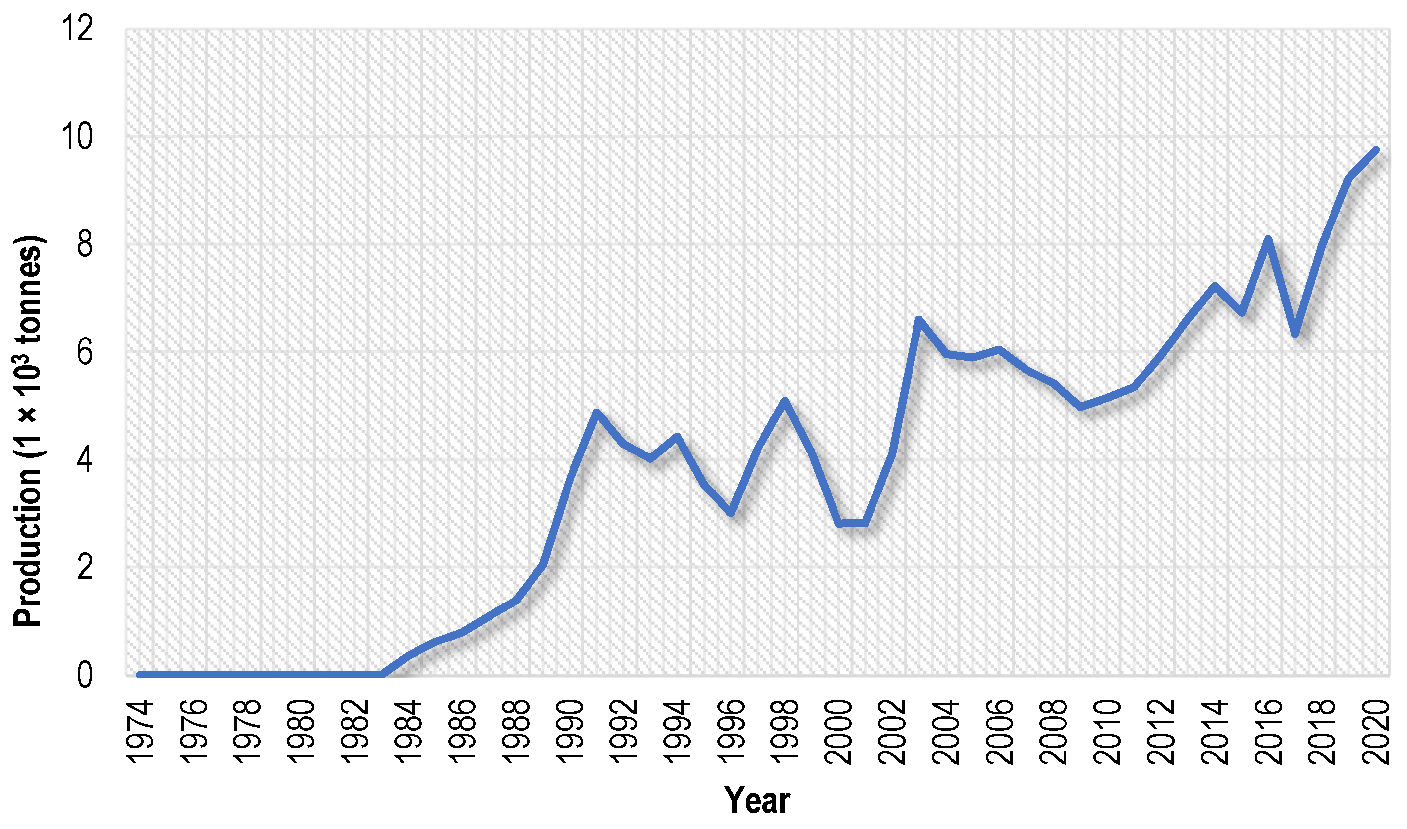
In South Africa, the sector is dominated by abalone (70%), trout (10%) and mussel (6%), acting as a supplement to the wild fishing sector [4]. In 2019, the country’s captured fish and aquaculture production was at 452,900 tonnes consisting of 96% marine fish, 3% molluscs and 0.4% crustaceans, respectively [2]. Figure 1 shows a gradual increase in the trend of aquaculture production in South Africa from 2000 to 2019 [2,8].

The favourable environment in South Africa’s aquaculture industry includes good infrastructure, business institutions, supply chains, and a supportive aquaculture legislation framework. The country’s annual per capita fish consumption is 6–8 kg, with local consumption unable to absorb all production. This allowed international trade, which had a lot of entry barriers such as regulatory compliance, biosecurity guidelines and skills development [4]. To align with national policies such as the National Development Plan (NDP), the Integrated Growth and Development Plan (IGDP) and the Industrial Policy Action Programme (IPAP), South Africa developed the National Aquaculture Strategic Framework (NASF) in 2012 to provide an enabling environment for the sector to grow [4]. Operation Phakisa (2014–2019) was launched to operationalise the NDP in growing the sector from R670 million to R3 billion, improving production to 20,000 tonnes and improving jobs to 15,000 [9]. However, the sector has performed below its potential with minimal contribution to the fisheries’ products and GDP [3]. This has allowed South Africa to account for less than 1% of global aquaculture production [4]. The slow growth in the sector after a period of sustained growth has been currently attributed to the COVID-19 pandemic, lack of market diversification, and high operating costs, amongst others.

Aquaculture production in the country has shown significant growth in the past two decades. South Africa has 1075 registered aquaculture producers, mostly located in Western Cape (56%), Eastern Cape (17%), and Mpumalanga Provinces (10%) [6]. The aquaculture sector contributes 3250 direct on-farm jobs in addition to the rest of the value chain. However, a report by Fish SA [10] indicated that the sector directly employs in excess of 27,000 South Africans in the fishing industry, with 100,000 employed in associated industries. Western Cape Province employs the largest number of workers at 79%. Most aquaculture production in the country is situated in rural and semi-rural areas, contributing to economic development.

As the sector has gained momentum, numerous environmental and social concerns have been raised about rearing aquatic animals. Most of these concerns arise from feed production, water pollution and antimicrobial resistance [11,12]. The sector’s underperformance has also been due to challenges such as wide temperature variation, aridity combined with macroeconomic factors such as dearth of skilled human resources, fish prices, access to land, poorly developed value chain, and complicated value chain authorisation processes and more recently the COVID-19 pandemic [3,4]. One of the key socio-environmental concerns arising from the food supply chain is climate change, more specifically, the greenhouse gas (GHG) emission [13] contributing to global warming, floods, drought, cyclones, ocean acidification, rainfall variation, salinity, and sea level rise [14].

On the other hand, aquaculture production is also responsible for global warming by emitting greenhouse gases [15] through power input, transport and feed production. Despite the reported low GHG emissions of aquaculture compared to livestock [13], there is a need to consider adaptation strategy measures to reduce GHG emissions. These include integrated aquaculture, recirculating aquaculture systems (RAS), and the expansion of seafood farming. These could increase aquaculture productivity, environmental sustainability, and adaptability to climate change [14]. Subasinghe et al. [16] recommend aligning adaptations in aquaculture to climate change with an ecosystem approach to provide a good foundation for success and effectiveness.

Several scholars argue that though aquaculture contributes to GHG emissions through power input, feed production, and transport [17,18,19], its contribution is relatively small compared to other industries [19]. The literature suggests that economic growth contributes mainly to environmental pollution [20], indirectly affecting aquaculture through GHG emissions. Rapid economic growth and development have raised questions concerning the relationship between aquaculture and GHG emissions [21]. GHG emission from aquaculture has not been explicitly explored even though the industry is rapidly growing and contributing to GDP. In Scotland, Hammer et al. [22] provided an extensive aquaculture value chain depiction of GHG emissions, indicating that most emissions arise from diesel fuel utilization and electricity in feed production, well boating, harvesting, processing and distribution. However, the study did not quantify these findings using industry player disclosures to assess GHG emissions. In China, Xu et al. [23] highlighted that the expansion of aquaculture leads to increasing GHG emissions. Feed production was highlighted as contributing significantly to GHG emissions. There was a relationship between aquaculture production and GHG emissions established [23]. The study was, however, unidirectional, neglecting the effect of GHG emissions on aquaculture production. Kosten et al. [24] actually indicate that emissions could actually be more than actually thought, with Rasenberg et al. [25] highlighting that fishing burns close to 1.2% of the world’s fossil fuels. Over 40 million tonnes of fuel are utilized by the global fish fleet, generating 130 million tonnes of CO₂ [25].

In countries such as South Africa, where there are high levels of energy poverty, deforestation highly contributes to GHG emissions [26], impacting aquaculture production [21]. However, limited information is available in the South African context concerning this relationship. The objective of the study was to ascertain the intertwined relationship between aquaculture production and GHG emissions in South Africa. In South Africa, aquaculture plays a significant role in the food security and social welfare of households [13], yet the contribution of GHG emission to climate change tends to affect the abundance and availability of aquatic resources, thereby affecting the resilience of both fisheries and aquaculture [27]. Literature in the South African context is heavily dominated by studies on GHG emissions and solar water [28], GHG emissions and solid waste [11], explicitly excluding aquaculture production amid GHG emissions. Ortega-Cisneros et al. [29] conducted a content analysis research of fisheries management documents that address climate change and adaptation in South Africa. The study found that climate change impacts and adaptation are rarely incorporated in management documents. The study was, however, limited in that it was not empirical and could not establish and quantify any relationship between aquaculture production and GHG emissions. At a more global scale, Barange and Cochrane [17] conducted a review study to assess the impacts of climate change on aquaculture production. The study revealed that climate change results in production and infrastructural losses in the short term from extreme events, while in the long term, there is reduced availability of wild seed and competition in the use of water. Utilising the food-energy-water-carbon (FEWC) composite sustainability index, Jiang et al. [30] found global aquaculture production emitting 261.3 million tons of CO₂ equivalent GHGs. Thus, as much as aquaculture is affected by GHG emissions, it also has a hand to play in the emissions themselves. This paper argues that the relationship between aquaculture and GHG emissions is not apparent and needs to be explored. Such a proposition has not been empirically explored in a country such as South Africa.

2. Material and Methods

2.1. Conceptual Framework

The study adopted the poverty and water ecosystem services conceptual framework (Figure 2) as utilised by Mayers et al. [31]. The framework provides development pathways which are influenced by aquaculture ecosystems. Aquaculture ecosystems provide direct and indirect benefits, including provisioning services in terms of food and climate regulating services. This ecosystem is affected by climate change, economic growth, and population growth, amongst others. The impact of the aquaculture ecosystem is affected (and tends to affect) developmental pathways through economic indicators such as job creation and GDP, as well as food provision, which has direct consequences on decision-making. In the context of the current study, the climate change drivers are a direct effect of GHG emissions. These tend to affect aquaculture production by affecting the water ecosystems and the output that is envisaged. This will have a bi-directional effect on the developmental pathways affecting food production, job creation, and GDP. Disequilibrium in the GDP suggests the importance of decision-making concerning alternatives to aquaculture production, for example, concentrating on substitute beef production to provide a protein source.

2.2. Study Design

The study used a longitudinal time series design. The autoregressive distributed lag—error correction model (ARDL-ECM), as utilised by Ngarava [32], was used to estimate the relationship between aquaculture production (AQUAP) and greenhouse gas emissions (GHG), as well as other variables such as gross domestic product (GDP) and a substitute, beef production (BP) in South Africa. The theoretical model is shown below:

AQUAP_t = f (GHG_t, GDP_t, BP_t)

Coulibaly and Akia [33] assert that ARDL has the advantage of distinguishing explanatory and endogenous variables. In small samples, the long-term estimates of the ARDL model are super-coherent and provide unbiased coefficients as well as valid results even when the independent variables are endogenous. The model can also be applied regardless of the order of variables, either simultaneously I(0) and I(1) or individually in both the short and long-run parameters [34].

The ARDL model was specified as follows Kohler [35]:

$$Y_t={\tau }_{0i}+{{\displaystyle \sum }}_{i=1}^v{\omega }_i{Y}_{t-i}+{{\displaystyle \sum }}_{i=0}^w{\vartheta }_i^{\prime }{X}_{t-i}+{\mu }_{it}$$

where $Y_i^{\prime }$ was a vector and the variables in ${\left(X_t^{\prime }\right)}^{\prime }$ were allowed to be purely cointegrated, I(1) or I(0); ϑ and ω were coefficients; τ was the constant; $i=1, \dots , m$; v, w were optimal lag orders; μ_it was a vector of the error terms—unobservable zero mean white noise vector process. This was reduced to the following form:

$$\begin{array}{ccc}\Delta \ln AQUA{P}_t& =& a_{01}+b_{11}\ln AQUA{P}_{t-1}+b_{21}\ln GH{G}_{t-1}+b_{31}\ln GD{P}_2{}_{t-1}+b_{41}\ln B{P}_{t-1}\\ & & +{\displaystyle \sum }_{i=1}^v{a}_{1i}\Delta \ln AQUA{P}_{t-1}+{\displaystyle \sum }_{i=1}^w{a}_{2i}\Delta \ln GH{G}_{t-1}+{\displaystyle \sum }_{i=1}^w{a}_{3i}\Delta \ln GD{P}_{t-1}\\ & & +{\displaystyle \sum }_{i=1}^w{a}_{4i}\Delta \ln B{P}_{t-1}+{\epsilon }_{1t}\end{array}$$

$$\begin{array}{c}\Delta \ln GH{G}_t=a_{02}+b_{12}\ln AQUA{P}_{t-1}+b_{22}\ln GH{G}_{t-1}+b_{32}\ln GD{P}_2{}_{t-1}+b_{42}\ln B{P}_{t-1}+{\displaystyle \sum }_{i=1}^v{a}_{2i}\Delta \ln GH{G}_{t-1}\\ +{\displaystyle \sum }_{i=1}^w{a}_{3i}\Delta \ln AQUA{P}_{t-1}+{\displaystyle \sum }_{i=1}^w{a}_{4i}\Delta \ln GD{P}_{t-1}+{\displaystyle \sum }_{i=1}^w{a}_{5i}\Delta \ln B{P}_{t-1}+{\epsilon }_{2t}\end{array}$$

$$\begin{array}{c}\Delta \ln GD{P}_t=a_{03}+b_{13}\ln AQUA{P}_{t-1}+b_{23}\ln GH{G}_{t-1}+b_{33}\ln GD{P}_2{}_{t-1}+b_{43}\ln B{P}_{t-1}+{\displaystyle \sum }_{i=1}^v{a}_{2i}\Delta \ln GD{P}_{t-1}\\ +{\displaystyle \sum }_{i=1}^w{a}_{3i}\Delta \ln AQUA{P}_{t-1}+{\displaystyle \sum }_{i=1}^w{a}_{4i}\Delta \ln GH{G}_{t-1}+{\displaystyle \sum }_{i=1}^w{a}_{5i}\Delta \ln B{P}_{t-1}+{\epsilon }_{3t}\end{array}$$

$$\begin{array}{c}\Delta \ln B{P}_t=a_{04}+b_{14}\ln AQUA{P}_{t-1}+b_{24}\ln GH{G}_{t-1}+b_{34}\ln GD{P}_2{}_{t-1}+b_{44}\ln B{P}_{t-1}+{\displaystyle \sum }_{i=1}^v{a}_{2i}\Delta \ln B{P}_{t-1}\\ +{\displaystyle \sum }_{i=1}^w{a}_{3i}\Delta \ln AQUA{P}_{t-1}+{\displaystyle \sum }_{i=1}^w{a}_{4i}\Delta \ln GH{G}_{t-1}+{\displaystyle \sum }_{i=1}^w{a}_{5i}\Delta \ln GD{P}_{t-1}+{\epsilon }_{4t}\end{array}$$

All the variables were taken into logarithmic form before estimating the models. The data that were used was annual from 1990 to 2020. This was mainly because GHG emission data were first recorded in the year 1990 in South Africa, which offered a limitation. The GHG emission and GDP data used in the study were obtained from Our World in Data [36], whereas the aquaculture production data were obtained from the Word Development Indicators at the World Bank [37], and the beef data were obtained from Quantec easydata [38]. Per capita measures of the variables were obtained by dividing them with the population data that were obtained from Our World in Data [36]. These variables were included in the model because they affect aquaculture production. Greenhouse gas emission was expected to negatively affect aquaculture production because of the increase in water toxicity levels. An increase in beef production, which is a substitute, will also likely negatively affect aquaculture production as it offers an alternative. However, GDP is expected to have an indifference effect. An increase in GDP can be expected to have a positive relationship with aquaculture production if the product is a normal good, where an increase in GDP can translate to an increase in disposable incomes However, a negative relationship might exist if the aquaculture products are inferior goods.

To assess long-run relationships, the ARDL bounds model was performed based on the Wald statistic (F statistic) for cointegration analysis [39]. Cointegration was confirmed when the F statistic exceeded the critical bounds value, whilst it was not confirmed when the F statistic was lower than the lower F statistic or was found to be in between the lower and upper F statistics, in which case it was inconclusive. The following ARDL model (v, w₁, w₂, w₃) was specified when no cointegration was detected:

$$\begin{array}{cc}\Delta \ln AQUA{P}_t=& a_{01}+{{\displaystyle \sum }}_{i=1}^v{a}_{1i}\Delta \ln AQUA{P}_{t-1}+{{\displaystyle \sum }}_{i=1}^w{a}_{2i}\Delta \ln GH{G}_{t-1}+{{\displaystyle \sum }}_{i=1}^w{a}_{3i}\Delta \ln GD{P}_{t-1}\\ & +{{\displaystyle \sum }}_{i=1}^w{a}_{4i}\Delta \ln B{P}_{t-1}+{\epsilon }_{1t}\end{array}$$

$$\begin{array}{cc}\Delta \ln GH{G}_t=a_{02}& +{{\displaystyle \sum }}_{i=1}^v{a}_{2i}\Delta \ln GH{G}_{t-1}+{{\displaystyle \sum }}_{i=1}^w{a}_{3i}\Delta \ln AQUA{P}_{t-1}+{{\displaystyle \sum }}_{i=1}^w{a}_{4i}\Delta \ln GD{P}_{t-1}\\ & +{{\displaystyle \sum }}_{i=1}^w{a}_{5i}\Delta \ln B{P}_{t-1}+{\epsilon }_{2t}\end{array}$$

$$\begin{array}{cc}\Delta \ln GD{P}_t=a_{03}& +{{\displaystyle \sum }}_{i=1}^v{a}_{2i}\Delta \ln GD{P}_{t-1}+{{\displaystyle \sum }}_{i=1}^w{a}_{3i}\Delta \ln AQUA{P}_{t-1}+{{\displaystyle \sum }}_{i=1}^w{a}_{4i}\Delta \ln GH{G}_{t-1}\\ & +{{\displaystyle \sum }}_{i=1}^w{a}_{5i}\Delta \ln B{P}_{t-1}+{\epsilon }_{3t}\end{array}$$

$$\begin{array}{cc}\Delta \ln B{P}_t=a_{04}+& {{\displaystyle \sum }}_{i=1}^v{a}_{2i}\Delta \ln B{P}_{t-1}+{{\displaystyle \sum }}_{i=1}^w{a}_{3i}\Delta \ln AQUA{P}_{t-1}+{{\displaystyle \sum }}_{i=1}^w{a}_{4i}\Delta \ln GH{G}_{t-1}+{{\displaystyle \sum }}_{i=1}^w{a}_{5i}\Delta \ln GD{P}_{t-1}\\ & +{\epsilon }_{4t}\end{array}$$

The following error correction model was specified when cointegration was detected [32]:

$$\begin{array}{cc}\Delta \ln AQUA{P}_t=& a_{01}+{{\displaystyle \sum }}_{i=1}^v{a}_{1i}\Delta \ln AQUA{P}_{t-1}+{{\displaystyle \sum }}_{i=1}^w{a}_{2i}\Delta \ln GH{G}_{t-1}+{{\displaystyle \sum }}_{i=1}^w{a}_{3i}\Delta \ln GD{P}_{t-1}\\ & +{{\displaystyle \sum }}_{i=1}^w{a}_{4i}\Delta \ln B{P}_{t-1}+\lambda EC{T}_{t-1}+{\epsilon }_{1t}\end{array}$$

$$\begin{array}{cc}\Delta \ln GH{G}_t=a_{02}& +{{\displaystyle \sum }}_{i=1}^v{a}_{2i}\Delta \ln GH{G}_{t-1}+{{\displaystyle \sum }}_{i=1}^w{a}_{3i}\Delta \ln AQUA{P}_{t-1}+{{\displaystyle \sum }}_{i=1}^w{a}_{4i}\Delta \ln GD{P}_{t-1}\\ & +{{\displaystyle \sum }}_{i=1}^w{a}_{5i}\Delta \ln B{P}_{t-1}+\lambda EC{T}_{t-1}+{\epsilon }_{2t}\end{array}$$

$$\begin{array}{cc}\Delta \ln GD{P}_t=a_{03}& +{{\displaystyle \sum }}_{i=1}^v{a}_{2i}\Delta \ln GD{P}_{t-1}+{{\displaystyle \sum }}_{i=1}^w{a}_{3i}\Delta \ln AQUA{P}_{t-1}+{{\displaystyle \sum }}_{i=1}^w{a}_{4i}\Delta \ln GH{G}_{t-1}\\ & +{{\displaystyle \sum }}_{i=1}^w{a}_{5i}\Delta \ln B{P}_{t-1}+\lambda EC{T}_{t-1}+{\epsilon }_{3t}\end{array}$$

$$\begin{array}{cc}\Delta \ln B{P}_t=a_{04}+& {{\displaystyle \sum }}_{i=1}^v{a}_{2i}\Delta \ln B{P}_{t-1}+{{\displaystyle \sum }}_{i=1}^w{a}_{3i}\Delta \ln AQUA{P}_{t-1}+{{\displaystyle \sum }}_{i=1}^w{a}_{4i}\Delta \ln GH{G}_{t-1}+{{\displaystyle \sum }}_{i=1}^w{a}_{5i}\Delta \ln GD{P}_{t-1}\\ & +\lambda EC{T}_{t-1}+{\epsilon }_{4t}\end{array}$$

where the error correction term $\left(EC{T}_{t-1}\right)$ will be negative and statistically significant. Once a long-run relationship was determined, the Granger causality test was performed. After analysing both short-run and long-run relationships, post-estimation diagnostic tests were performed. These included the Breush–Pagan Godfrey test of heteroscedasticity to determine the equality of variance spread; the Breush–Godfrey Serial Correlation LM test for collinearity to examine the independence of the residuals; the Jarque–Bera test for normality in the distribution of the model; and the CUSUM of squares test for structural stability.

3. Results

3.1. Descriptive Statistics

The mean aquaculture production output for the period 1990–2020 was 5200 tonnes, with a maximum of 8094 tonnes in 2016 and a minimum of 2819 tonnes in 2000 (

Table 1. Descriptive statistics.

Variable	Aquaculture Production (Metric Tonnes)	Beef Production (000 Tonnes)	Greenhouse Gas Emissions (Tonnes)	Gross Domestic Product (USD) (Million)
Mean	5200.20	756.79	412.23	446,620
Minimum	2819.00	496.30	308.89	235,129
Maximum	8094.27 (2016)	1090.90	520.54	673,272
Std. Dev.	1432.10	196.98	74.86	160,424
Skewness	0.152	0.274	−0.040	0.116
Kurtosis	−0.601	−1.275	−1.701	−1.607

). Table 1 also shows that the average beef production, GHG emissions and GDP were 757,000 tonnes, 412 tonnes and USD446.6 billion, respectively. A maximum of 1.09 million tonnes of beef was produced in 2016, 520 tonnes of GHG emissions in 2014 and USD673 billion in 2018. The skewness of the variables lies between −0.5 and 0.5, indicating the data are fairly symmetrical. The kurtosis of less than −1 indicates that the data are flat, except for aquaculture production.

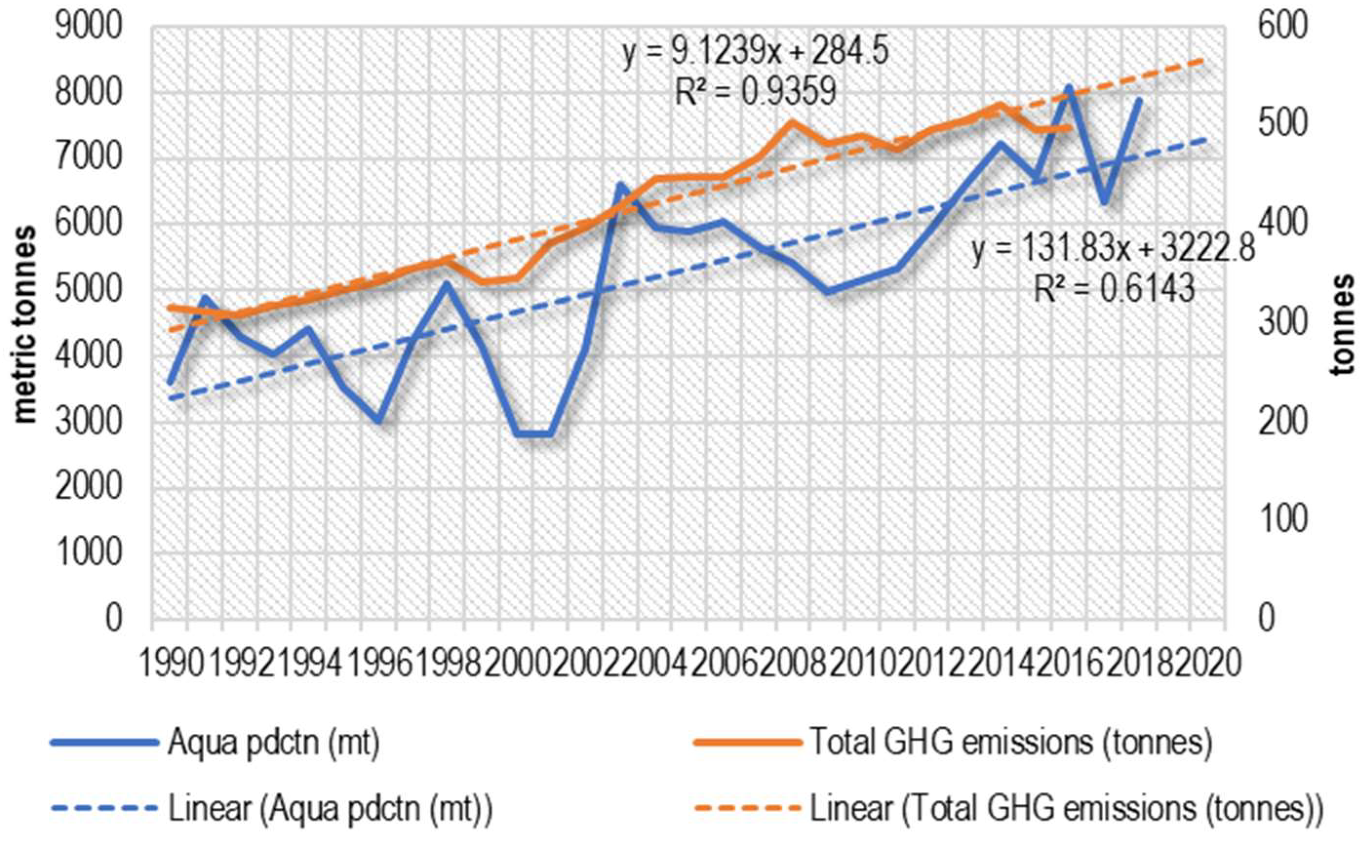
Figure 3 shows the increasing trend of aquaculture production and GHG emissions in South Africa. GHG emissions, on average, increased by 9.12 tonnes annually, while aquaculture production increased by 131.83 tonnes annually.

3.2. Empirical Results

Stationarity and order of integration were determined through a unit root test (

Table 2. Unit root test.

	Augmented Dickey Fuller (ADF) Test		Phillips–Perron (PP) Test
	I(0)	I(1)	I(0)	I(1)
In AQUAP	−3.049 **		−2.360	−5.240 ***
In GHG	−1.204	−4.504 ***	−1.204	−4.489 ***
In GDP	−1.451	−4.695 ***	−0.347	−5.380 ***
In BP	−1.262	−4.871 ***	−1.351	−4.871 ***

Note: Sig at *** 1%, ** 5%.

). The ARDL model was ideal because the variables were integrated into different orders. The Augmented Dickey–Fuller (ADF) shows that aquaculture production was stationary at levels, while greenhouse gas emissions, gross domestic product and beef production were stationary at first difference.

The ARDL Bounds test, as shown in

Table 3. ARDL Bounds test.

				In AQUAP	In GHG	In GDP	In BP
In AQUAP					0.070 *	−0.039	0.130
In AQUAPt−1				0.392 *	−0.059
In GHG				1.922 **		0.269 **	−0.967 *
In GHGt−1					0.638 ***		0.828
In GDP				−2.607	0.831 **		0.169
In GDPt−1				2.277	−0.734 **	0.953 ***
In BP				0.133	−0.123	0.015
In BPt−1					0.144 *	−0.080 *	0.717 ***
Constant				9.272 *	−2.077 *	1.087	−2.215
Model summary
Adjusted R-squared				0.442	0.854	0.994	0.784
Durbin–Watson statistic				1.411	2.099	1.338	2.090
F-statistic				4.959	21.955	771.954	19.120
Prob (F-statistic)				0.004	0.000	0.000	0.000
Bounds test
	Sig.	I(0)	I(1)
F-statistic	10%	2.72	3.77	3.663	1.206	4.469	2.422
	5%	3.23	4.35
	2.5%	3.69	4.89
	1%	4.29	5.61

Note: ***, ** and * indicate significance at 1%, 5%, and 10%, respectively.

, shows that there was long-run equilibrium cointegration in the gross domestic product model as the F-statistic in the bounds test was larger than the I(1) at the 5% level. The aquaculture production model was inconclusive as the F-statistic was between the I(0) and I(1), while there was no long-run equilibrium cointegration in the greenhouse gas emission and beef production models, respectively, as the F-statistics were below the I(0) at the 5% level. The ECM was, therefore, necessary to specify the long-run model in the GDP model, while the ARDL sufficed for the other models.

In the short run, $AQUA{P}_{t-1}$ and $GHG$ had a positive significant relationship with AQUAP at the 10% level (Table 3). Table 3 also shows that, in the short run, $AQUAP$, $GH{G}_{t-1}$, $GDP$ and $B{P}_{t-1}$ had a positive significant relationship with $GHG$ at the 10%, 1%, 5%, and 10% levels, respectively. $GD{P}_{t-1}$ had a negative significant relationship with $GHG$. $GHG$ and $GD{P}_{t-1}$ had a positive significant relationship with $GDP$ at the 5% and 1% levels, respectively, while $B{P}_{t-1}$ had a negative significant relationship at the 10% level. $GHG$ also had negative significant relationship with $BP$ at the 10% level, while $B{P}_{t-1}$ had a positive relationship at the 1% level.

In the long run, $GHG$ had a positive significant causal relationship with $GDP$ at the 5% level (

Table 4. Long-run relationship and error correction model regression for GDP model.

Dependent Variable
In GDP
Independent variable	Coefficient	Std. Error	t-Statistic	Prob
In AQUAP	−0.834	0.687	−1.215	0.239
In GHG	5.747	2.667	2.155	0.044
In BP	−1.379	1.399	−0.986	0.336
EC = In GDP-(5.747 In GHG − 0.834 In AQUAP − 1.379 In BP
ECM Regression
Variable	Coefficient	Std. Error	t-Statistic	Prob
D(In B)	0.015	0.040	0.391	0.700
CoinEq(−1) *	−0.047	0.010	−4.534	0.000
Constant	1.087	0.237	4.576	0.000
	Model summary
Adjusted R-squared	0.429
Durbin–Watson statistic	1.338
F-statistic	10.403
Prob (F-statistic)	0.000

). At a 1% increase $GHG$ increases $GDP$ by 5.75%. The error correction term shows that there was a long-run causal relationship in the model. The reversion to equilibrium was at an adjustment speed of 4.7%, and it will take 21.28 years $\left(\frac{1}{4.7\%}\right)$ to achieve equilibrium.

Table 5. Pairwise Granger causality test.

Null Hypothesis	F-Statistic
In GHG does not Granger cause In GDP	0.005
In GDP does not Granger cause In GHG	2.893
In AQUAP does not Granger cause In GDP	0.613
In GDP does not Granger cause In AQUAP	1.886
In BP does not Granger cause In GDP	8.660 ***
In GDP does not Granger cause In BP	4.359 **
In AQUAP does not Granger cause In GHG	2.537
In GHG does not Granger cause In AQUAP	4.248 *
In BP does not Granger cause In GHG	0.135
In GHG does not Granger cause In BP	6.151 **
In BP does not Granger cause In AQUAP	0.995
In AQUAP does not Granger cause In BP	3.598 *

Note: ***, ** and * indicate significance at 1%, 5% and 10%, respectively.

shows that there was bi-directional causality between $BP$ and $GDP$. The table also shows that GHG Granger caused $AQUAP$ and $BP$, while $AQUAP$ caused $BP$.

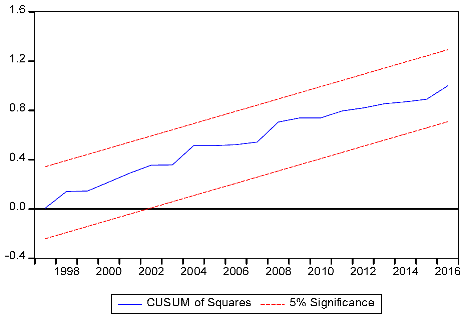
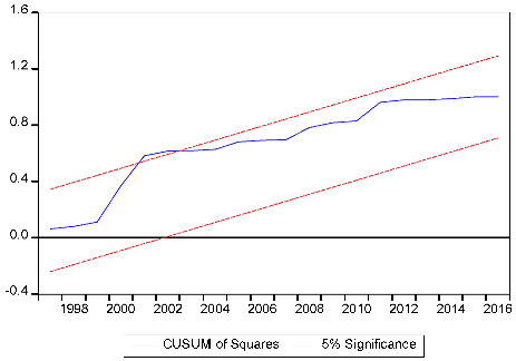
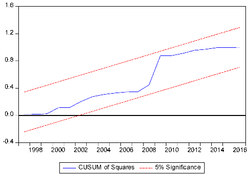
The diagnostic tests in

Table 6. Diagnostic tests.

	In AQUAP	In GHG	In GDP	In BP
Heteroscedasticity test
Breusch–Pagan Godfrey test	0.801 (0.562)	2.325 (0.081)	0.495 (0.776)	0.735 (0.646)
Multi-collinearity test
Breusch–Pagan Godfrey Serial Correlation LM test	4.202 (0.054)	0.133 (0.719)	2.297 (0.138)	0.117 (0.737)
Normality test
Jarque–Bera	0.223 (0.895)	0.680 (0.712)	0.662 (0.718)	1.989 (0.370)
Stability test
CUSUM of squares test
Sig values in parentheses

show that there was no heteroscedasticity in all models, as indicated by the Breusch–Pagan Godfrey tests which were all insignificant at the 5% level. This shows that there was no constant variance, and the models were homoscedastic. The Breusch–Pagan Godfrey Serial Correlation LM tests were also insignificant, indicating that the error terms were independent in all models and thus did not rely on the previous period’s value. The Jarque–Bera normality test shows that the error terms were normally distributed in all models. All the models were structurally stable, as shown by the CUSUM of squares test, and thus suitable for long-run decisions.

4. Discussion

The results show that aquaculture production ranged between 2819 tonnes and 8094 tonnes for the period between 1990 and 2020. Aquaculture production had an increasing trend, with an average annual increase of 131.83 tonnes. There was peak aquaculture output in 1991, 1998, 2003, and 2016. Low aquaculture production levels were observed in 1996, 2000–2001, 2009, and 2017. Adeleke et al. [3], DAFF [40], as well as Britz and Venter [41] concur that South African aquaculture has exhibited an increase, driven by a well-established high-value abalone subsector. A study by Mahlalela [42] found that, for the periods 1996, 2000, 2009, and 2017, increases corresponded to high rainfall anomalies in some parts of South Africa. Interestingly, these periods corresponded to periods of depressions in temperature [43]. Periods such as 1998, 2003, and 2016 had little to no rainfall and temperature anomalies [42,43] and were characterised by peak aquaculture output. In addition to climatic variables, a study by Britz [44] indicated that the growth in South Africa’s aquaculture sector is dependent on the extent and nature of public sector support. This is augmented through infrastructural capacity and institutional support for the growth of the sector. Furthermore, there exists a small but highly skilled manpower within public and private sectors, large endowments of research capacity in developing aquaculture technology and research funding facilities [44]. However, the sector has not been representative of the race/ethnic distribution or the lack of a comprehensive sector-level R&D strategy, awareness, and experience in aquaculture development.

GHG emissions averaged 412.23 tonnes, with peaks in 2004 and 2008 and a dip in 1999. A report by USAID [45] showed that between 1990 and 2014, GHG emissions in South Africa grew by 44%, with industrial processes contributing the largest change, followed by energy, land use change, forestry, and agriculture, respectively. A report by DEA [46] showed that between 1990 and 2000, GHG emissions had doubled for industrial processes and product use, increased for energy, and reduced for agriculture and waste. DEA [47] indicated that between 2000 and 2015, GHG emissions had increased by 23.1%, while Smith [48] noted that between 2000 and 2017, there was a 10.4% increase. The period between 2004 and 2008 corresponds to a peak in GDP growth in South Africa [49]. However, DEFFE [50] indicated that after 2009, GHG emissions stabilized and declined with an average annual decline of 1%. The increase in GHG emissions could be explained by the increase in electrification in South Africa since Eskom is the country’s biggest emitter [51]. The South African economy relies on a sustained coal-based energy supply, which leads to high GHG emissions. The period of 1999 also coincided with a depressed economic growth rate in the previous year.

The results showed a long-run relationship in the GDP model. In the long run, GHG emissions had a positive causal relationship with GDP. GHG emissions increased GDP by 7.75%. Reversion to equilibrium was at a speed of 4.7%, taking 21 to 28 years to achieve equilibrium. In the short run, GHG emissions and the previous period’s GDP had a significant positive relationship with GDP, while beef production had a negative relationship. Similar results were obtained from Khobai and Le Roux [52], who identified CO₂ emissions as having a causal relationship with economic growth in South Africa. Adebayo and Odugbesan [53] also found that there was positive interaction between economic growth and CO₂ emissions in South Africa. The study identified that energy use was the biggest emitter of GHG emissions. Adebayo and Odugbesan [53] explained this relationship through the Environmental Kuznets Curve (EKC), which was, however, not exhibited in the current study because, in the long run, GHG emissions had a positive relationship with GDP, whilst it was negative in the short run. This shows that South Africa is still in the developing stage of the EKC and is highly reliant on GHG-emitting energy to achieve economic growth in the long term. A sector-specific study in South Africa was conducted by Ngarava et al. [54] and highlighted that sector expansion did not necessarily lead to sustainable GHG emissions. Khobai and Le Roux [52] indicated that any GHG emission reduction strategy in South Africa would slow economic growth. According to Hughes and Herian [55], the growth of many economies was closely correlated with an increase in greenhouse gas emissions for the most prolonged time. Many economies use large quantities of energy in their production systems, releasing GHG. Similar findings were observed by Cederborg and Snöbohm [56], who stated that the growing per capita GDP motivates an increase in GHG emissions. Furthermore, increased GDP suggests high production levels, which contribute to the betterment of an economy [56].

In the short run, current aquaculture production had a significant positive relationship with the previous period’s aquaculture production and current GHG emissions. GHG emissions had a significant positive relationship with current aquaculture production, GDP, the previous period’s GHG emissions, and beef production, respectively. GHG emission Granger caused aquaculture production and beef production, while aquaculture production Granger caused beef production. According to Kurniawan et al. [57], environmental concerns, such as GHG emissions from aquaculture production, raise sustainability concerns. Aquaculture production tends to increase GHG emissions through fish faecal matter and feeding residues as well as protein-rich residual feed and excretory products. However, climate stressors induced by GHG emissions, such as ocean acidification, decrease in rainfall, increase in temperature, and increase in rainfall variability, have affected aquaculture production. This has been through reducing fish abundance, productivity and size as well as redistributing catch potential [58,59]. Ortega-Cisneros et al. [29] and van der Lingen [60] indicated that in South Africa, GHG emission-induced climate change could have varied environmental, ecological, and social effects on aquaculture production. Environmentally it increases ocean acidification, circulation patterns, extreme events, sea level rise as well as temperature increase. Ecologically, it can lead to the extinction of some fish species and changes in production and food availability, among other problems. Socially, poverty levels are increased, as well as changes in food security and increases in unemployment, amongst others. In South Africa, sea level temperature also increases, resulting in a shift of some marine species, community changes in resource structure, and competition which has economic bearing especially on value chain costs as well as the availability of aquaculture products, impacting livelihoods for aquaculture dependent communities [61,62,63]. The sector does, however, have a low GHG emission footprint [64], signifying how the wider circular economy has disproportionally affected aquaculture production.

The positive relationship between GHG emissions and beef production supports findings by Simdi and Seker [65]. According to Grossi et al. [66], the livestock sector requires significant natural resources and is responsible for close to a fifth of GHG emissions. About 45% of GHG emissions in livestock production are within feed production, while 39% is from enteric fermentation, 10% from manure storage, and 6% from processing and transportation. Furthermore, for enteric fermentation and manure storage in beef production, 91% of GHG emissions were from enteric fermentation, 6% from manure storage nitrous oxide, and 3% from manure storage methane [12,66]. Authors such as Rojas-Downing et al. [67] indicated that GHG emission-induced climate change tends to affect livestock production by impacting the quality of feed crop and forage, biodiversity, animal reproduction, livestock diseases, animal and meat production, as well as water availability, which tend to affect beef production.

The causality of aquaculture production and beef production can be explained by the complementarities of the food systems in terms of feed production. There is high dependence on manufactured feed and on meat and bone meal for aquaculture feed, whereupon livestock feed was also dependent upon fish meal [68,69].

In the short run, the current beef production had a significant positive relationship with the previous period’s beef production, while current GHG emissions had a significant negative relationship. The results further showed that beef production and GDP bi-directionally caused each other. Even though the agricultural sector in South Africa contributes less than 10% to the country’s GDP, livestock production constitutes between 42% and 46.7% of the agricultural GDP, with the country having 6% of the African continent’s cattle [70]. An increase in beef production will have an effect on the GDP, which will, in turn, increase disposable incomes, urbanisation and changes in tastes and preferences, and coupled with population growth, will induce growth in the livestock sector due to increased demand [71,72].

5. Conclusions

Aquaculture production in South Africa is still in its infancy; however, it carries a huge potential for food security and improved livelihoods as well as human and economic development. This is augmented by the good infrastructure, business institutions, supply chains, and supportive aquaculture legislation in place. However, this huge potential is offset by social and environmental concerns resulting from feed production, water pollution, and antimicrobial resistance. This is combined with factors such as climate change-induced extremes such as droughts, floods, global warming, ocean acidification, rainfall variation, salinity, and sea level rise, which are a result of GHG emissions. However, aquaculture production has also been responsible for GHG emissions through power utilisation, feed production, and logistics. The objective of the study was to ascertain the relationship between aquaculture production and GHG emissions in South Africa. The study used the autoregressive distributed lag—error correction model (ARDL-ECM) with time series data between 1990 and 2020.

The results showed that the mean aquaculture production in the period was 5200 tonnes annually and was explained by climatic variations such as temperature and rainfall anomalies. GHG gas emissions and GDP had peaks of 520 tonnes and US$673 trillion, respectively. Aquaculture production was increasing at an annual rate of 132 tonnes, while GHG emissions were increasing at 9.12 tonnes. The results in the GDP model exhibited a long-run relationship, with GHG emissions having a positive relationship with GDP. In the short run, GHG emissions had a positive relationship with GDP, while beef production had a negative relationship. Furthermore, there was bi-directional relationship between aquaculture production and GHG emissions in the short run. In addition, beef production and GDP had a bi-directional relationship in the short run. Beef production also had a positive relationship with aquaculture production in the short run. The study concludes that aquaculture production corresponds to climatic variations, which are induced by GHG emissions. However, GHG emissions did not have a long-run relationship with aquaculture production, but they did have one with GDP. In the short run, both aquaculture production and GHG emissions positively affect each other. In addition, aquaculture production and beef production function as complementarities, especially in feed production. The study recommends that aquaculture legislation in South Africa should consider GHG emissions which tend to affect and are affected by the sector. There is a need to promote sustainable production techniques in South Africa’s aquaculture industry, embracing renewable energy.

References

1. World Bank. Priorities for Sustainably Managing Sri Lanka’s Marine Fisheries, Coastal Aquaculture, and the Ecosystems That Support Them; World Bank: Washington, DC, USA, 2021. [Google Scholar]
2. FAO. Statistical Yearbook: World Food and Agriculture; Food and Agriculture Organization: Rome, Italy, 2021; ISBN 9789251343326. [Google Scholar]
3. Adeleke, B.; Robertson-andersson, D.; Moodley, G.; Adeleke, B.; Robertson-andersson, D.; Moodley, G. Aquaculture in Africa: A comparative review of Egypt, Nigeria and Uganda vis-a-vis South Africa. Rev. Fish. Sci. Aquac. 2021, 29, 167–197. [Google Scholar] [CrossRef]
4. PMG Commercial fishing organisations: Fish SA.; WWF & AquaCulture. 2020. Available online: https://pmg.org.za/committee-meeting/30478/ (accessed on 1 February 2022).
5. SADC-EU EPA South African Fisheries and the SADC-EU Economic Partnership Agreement. 2017. Available online: https://sadc-epa-outreach.com/images/files/sadc-eu-epa-fisheries-july-2017.pdf (accessed on 3 February 2022).
6. AgriSETA. Aquaculture Sub-Sector Skills Plan (2020–2021); AgriSETA: Arcadia, Pretoria, 2019; Available online: https://www.agriseta.co.za/wp-content/uploads/2021/02/Agriseta_Aquaculture_SSSP_DIGITAL.pdf (accessed on 7 December 2021).
7. WWF-SA. Fisheries: Facts and trends South Africa; WWF-SA: Cape Town, South Africa, 2011; Available online: http://awsassets.wwf.org.za/downloads/wwf_a4_fish_facts_report_lr.pdf (accessed on 8 August 2021).
8. World Bank Aquaculture Production (Metric Tons)-South Africa. 2021. Available online: https://data.worldbank.org/indicator/ER.FSH.AQUA.MT?locations=ZA (accessed on 17 March 2023).
9. DEFF. Operation Phakisa: Unlocking the Oceans Economy through Aquaculture; DEFF: Pretoria, South Africa, 2019. Available online: https://www.dffe.gov.za/sites/default/files/docs/publications/operation_phakisa_yearfive.pdf (accessed on 2 January 2022).
10. Fish SA. Fishing for a Sustainable and Equitable Future; Fish SA: Cape Town, South Africa, 2019. [Google Scholar]
11. Friedrich, E.; Trois, C. Current and future greenhouse gas (GHG) emissions from the management of municipal solid waste in the eThekwini Municipality—South Africa. J. Clean. Prod. 2016, 112, 4071–4083. [Google Scholar] [CrossRef]
12. Gerber, P.J.; Steinfeld, H.; Henderson, B.; Mottet, A.; Opio, C.; Dijkman, J.; Falcucci, A.; Tempio, G. Tackling climate change through livestock: A global assessment of emissions and mitigation opportunities. In Tackling Climate Change Through Livestock: A Global Assessment of Emissions and Mitigation Opportunities; Gerber, P.J., Steinfeld, H., Henderson, B., Mottet, A., Opio, C., Dijkman, J., Falcucci, A., Tempio, G., Eds.; Food and Agriculture Organization: Rome, Italy, 2013; Available online: http://www.fao.org/docrep/018/i3437e/i3437e00.htm (accessed on 3 October 2022).
13. Macleod, M.J.; Hasan, M.R.; Robb, D.H.F. Quantifying greenhouse gas emissions from global aquaculture. Sci. Rep. 2020, 10, 11679. [Google Scholar] [CrossRef] [PubMed]
14. Ahmed, N.; Thompson, S.; Glaser, M. Global aquaculture productivity, environmental sustainability, and climate change adaptability. Environ. Manage. 2019, 63, 159–172. [Google Scholar] [CrossRef] [PubMed]
15. Raul, C.; Pattanaik, S.S.; Prakash, S.; Sreedharan, K.; Bharti, S. Greenhouse Gas Emissions from Aquaculture Systems. World Aquac. 2020, 57, 57–61. [Google Scholar]
16. Subasinghe, R.P.; Delamare-Deboutteville, J.; Mohan, C.V.; Phillips, M.J. Vulnerabilities in aquatic animal production. Rev. Sci. Tech. 2019, 38, 423–436. [Google Scholar] [CrossRef] [PubMed]
17. Barange, M.; Cochrane, K.L. Impacts of climate change on fisheries and aquaculture: Conclusions. In Impacts of Climate Change on Fisheries and Aquaculture: Synthesis of Current Knowledge, Adaptation and Mitigation Options; Barange, M., Bahri, T., Beveridge, M.C.M., Cochrane, K.L., Funge-Smith, S., Poulain, F., Eds.; Food and Agriculture Organization: Rome, Italy, 2018; ISBN 978-92-5-130607-9. [Google Scholar]
18. Adhikari, S.; Cahudhari, A.; Barlaya, G.; Rathod, R.; Mandal, R.N.; Ikmail, S.; Saha, G.S.; De, H.; Iyemperumal, S.; Mahapatra, A.S.; et al. Adaptation and Mitigation Strategies of Climate Change Impact in Freshwater Aquaculture in some states of India. J. Fish. 2018, 12, 16–21. [Google Scholar] [CrossRef]
19. Barange, M.; Bahri, T.; Beveridge, M.C.M.; Cochrane, K.L.; Funge-Smith, S.; Poulain, F. (Eds.) Impacts of Climate Change on Fisheries and Aquaculture; Food and Agriculture Organization: Rome, Italy, 2018; ISBN 9789251306079. [Google Scholar]
20. Liddle, B. Environmental Modelling & Software Population, affluence, and environmental impact across development: Evidence from panel cointegration modeling q. Environ. Model. Softw. 2013, 40, 255–266. [Google Scholar] [CrossRef]
21. Robb, D.H.F.; Macleod, M.J.; Hasan, M.R.; Soto, D. Greenhouse Gas Emissions from Aquaculture: A Lifecycle Assessment of Three Asian Systems; FAO: Rome, Italy, 2017. [Google Scholar]
22. Hammer, A.J.; Millar, C.; Hennige, S.J. Reducing carbon emissions in aquaculture: Using Carbon Disclosures to identify unbalanced mitigation strategies. Environ. Impact Assess. Rev. 2022, 96, 106816. [Google Scholar] [CrossRef]
23. Xu, C.; Su, G.; Zhao, K.; Xu, X.; Li, Z.; Hu, Q.; Xue, Y.; Xu, J. Current status of greenhouse gas emissions from aquaculture in China. Water Biol. Secur. 2022, 1, 100041. [Google Scholar] [CrossRef]
24. Kosten, S.; Almeida, R.M.; Barbosa, I.; Mendonça, R.; Santos Muzitano, I.; Sobreira Oliveira-Junior, E.; Vroom, R.J.E.; Wang, H.J.; Barros, N. Better assessments of greenhouse gas emissions from global fish ponds needed to adequately evaluate aquaculture footprint. Sci. Total Environ. 2020, 748, 141247. [Google Scholar] [CrossRef]
25. Rasenberg, M.; Poelman, M.; Smith, S.; Hoof, L. Van GHG Emissions in Aquatic Production Systems and Marine Fisheries; IMARES: Wageningen, the Netherlands, 2013. [Google Scholar]
26. de Sousa-Neto, E.R.; Gomes, L.; Nascimento, N.; Pacheco, F.; Ometto, J.P. Land Use and Land Cover Transition in Brazil and Their Effects on Greenhouse Gas Emissions; Academic Press: Cambridge, MA, USA, 2018; pp. 309–321. [Google Scholar] [CrossRef]
27. DAFF. Integrated Growth and Development Plan; DAFF: Pretoria, South Africa, 2012. [Google Scholar]
28. Mujuru, M.; Dube, T.; Mabizela, H.; Ntuli, N. Evaluating greenhouse gas emission reductions by using solar water heaters: A case of low income households in Ekurhuleni, South Africa. Phys. Chem. Earth Parts A/B/C 2020, 116, 102843. [Google Scholar] [CrossRef]
29. Ortega-cisneros, K.; Cochrane, K.L.; Rivers, N.; Sauer, W.H.H.; Rice, J.; Ortega-cisneros, K. Assessing South Africa’s potential to address climate change impacts and adaptation in the fisheries sector. Front. Mar. Sci. 2021, 8, 652955. [Google Scholar] [CrossRef]
30. Jiang, Q.; Bhattarai, N.; Pahlow, M.; Xu, Z. Environmental sustainability and footprints of global aquaculture. Resour. Conserv. Recycl. 2022, 180, 106183. [Google Scholar] [CrossRef]
31. Mayers, J.; Batchelor, C.; Bond, I.; Hope, R.; Morrison, E.; Wheeler, B. Water Ecosystem Services and Poverty under Climate Change: Key Issues and Research Priorities; Natural Resources Issues No. 17; International Institute for Environment and Development (UK): London, UK, 2009; ISBN 9781843696872. Available online: http://pubs.iied.org/13549IIED.html (accessed on 2 December 2021).
32. Ngarava, S. Relationship between economic diversification and CO2 emissions: ARDL-EC modeling in South Africa ARDL-EC modeling in South Africa. Dev. Stud. Res. 2021, 8, 264–279. [Google Scholar] [CrossRef]
33. Coulibaly, G.R.; Akia, S.A. Export structure and economic growth in a developing country: Case of Cote d’Ivoire. Munich Pers. RePEc Arch. 2017. Available online: https://mpra.ub.uni-muenchen.de/id/eprint/91374 (accessed on 2 March 2023).
34. Kohler, M. CO2 emissions, energy consumption, income and foreign trade: A South African perspective. Energy Policy 2013, 63, 1042–1050. [Google Scholar] [CrossRef]
35. Adeleye, N. Autoregressive Distributed Lag (ARDL): Specification. 2018. Available online: http://cruncheconometrix.org.ng (accessed on 8 July 2021).
36. Ritchie, H.; Roser, M.; CO2 and greenhouse gas emissions. Our World Data. 2020. Available online: https://ourworldindata.org/co2-and-other-greenhouse-gas-emissions (accessed on 8 January 2021).
37. World Bank World Development Indicators: Aquaculture Production (Metric Tonnes). 2022. Available online: https://databank.worldbank.org/source/world-development-indicators# (accessed on 8 January 2021).
38. Quantec Easydata Production and Consumption of Beef and Veal: Total Production. Available online: https://www.easydata.co.za/dataset/AGR/timeseries/AGR-T060S001/ (accessed on 8 January 2021).
39. Odhiambo, N.M. Economic growth and carbon emissions in South Africa: An empirical investigation. J. Appl. Bus. Res. 2012, 28, 75–84. [Google Scholar]
40. DAFF. Aquaculture yearbook 2016 South Africa, Pretoria, South Africa. 2016. Available online: https://www.nda.agric.za/doaDev/sideMenu/fisheries/03_areasofwork/Aquaculture/AquaDocumentation/DAFF %0AYearbook 2016.5Mb.pdf (accessed on 3 October 2022).
41. Britz, P.J.; Venter, S. Aquaculture review: South Africa. World Aquac. 2016, 47, 19–28. [Google Scholar]
42. Mahlalela, P.T.; Blamey, R.C.; Hart, N.C.G.; Reason, C.J.C. Drought in the Eastern Cape region of South Africa and trends in rainfall characteristics. Clim. Dyn. 2020, 55, 2743–2759. [Google Scholar] [CrossRef]
43. World Bank. Climate Change Knowledge Portal: South Africa. 2022. Available online: https://climateknowledgeportal.worldbank.org/country/south-africa/climate-data-historical#:~:text=South Africa is highly vulnerable,fed agriculture and natural resources.&text=Mean annual temperature for South,C(June%2C July) (accessed on 15 February 2022).
44. Britz, P.J. A study on the status of aquaculture production and trade in South Africa. Enviro-Fish Africa 2007, 2, 24.
45. USAID. Greenhouse Gas Emissions in South Africa; USAID: Washington, DC, USA, 2014. [Google Scholar]
46. DEA. Greenhouse Gas Inventory for South Africa: 1990–2000; DEA: Pretoria, South Africa, 2009; Available online: https://static.pmg.org.za/docs/090812greenhouseinventory.pdf (accessed on 18 July 2021).
47. DEA. GHG National Inventory Report: South Africa (2000–2015); DEA: Pretoria, South Africa, 2015; Available online: https://unfccc.int/sites/default/files/resource/South Africa NIR 2017.pdf (accessed on 7 April 2021).
48. Smith T South Africa’s Greenhouse Gas Emissions on the Rise, Says Report. 2021. Available online: https://www.esi-africa.com/industry-sectors/finance-and-policy/south-africas-greenhouse-gas-emissions-on-the-rise-says-report/#:~:text=Greenhouse gas emissions in South,10.4%25 between 2000 and 2017.&text=There was an annual average,Environment on Tuesday (accessed on 19 February 2022).
49. World Bank. GDP (current US$)—Sub Saharan Africa. 2022. Available online: https://data.worldbank.org/indicator/NY.GDP.MKTP.CD?locations=ZG (accessed on 20 January 2022).
50. DEFFE. National GHG Inventory Report South Africa; DEFFE: Pretoria, South Africa, 2017. [Google Scholar]
51. Africa Check South Africa the 12th Biggest Source of Greenhouse Gases? Yes, but That’s Not the Only Measure that Matters. 2021. Available online: https://www.polity.org.za/article/south-africa-the-12th-biggest-source-of-greenhouse-gases-yes-but-thats-not-the-only-measure-that-matters-2021-04-19#:~:text=Yes%2C but that’s not the only measure that matters,-19th April 2021&text=“South Africa is the wo (accessed on 17 February 2022).
52. Khobai, H.; Roux, P. Le The Relationship between Energy Consumption, Economic Growth and Carbon Dioxide Emission: The Case of South Africa. Int. J. Energy Econ. Policy 2017, 7, 102–109. [Google Scholar]
53. Adebayo, T.S.; Odugbesan, J.A. Modeling CO2 emissions in South Africa: Empirical evidence from ARDL based bounds and wavelet coherence techniques. Environ. Sci. Pollut. Res. 2021, 28, 9377–9389. [Google Scholar] [CrossRef] [PubMed]
54. Ngarava, S.; Zhou, L.; Ayuk, J.; Tatsvarei, S. Achieving food security in a climate change environment: Considerations for Environmental Kuznets Curve use in the South African agricultural sector. Climate 2019, 7, 108. [Google Scholar] [CrossRef] [Green Version]
55. Hughes, L.; Herian, A. The Correlation between GDP and Greenhouse Gas Emissions. 2017. Available online: https://policyoptions.irpp.org/magazines/september-2017/the-correlation-between-gdp-and-greenhouse-gas-emissions/ (accessed on 19 February 2022).
56. Cederborg, A.J.; Snöbohm, S. Is There a Relationship between Economic Growth and Carbon Dioxide Emissions? 2016. Available online: https://www.diva-portal.org/smash/get/diva2:1076315/FULLTEXT01.pdf (accessed on 19 February 2022).
57. Kurniawan, S.B.; Ahmad, A.; Rahim, N.F.M.; Said, N.S.M.; Alnawajha, M.M.; Imron, M.F.; Abdullah, S.R.S.; Othman, A.R.; Ismail, N.‘I.; Hasan, H.A. Aquaculture in Malaysia: Water-related environmental challenges and opportunities for cleaner production. Environ. Technol. Innov. 2021, 24, 101913. [Google Scholar] [CrossRef]
58. Bjørndal, T.; Tusvik, A. Economic Analysis of the Contrinutions of Capture Fisheries and Aquaculture to Future Food Security; Centre for Applied Research at NHH: Bergen, Norway, 2020. [Google Scholar]
59. Tran, N.; Shikuku, K.M.; Peart, J.; Chan, C.Y.; Chu, L.; Bailey, C.; Valdivia, R. A review of economic analysis of climate change impacts and adaptation in fisheries and aquaculture. SocArXiv Pap. 2021, 1–45. [Google Scholar] [CrossRef]
60. van der Lingen, C.D. Adapting to climate change in the South African small pelagic fishery. In Adaptive Management of Fisheries in Response to Climate Change; Bahri, T., Vasconcellos, M., Welch, D., Johnson, J., Perry, I.R., Ma, X., Sharma, R., Eds.; Technical Paper No. 667; FAO Fisheries and Aquaculture: Rome, Italy, 2021; pp. 177–194. [Google Scholar]
61. Cochrane, K.L.; Eggers, J.; Sauer, W.H.H. A diagnosis of the status and effectiveness of marine fisheries management in South Africa based on two representative case studies. Mar. Policy 2020, 112, 103774. [Google Scholar] [CrossRef]
62. Cochrane, K.L.; Ortega-Cisneros, K.; Iitembu, J.A.; dos Santos, C.I.; Sauer, W.H.H. Application of a general methodology to understand vulnerability and adaptability of the fisheries for small pelagic species in the Benguela countries: Angola, Namibia and South Africa. Afr. J. Mar. Sci. 2020, 42, 473–493. [Google Scholar] [CrossRef]
63. Bolton, J.J.; Anderson, R.J.; Smit, A.J.; Rothman, M.D. South African kelp moving eastwards: The discovery of Ecklonia Maxima (Osbeck) Papenfuss at De Hoop Nature Reserve on the South Coast of South Africa. Afr. J. Mar. Sci. 2012, 34, 147–151. [Google Scholar] [CrossRef]
64. Barends-jones, V. Carbon Footprint Report: Departmental Research Farms (2019–2020); Western Cape Department of Agriculture Division for Macro & Resource Economics: Cape Town, South Africa, 2021; Available online: https://www.elsenburg.com/wp-content/uploads/2022/02/2021-Carbon-Footprint-Research-Farms-2019-20.pdf (accessed on 19 March 2023).
65. Simdi, H.; Seker, A. A change is gonna come: Will traditional meat production end ? Environ. Sci. Pollut. Res. 2021, 29, 30470–30485. [Google Scholar] [CrossRef] [PubMed]
66. Grossi, G.; Goglio, P.; Vitali, A.; Williams, A.G. Livestock and climate change: Impact of livestock on climate and mitigation strategies. Anim. Front. 2019, 9, 69–76. [Google Scholar] [CrossRef] [PubMed] [Green Version]
67. Rojas-downing, M.M.; Nejadhashemi, A.P.; Harrigan, T.; Woznicki, S.A. Climate change and livestock: Impacts, adaptation and mitigation. Clim. Risk Manag. 2017, 16, 145–163. [Google Scholar] [CrossRef]
68. MacLeod, M.; Hasan, M.; Robb, D.H.F.; Mamun-Ur-Rashid, M. Quantifying and Mitigating Greenhouse Gas Emissions from Global Aquaculture Quantifying and Mitigating; Technical Paper No. 626; FAO Fisheries and Aquaculture: Rome, Italy, 2019. [Google Scholar]
69. Kristofersson, D.; Anderson, J.L. Is there a relationship between fisheries and farming? Interdependence of fisheries, animal production and aquaculture. Mar. Policy 2006, 30, 721–725. [Google Scholar] [CrossRef]
70. Ngarava, S. Evaluating Livestock Development Programmes through the Production Risk Interface: Case of the Kaonafatso ya Dikgomo (KyD) Scheme in South Africa. Doctoral Thesis, University of Fort Hare, Alice, South Africa, 2019. [Google Scholar]
71. Meissner, H.H.; Scholtz, M.M.; Palmer, A.R. Sustainability of the South African livestock sector towards 2050 Part 1: Worth and impact of the sector. S. Afr. J. Anim. Sci. 2013, 43, 282–297. [Google Scholar] [CrossRef]
72. Meissner, H.H.; Scholtz, M.M.; Engelbrecht, F.A. Sustainability of the South African livestock sector towards 2050 part 2: Challenges, changes and required implementations. S. Afr. J. Anim. Sci. 2013, 43, 289–319. [Google Scholar] [CrossRef] [Green Version]
Figure 1. Aquaculture production in South Africa (1974–2020). Source: FAO [2] and World Bank [8].
Water 15 01253 g001
Figure 2. Conceptual framework. Source: [31].
Water 15 01253 g002
Figure 3. Aquaculture production and greenhouse gas emissions in South Africa (1990–2020).
Water 15 01253 g003