
Estimating the Specific Yield and Groundwater Level of an Unconfined Aquifer Using Time-Lapse Electrical Resistivity Imaging in the Pingtung Plain, Taiwan

 ,
, 
 ,
, 
Abstract
1. Introduction
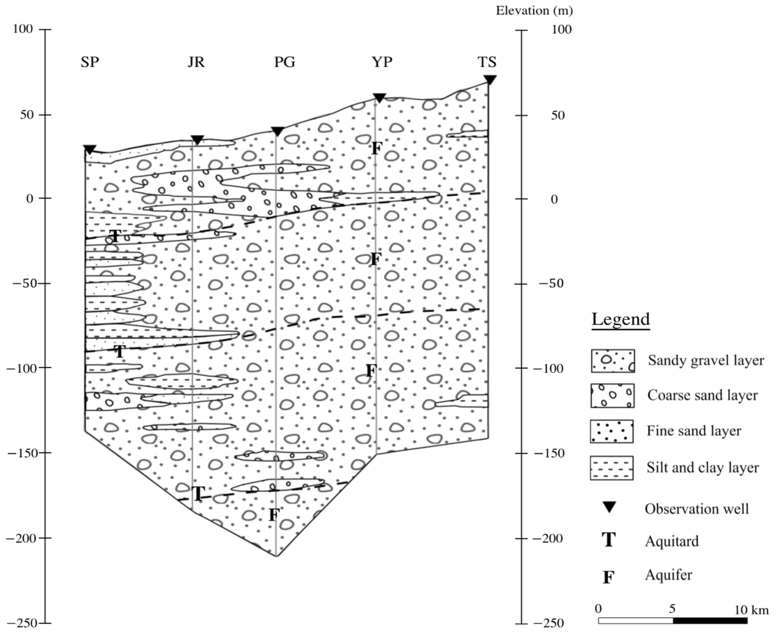
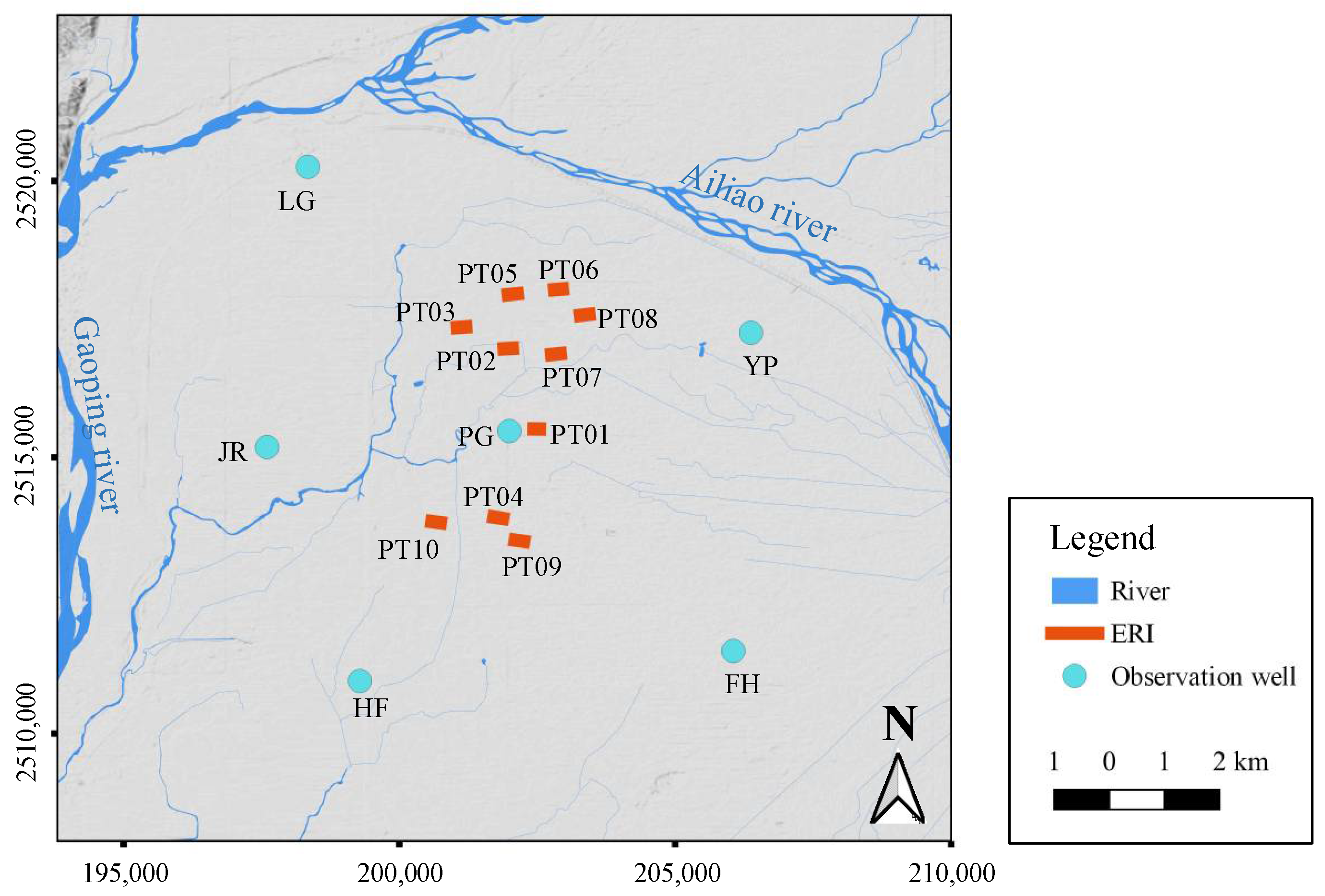
2. Study Area
3. Materials and Methods
3.1. Electrical Resistivity Imaging Data Acquisition and Processing
3.2. Empirical Estimation of Hydraulic Parameter from Resistivity Data
4. Results
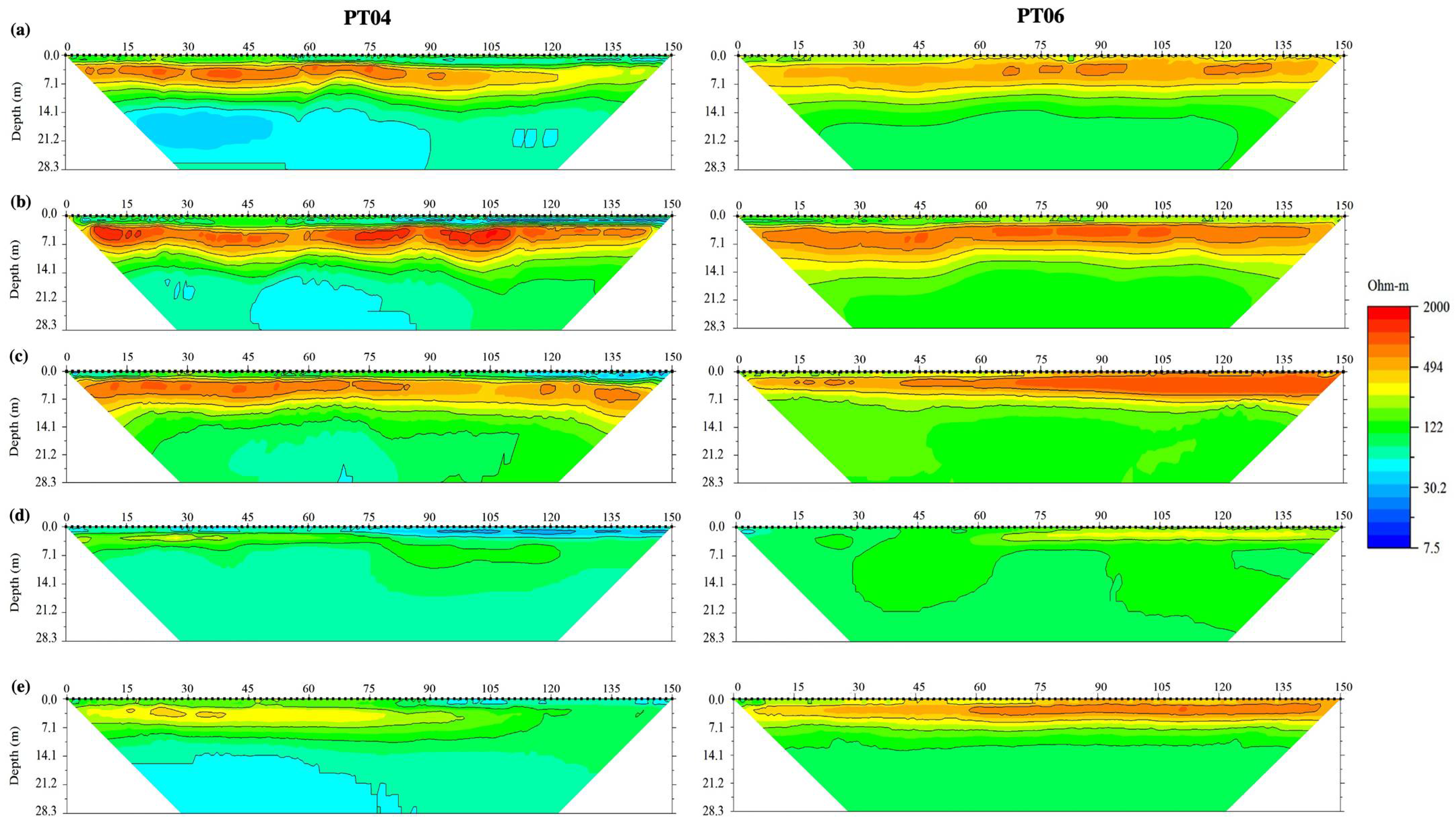
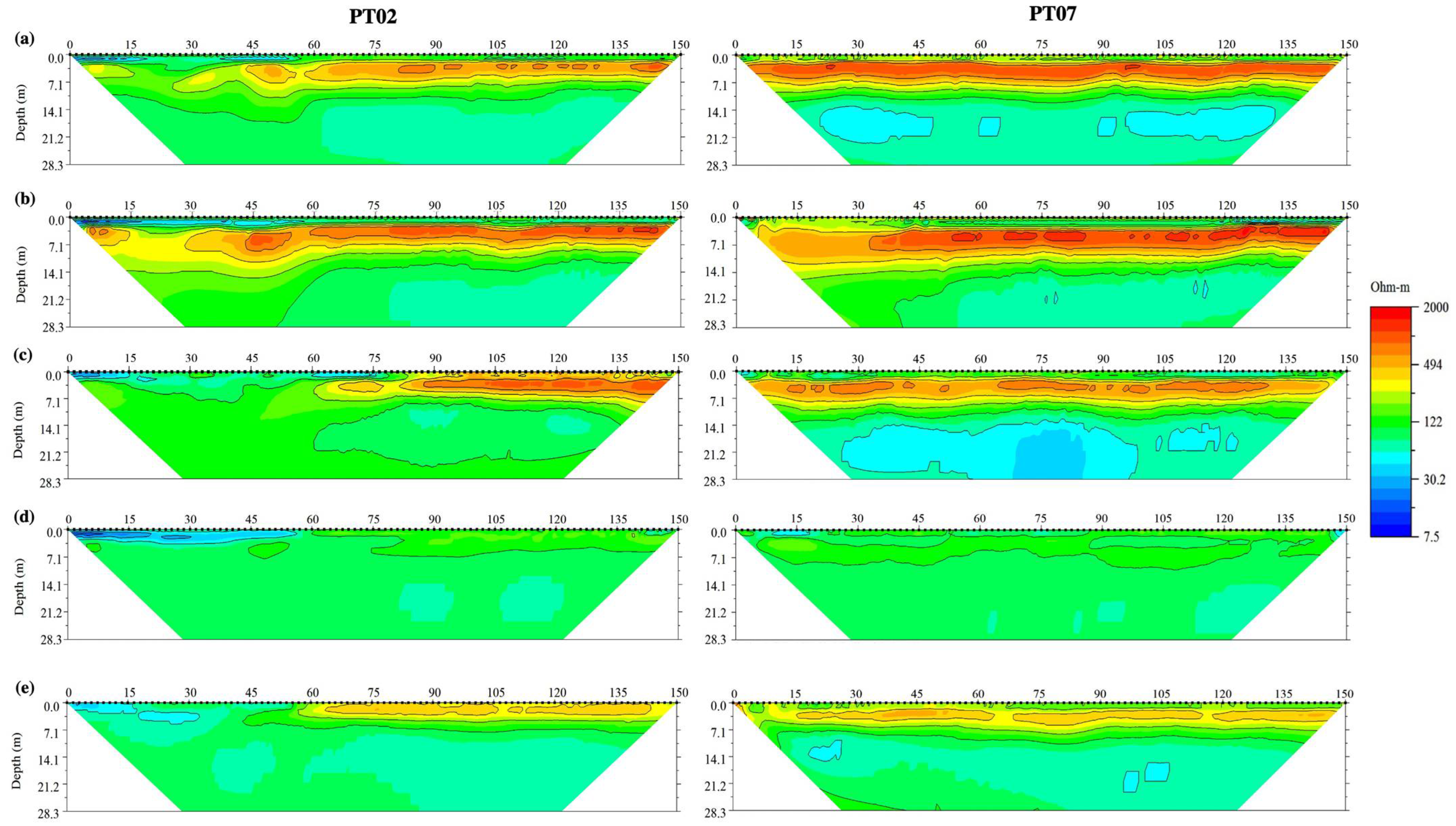
4.1. Time-Lapse ERI Survey
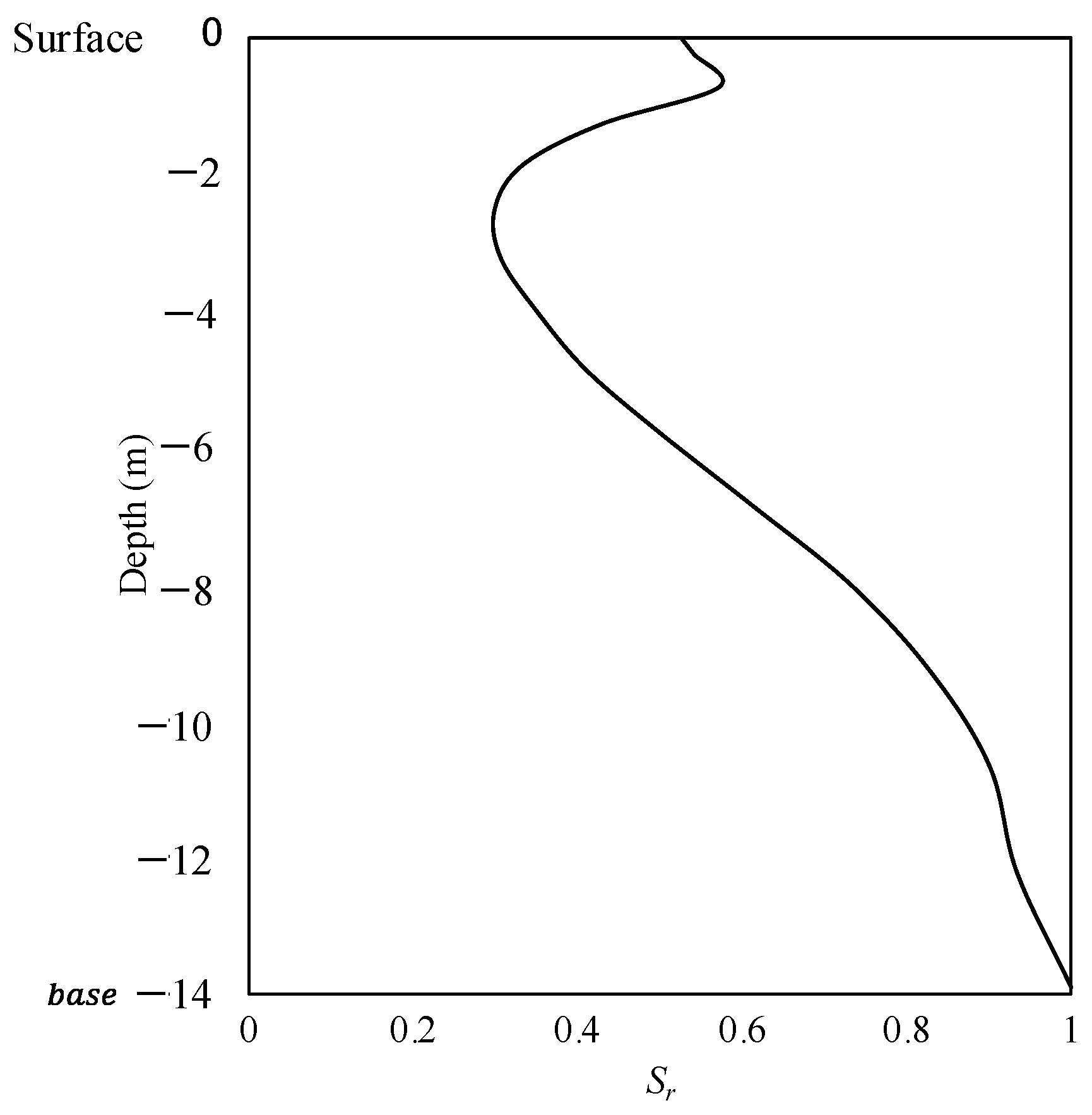
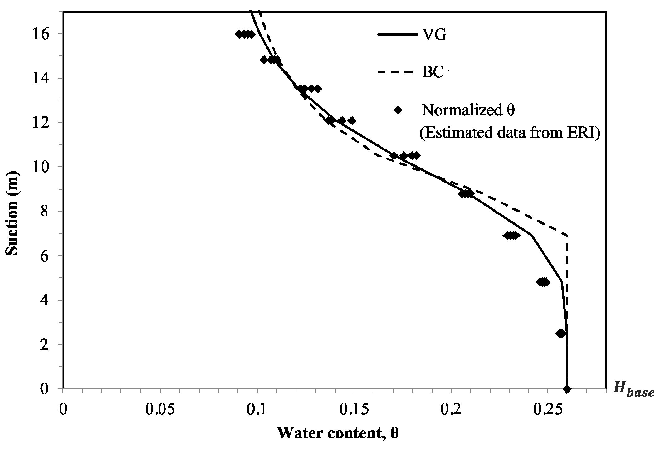
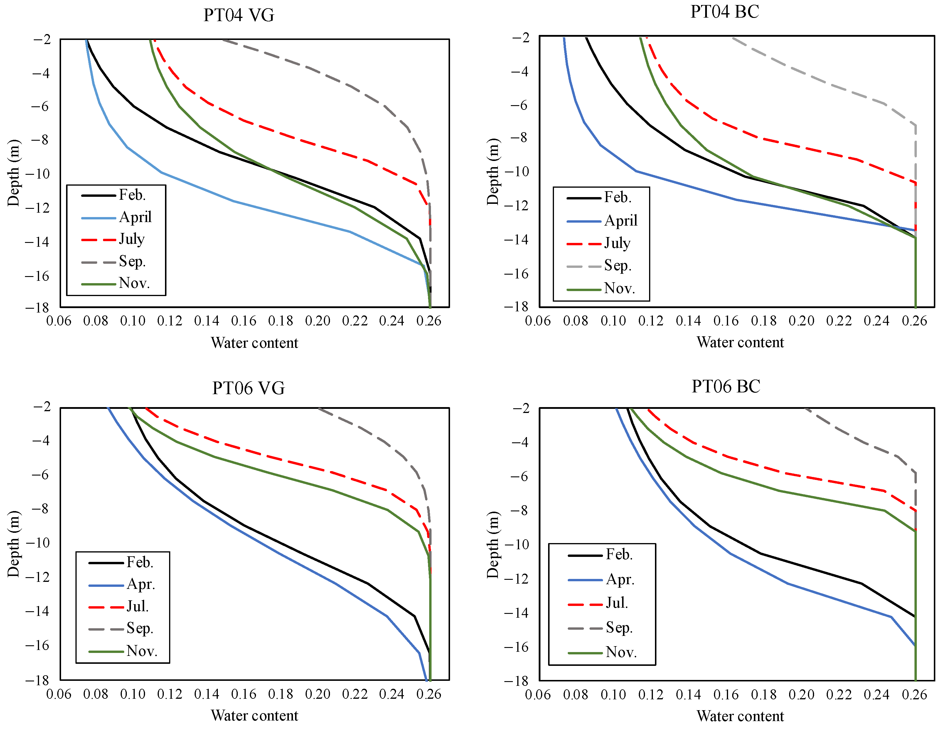
4.2. Soil–Water Characteristic Curve (SWCC) and Groundwater Level (GWL)
4.3. Theoretical Specific Yield
5. Discussion
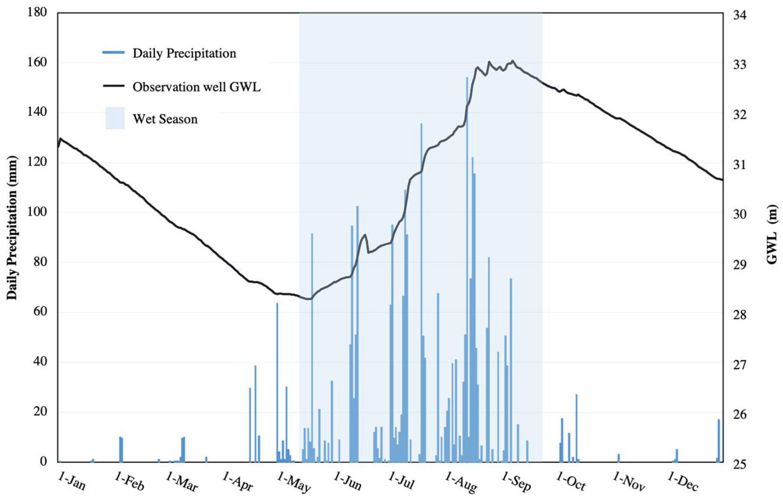
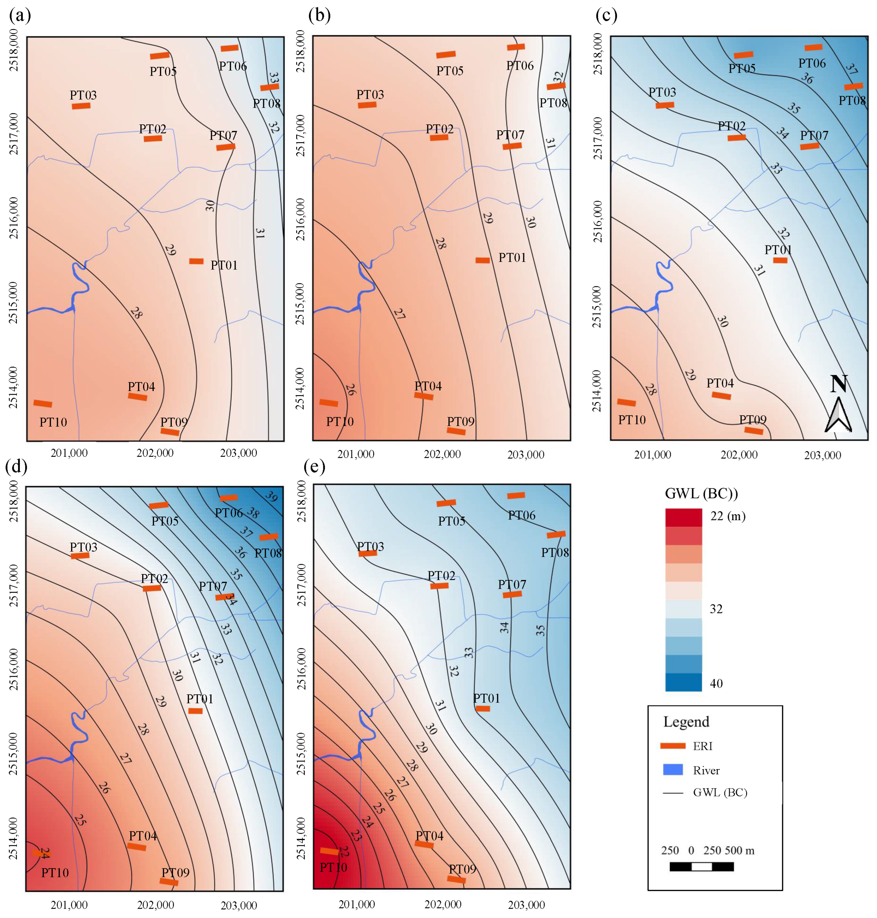
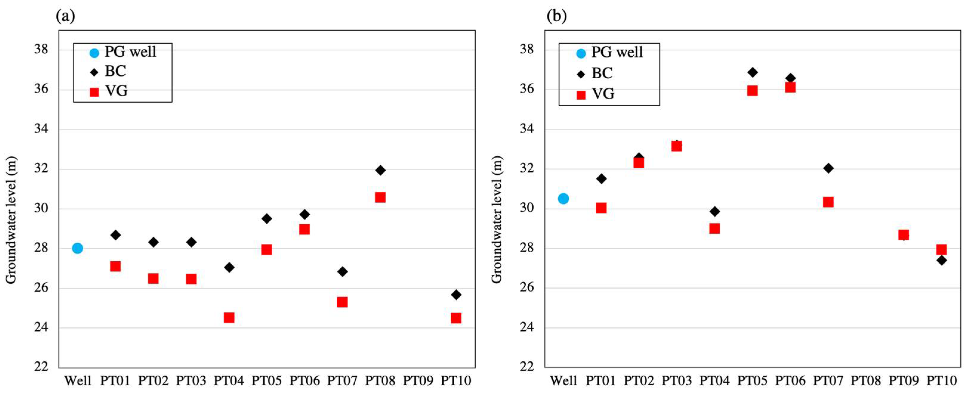
5.1. Groundwater Level Difference for Wet and Dry Seasons
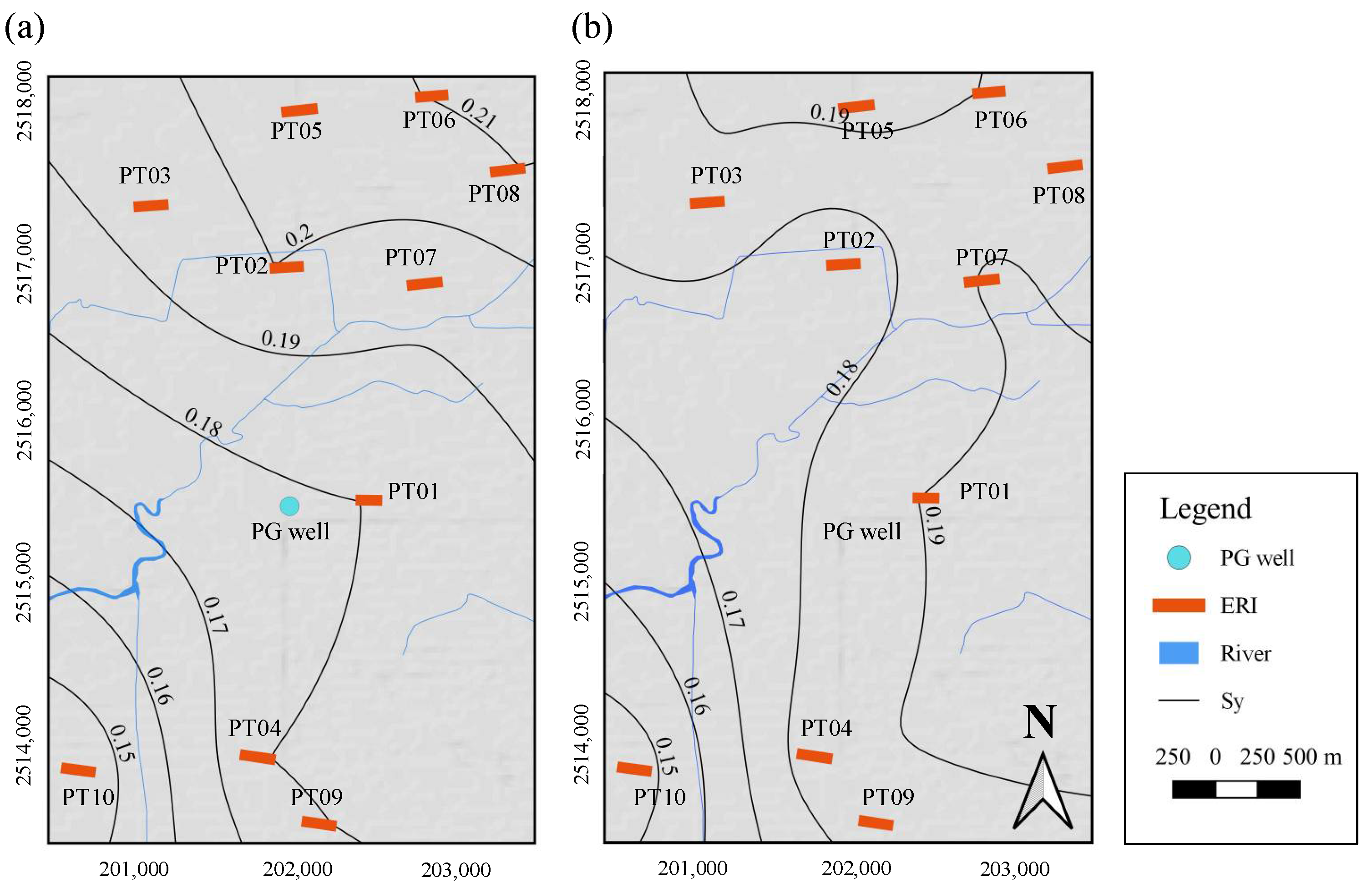
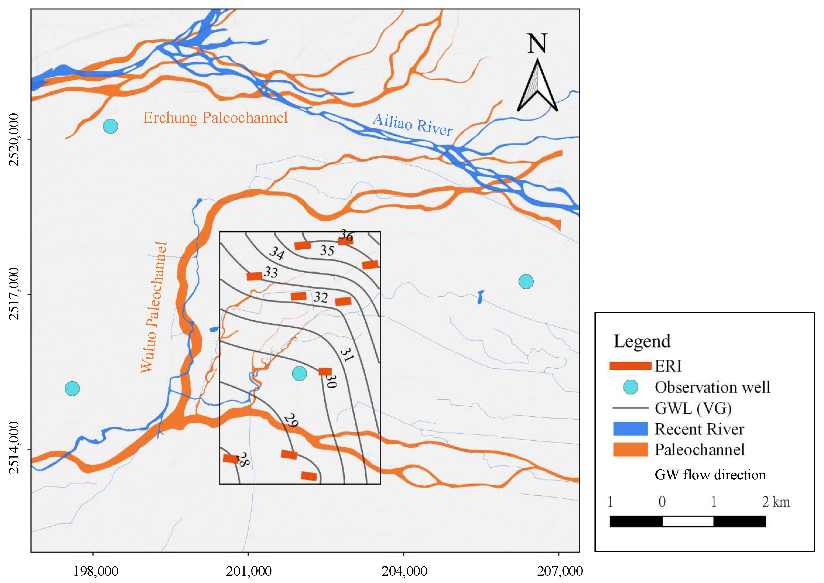
5.2. Groundwater Distribution and Paleochannel
5.3. SWCC Efficiency in Determining Hydraulic Parameters
6. Conclusions
Author Contributions
Funding
Data Availability Statement
Conflicts of Interest
References
- Gehman, C.L.; Harry, D.L.; Sanford, W.E.; Stednick, J.D.; Beckman, N.A. Estimating specific yield and storage change in an unconfined aquifer using temporal gravity surveys. Water Resour. Res. 2009, 45. [Google Scholar] [CrossRef]
- Vouillamoz, J.-M.; Lawson, F.; Yalo, N.; Descloitres, M. The use of magnetic resonance sounding for quantifying specific yield and transmissivity in hard rock aquifers: The example of Benin. J. Appl. Geophys. 2014, 107, 16–24. [Google Scholar] [CrossRef]
- Chen, X.; Goeke, J.; Ayers, J.F.; Summerside, S. Observation Well Network Design for Pumping Test in Unconfined Aquifer. J. Am. Water Resour. Assoc. 2003, 39, 17–32. [Google Scholar] [CrossRef]
- Archie, G.E. The Electrical Resistivity Log as an Aid in Determining Some Reservoir Characteristics. Trans. AIME 1942, 146, 54–62. [Google Scholar] [CrossRef]
- Di Maio, R.; Piegari, E.; Todero, G.; Fabbrocino, S. A combined use of Archie and van Genuchten models for predicting hydraulic conductivity of unsaturated pyroclastic soils. J. Appl. Geophy. 2015, 112, 249–255. [Google Scholar] [CrossRef]
- Lu, D.; Huang, D.; Xu, C. Estimation of hydraulic conductivity by using pumping test data and electrical resistivity data in faults zone. Ecol. Indic. 2021, 129, 107861. [Google Scholar] [CrossRef]
- Niwas, S.; Celik, M. Equation estimation of porosity and hydraulic conductivity of Ruhrtal aquifer in Germany using near surface geophysics. J. Appl. Geophys. 2012, 84, 77–85. [Google Scholar] [CrossRef]
- Van Genuchten, M.T. A closed-form equation for predicting the hydraulic conductivity of unsaturated soils. Soil Sci. Soc. Am. J. 1980, 44, 892–898. [Google Scholar] [CrossRef]
- Brooks, R.H. Hydraulic Properties of Porous Media; Colorado State University: Fort Collins, CO, USA, 1965. [Google Scholar] [CrossRef]
- Tijani, M.N.; Obini, N.; Inim, I.J. Estimation of aquifer hydraulic parameters and protective capacity in basement aquifer of south-western Nigeria using geophysical techniques. Environ. Earth Sci. 2021, 80, 466. [Google Scholar] [CrossRef]
- de Almeida, A.; Maciel, D.F.; Sousa, K.F.; Nascimento, C.T.C.; Koide, S. Vertical electrical sounding (VES) for estimation of hydraulic parameters in the porous aquifer. Water 2021, 13, 170. [Google Scholar] [CrossRef]
- Vogelgesang, J.A.; Holt, N.; Schilling, K.E.; Gannon, M.; Tassier-Surine, S. Using high-resolution electrical resistivity to estimate hydraulic conductivity and improve characterization of alluvial aquifers. J. Hydrol. 2020, 580, 123992. [Google Scholar] [CrossRef]
- Boucher, M.; Favreau, G.; Vouillamoz, J.-M.; Nazoumou, Y.; Legchenko, A. Estimating specific yield and transmissivity with magnetic resonance sounding in an unconfined sandstone aquifer (Niger). Hydrogeol. J. 2009, 17, 1805–1815. [Google Scholar] [CrossRef]
- Blainey, J.B.; Ferré, T.P.; Cordova, J.T. Assessing the likely value of gravity and drawdown measurements to constrain estimates of hydraulic conductivity and specific yield during unconfined aquifer testing. Water Resour. Res. 2007, 43. [Google Scholar] [CrossRef]
- Tizro, A.T.; Voudouris, K.; Basami, Y. Estimation of porosity and specific yield by application of geoelectrical method–a case study in western Iran. J. Hydrol. 2012, 454, 160–172. [Google Scholar] [CrossRef]
- Frohlich, R.K.; Parke, C.D. The electrical resistivity of the vadose zone—Field survey. Groundwater 1989, 27, 524–530. [Google Scholar] [CrossRef]
- Farzamian, M.; Monteiro Santos, F.A.; Khalil, M.A. Estimation of unsaturated hydraulic parameters in sandstone using electrical resistivity tomography under a water injection test. J. Appl. Geophys. 2015, 121, 71–83. [Google Scholar] [CrossRef]
- Kaleris, V.K.; Ziogas, A.I. Using electrical resistivity logs and short duration pumping tests to estimate hydraulic conductivity profiles. J. Hydrol. 2020, 590, 125277. [Google Scholar] [CrossRef]
- Chang, P.-Y.; Chang, L.-C.; Hsu, S.-Y.; Tsai, J.-P.; Chen, W.-F. Estimating the hydrogeological parameters of an unconfined aquifer with the time-lapse resistivity-imaging method during pumping tests: Case studies at the Pengtsuo and Dajou sites, Taiwan. J. Appl. Geophys. 2017, 144, 134–143. [Google Scholar] [CrossRef]
- Dahlin, T.; Zhou, B. A numerical comparison of 2D resistivity imaging with 10 electrode arrays. Geophys. Prospect. 2004, 52, 379–398. [Google Scholar] [CrossRef]
- Chen, W.-S.; Yang, C.-C.; Yang, H.-C.; Yu, N.-T.; Chen, Y.-C.; Wu, L.-C.; Lin, C.-W.; Chang, H.-C.; Shih, R.-C.; Lin, W.-H. Geomorphic Characteristics of the mountain-valley in the subsidence enviroment of the Taipei basin, Lanyang plain and Pingtung plain. Bull. Cent. Geol. Surv. 2004, 17, 79–106. [Google Scholar]
- Survey, C.G. Project of Groundwater Monitoring Network in Taiwan during First Stage-Research Report of Pingtung Plain, Taiwan; Bureau, T., Ed.; Taiwan Water Resour: Bureau, Taipei, 1998. [Google Scholar]
- Survey, C.G. Atlas of Geological Database for Urban and Surrounding Slope Region Environment; Central Geological Survey, MOEA: Taipei, Taiwan, 2008; Volume 5. [Google Scholar]
- Lippmann, E. 4-Point l Light hp Technical Data and Operating Instructions, ver. 3.37; Lipmann Geophysikalische Messgeräte: chaufling, Germany, 2005; 28p. [Google Scholar]
- AGI. Instruction Manual for EarthImager 2D 2.3.0; Advanced Geosciences, Inc.: Austin, TX, USA, 2006; p. 62. [Google Scholar]
- Loke, M.H.; Acworth, I.; Dahlin, T. A comparison of smooth and blocky inversion methods in 2D electrical imaging surveys. Explor. Geophys. 2003, 34, 182–187. [Google Scholar] [CrossRef]
- Dietrich, S.; Carrera, J.; Weinzettel, P.; Sierra, L. Estimation of specific yield and its variability by electrical resistivity tomography. Water Resour. Res. 2018, 54, 8653–8673. [Google Scholar] [CrossRef]
- Chang, P.-Y.; Puntu, J.M.; Lin, D.-J.; Yao, H.-J.; Chang, L.-C.; Chen, K.-H.; Lu, W.-J.; Lai, T.-H.; Doyoro, Y.G. Using Time-Lapse Resistivity Imaging Methods to Quantitatively Evaluate the Potential of Groundwater Reservoirs. Water 2022, 14, 420. [Google Scholar] [CrossRef]
- Chen, W.F.; Chang, Y.S.; Tien, C.L. Correlations of hydraulic conductivity and grain size of gravel formation in Pingtung plasin, sourthern Taiwan. Taiwan Water Conserv. 1999, 47, 58–65. [Google Scholar]
- Milan, V.; Andjelko, S. Determination of Hydraulic Conductivity of Porous Media from Grain-Size Composition; Water Resources Publications: Littleton, CO, USA, 1992; 83p. [Google Scholar]
- Ghanbarian-Alavijeh, B.; Liaghat, A.; Huang, G.-H.; Van Genuchten, M.T. Estimation of the van Genuchten soil water retention properties from soil textural data. Pedosphere 2010, 20, 456–465. [Google Scholar] [CrossRef]
- Jang, C.-S.; Chen, S.-K.; Kuo, Y.-M. Applying indicator-based geostatistical approaches to determine potential zones of groundwater recharge based on borehole data. Catena 2013, 101, 178–187. [Google Scholar] [CrossRef]
- Mualem, Y. A new model for predicting the hydraulic conductivity of unsaturated porous media. Water Resour. Res. 1976, 12, 513–522. [Google Scholar] [CrossRef]
- Toll, D.G. Unsaturated Soil Concepts and Their Application in Geotechnical Practice; Springer: Berlin/Heidelberg, Germany, 2001. [Google Scholar] [CrossRef]
- Lasdon, L.S.; Waren, A.D.; Jain, A.; Ratner, M. Design and testing of a generalized reduced gradient code for nonlinear programming. ACM Trans. Math. Softw. 1978, 4, 34–50. [Google Scholar] [CrossRef]
- Fylstra, D.; Lasdon, L.; Watson, J.; Waren, A. Design and use of the Microsoft Excel Solver. Interfaces 1998, 28, 29–55. [Google Scholar] [CrossRef]
- Walsh, S.; Diamond, D. Non-linear curve fitting using Microsoft Excel Solver. Talanta 1995, 42, 561–572. [Google Scholar] [CrossRef]
- Krahn, J.; Fredlund, D. On total, matric and osmotic suction. Soil Sci. 1972, 114, 339–348. [Google Scholar] [CrossRef]
- Shih, D.-S.; Chen, C.-J.; Li, M.-H.; Jang, C.-S.; Chang, C.-M.; Liao, Y.-Y. Statistical and numerical assessments of groundwater resource subject to excessive pumping: Case study in Southwest Taiwan. Water 2019, 11, 360. [Google Scholar] [CrossRef]
- Chang, L.-C.; Ho, C.-C.; Yeh, M.-S.; Yang, C.-C. An integrating approach for conjunctive-use planning of surface and subsurface water system. Water Resour. Manag. 2011, 25, 59–78. [Google Scholar] [CrossRef]
- Ting, C.S.; Zhou, Y.X.; de Vries, J.J.; Simmers, I. Development of a preliminary ground water flow model for water resources management in the Pingtung Plain, Taiwan. Ground Water 1998, 36, 20–36. [Google Scholar] [CrossRef]
- McArthur, J.; Ravenscroft, P.; Banerjee, D.; Milsom, J.; Hudson-Edwards, K.A.; Sengupta, S.; Bristow, C.; Sarkar, A.; Tonkin, S.; Purohit, R. How paleosols influence groundwater flow and arsenic pollution: A model from the Bengal Basin and its worldwide implication. Water Resour. Res. 2008, 44. [Google Scholar] [CrossRef]
- Mulligan, A.E.; Evans, R.L.; Lizarralde, D. The role of paleochannels in groundwater/seawater exchange. J. Hydrol. 2007, 335, 313–329. [Google Scholar] [CrossRef]


| VG Parameters | February | April | July | September | November |
|---|---|---|---|---|---|
| 8.46 | 11.04 | 10.69 | 10.73 | 9.73 | |
| 4.29 | 4.01 | 9.19 | 6.49 | 7.65 | |
| m | 0.77 | 0.75 | 0.89 | 0.85 | 0.87 |
| 0.08 | 0.05 | 0.09 | 0.08 | 0.08 | |
| 0.26 | 0.26 | 0.26 | 0.26 | 0.26 |
| BC Parameters | February | April | July | September | November |
|---|---|---|---|---|---|
| 1.81 | 1.35 | 3.68 | 1.23 | 3.03 | |
| 5.85 | 6.79 | 8.64 | 8.63 | 7.48 | |
| 0.08 | 0.07 | 0.13 | 0.18 | 0.08 | |
| 0.26 | 0.26 | 0.26 | 0.26 | 0.26 |
| Sites/Well | MASL | Groundwater Level (m) | ||||
|---|---|---|---|---|---|---|
| February | April | July | September | November | ||
| PT01 | 41.9 | - | 27.1 | 30.0 | 33.4 | 32.5 |
| PT02 | 40.0 | 28.2 | 26.5 | 32.3 | 30.8 | 32.0 |
| PT03 | 37.0 | 28.4 | 26.5 | 33.2 | 29.2 | 31.8 |
| PT04 | 38.7 | 26.3 | 24.5 | 29.0 | 29.9 | 25.7 |
| PT05 | 41.0 | 29.8 | 27.9 | 36.0 | - | 35.2 |
| PT06 | 43.0 | 30.0 | 29.0 | 36.1 | 38.9 | 35.0 |
| PT07 | 40.0 | 28.1 | 25.3 | 30.3 | 30.5 | 30.7 |
| PT08 | 45.1 | 31.4 | 30.6 | - | 37.5 | 34.0 |
| PT09 | 40.4 | 27.4 | - | 28.7 | 28.8 | 25.2 |
| PT10 | 34.0 | - | 24.5 | 27.9 | 26.5 | 22.2 |
| Well | 40.2 | 30.8 | 28.1 | 30.5 | 33.1 | 32.1 |
| Sites/Well | MASL | Groundwater Level (m) | ||||
|---|---|---|---|---|---|---|
| February | April | July | September | November | ||
| PT01 | 41.9 | - | 28.7 | 31.5 | 30.3 | 33.2 |
| PT02 | 40.0 | 29.9 | 28.3 | 32.6 | 30.0 | 31.9 |
| PT03 | 37.0 | 29.6 | 28.3 | 33.2 | 30.4 | 32.4 |
| PT04 | 38.7 | 27.3 | 27.1 | 29.9 | 26.4 | 27.1 |
| PT05 | 41.0 | 29.9 | 29.5 | 36.9 | - | 34.1 |
| PT06 | 43.0 | 31.3 | 29.7 | 36.5 | 38.2 | 35.5 |
| PT07 | 40.0 | 29.9 | 26.8 | 32.0 | 28.2 | 32.3 |
| PT08 | 45.1 | 33.4 | 32.0 | - | 38.1 | 35.0 |
| PT09 | 40.4 | 28.9 | - | 28.7 | 27.0 | 27.0 |
| PT10 | 34.0 | - | 25.7 | 27.4 | 23.9 | 21.2 |
| Well | 40.2 | 30.8 | 28.1 | 30.5 | 33.1 | 32.1 |
| Site | Theoretical Specific Yields (Sy) | Max. Sy | ||||
|---|---|---|---|---|---|---|
| February | April | July | September | November | ||
| PT01 | - | 0.18 | 0.18 | 0.07 | 0.18 | 0.18 |
| PT02 | 0.17 | 0.20 | 0.15 | 0.12 | 0.16 | 0.20 |
| PT03 | 0.21 | 0.20 | 0.16 | 0.14 | 0.21 | 0.21 |
| PT04 | 0.20 | 0.19 | 0.16 | 0.14 | 0.16 | 0.20 |
| PT05 | 0.18 | 0.21 | 0.21 | - | 0.18 | 0.21 |
| PT06 | 0.18 | 0.21 | 0.18 | 0.13 | 0.18 | 0.21 |
| PT07 | 0.21 | 0.19 | 0.19 | 0.18 | 0.16 | 0.21 |
| PT08 | 0.21 | 0.21 | - | 0.16 | 0.21 | 0.21 |
| PT09 | 0.19 | - | 0.20 | 0.12 | 0.18 | 0.20 |
| PT10 | - | 0.15 | 0.14 | 0.14 | 0.13 | 0.15 |
| Site | Theoretical Specific Yields (Sy) | Max. Sy | ||||
|---|---|---|---|---|---|---|
| February | April | July | September | November | ||
| PT01 | - | 0.19 | 0.19 | 0.07 | 0.18 | 0.18 |
| PT02 | 0.16 | 0.17 | 0.13 | 0.07 | 0.14 | 0.17 |
| PT03 | 0.16 | 0.19 | 0.14 | 0.04 | 0.16 | 0.19 |
| PT04 | 0.18 | 0.19 | 0.15 | 0.13 | 0.24 | 0.19 |
| PT05 | 0.15 | 0.19 | 0.19 | - | 0.08 | 0.19 |
| PT06 | 0.16 | 0.19 | 0.16 | 0.08 | 0.16 | 0.19 |
| PT07 | 0.20 | 0.19 | 0.18 | 0.06 | 0.17 | 0.20 |
| PT08 | 0.20 | 0.18 | - | 0.09 | 0.12 | 0.20 |
| PT09 | 0.17 | - | 0.18 | 0.09 | 0.17 | 0.18 |
| PT10 | - | 0.14 | 0.04 | 0.05 | 0.02 | 0.14 |
Disclaimer/Publisher’s Note: The statements, opinions and data contained in all publications are solely those of the individual author(s) and contributor(s) and not of MDPI and/or the editor(s). MDPI and/or the editor(s) disclaim responsibility for any injury to people or property resulting from any ideas, methods, instructions or products referred to in the content. |
© 2023 by the authors. Licensee MDPI, Basel, Switzerland. This article is an open access article distributed under the terms and conditions of the Creative Commons Attribution (CC BY) license (https://creativecommons.org/licenses/by/4.0/).
Share and Cite
Lin, D.-J.; Chang, P.-Y.; Puntu, J.M.; Doyoro, Y.G.; Amania, H.H.; Chang, L.-C. Estimating the Specific Yield and Groundwater Level of an Unconfined Aquifer Using Time-Lapse Electrical Resistivity Imaging in the Pingtung Plain, Taiwan. Water 2023, 15, 1184. https://doi.org/10.3390/w15061184
Lin D-J, Chang P-Y, Puntu JM, Doyoro YG, Amania HH, Chang L-C. Estimating the Specific Yield and Groundwater Level of an Unconfined Aquifer Using Time-Lapse Electrical Resistivity Imaging in the Pingtung Plain, Taiwan. Water. 2023; 15(6):1184. https://doi.org/10.3390/w15061184
Chicago/Turabian StyleLin, Ding-Jiun, Ping-Yu Chang, Jordi Mahardika Puntu, Yonatan Garkebo Doyoro, Haiyina Hasbia Amania, and Liang-Cheng Chang. 2023. "Estimating the Specific Yield and Groundwater Level of an Unconfined Aquifer Using Time-Lapse Electrical Resistivity Imaging in the Pingtung Plain, Taiwan" Water 15, no. 6: 1184. https://doi.org/10.3390/w15061184
APA StyleLin, D.-J., Chang, P.-Y., Puntu, J. M., Doyoro, Y. G., Amania, H. H., & Chang, L.-C. (2023). Estimating the Specific Yield and Groundwater Level of an Unconfined Aquifer Using Time-Lapse Electrical Resistivity Imaging in the Pingtung Plain, Taiwan. Water, 15(6), 1184. https://doi.org/10.3390/w15061184