Development and Demonstration of an Interactive Tool in an Agent-Based Model for Assessing Pluvial Urban Flooding

Abstract

Urban pluvial floods (UPFs) are a threat that is expected to increase with economic development, climate change, and the proliferation of urban cover worldwide. Methods to assess the spatiotemporal magnitude of UPFS and their impacts are needed to research and explore mitigation measures. This study presents a method for the assessment of UPFs and their impacts by combining a hydrodynamic sewer system model with a GIS-based overland diffusive flow algorithm. The algorithm is implemented in the software GIS-based Agent-based Modeling Architecture (GAMA) along with the depth-damage functions and land use data to estimate financial impacts. The result is a dynamic and interactive model that allows the user to monitor the events in real-time. Functionality is demonstrated in a case study in Dresden, Germany and with ten to 100-year design storms. The majority of flood extents and damages occur in the early stages of the event. Sewer surcharge emerges from few of the manholes, suggesting early action vitally reduces flood risks and interventions at a few hot spots, largely reducing impacts. Flood protection barriers were interactively implemented as a potential response measure in the hot spot areas reducing the damage by up to 90%. The user can compare different parameters in a visually compelling way that can lead to a better understanding of the system and more efficient knowledge transfer.

1. Introduction

Economic development across the world has led to an increase of urban cover. From 1950 to 2018, the urban population worldwide increased from 30% to 55% [1]. This trend is likely to continue as more people migrate from rural to urban settings. The urban population worldwide could reach 68% by 2050 [1]. Urbanization processes bring a variety of pressures on the environment. For example, cities account for 70% of greenhouse emissions [2]. Moreover, an undesired effect of urbanization is the increase of impervious surfaces. As a result, precipitation becomes surface runoff in shorter times with larger peak discharge [3]. For extreme rain events, this high amount of runoff can lead to several adverse events, such as urban pluvial floods (UPFs). This is a highly relevant topic because according to the Intergovernmental Panel on Climate Change (IPCC), extreme precipitation events will increase significantly due to Climate Change [4].

Stormwater in urban environments is commonly collected in sewer networks that may transport either only stormwater or a combination of wastewater, extraneous water, and stormwater. An UPF may occur in an urban area when the capacity of these networks is exceeded, leading to water overflows through manholes into the streets [5,6,7]. This might lead to a variety of negative impacts, including socioeconomic, financial, and environmental losses or damages, and loss of life. For example, in the United States, USD $107.8 billion in damages were caused by floods from 1960 to 2016, and urban floods were responsible for 73% of that amount [8]. It is therefore imperative to create the proper infrastructure to provide the services people need and reduce the risk from potential hazards while supporting sustainable development. To do so, methods that assess these hazards and vulnerabilities are vital. Moreover, it is also essential to predict the spatiotemporal distribution of floods, their magnitude, and their potential negative impacts in urban areas.

However, urban floods are hard to model accurately. This is due to the complexity of urban hydrology because of interactions of over- and underground systems [6]. For this purpose, there are many methods and models that can be used [5,6,7,9]. Nevertheless, they are not all easily available or applicable. Some of these require many resources, i.e., data and computational time [8]. One option is the use of simplified inundation models. These models typically use Digital Elevation Models (DEM) to determine the spatial propagation and extent of UPFs [8]. Moreover, they can be coupled with sewer hydrodynamic models [5]. Although some models have demonstrated high precision [5,6,7,9], it is important to develop reliable methods that can be applied where resources like computational processing power or historical data are limited, like in some developing countries [9]. Another advantage of simplified models is that the shorter computational times allows them to be performed in real-time [8] and used for applications like Early Warning Systems.

Agent-based models (ABM) are a type of computational model used to simulate the interactions of autonomous agents, like citizens, organizations, transport, etc., with the goal to study the system as a whole instead of the single agents. The GIS-based Agent-based Modeling Architecture (GAMA) is a modeling environment that has multiple applications and features [10]. It allows building spatially explicit Agent-based Models that can be dynamic and interactive [10]. ABMs represent a great opportunity to research the effects of urban floods and their impacts interactively. ABMs are a great tool for exploring complex interactions in socioeconomic and environmental systems that are spatially and temporally explicit [10]. Consequently, their dynamic capabilities make them ideal for disaster incident management [11] for a better understanding of the interplay between dynamic agents like vehicle traffic [12] or pedestrian movements [13] during these events. Likewise, different types of dynamic vulnerabilities like financial losses or fatalities [14] can be studied within an ABM and at different scales [15].

ABMs have been used to study many interactions in flood risk systems, like evacuations, disruption to traffic, the effects of insurance, and even the effects of social media for the diffusion of information during a crisis [11,13,15,16,17,18]. However, the present study proposes a method that accounts for the effects of a sewer system and its interactions with an overland flow model. The resulting simulations can be used to study an UPF in a dynamic and interactive manner. The overall objective is to develop a tool in an ABM to simulate the propagation of an UPF in real-time. Additionally, this dynamic urban flood model can estimate flood damages using Land Use (LU) and Damage Depth Functions (DDF) [19,20]. This is all achieved by using a combination of a hydrodynamic model of the sewer system in the Storm Water Management Model (SWMM) [21] and a GIS-based overland diffusive algorithm developed by Chen [7] in GAMA.

The present work not only aims to show the potential of using this approach for UPFs, but to show its potential for further applications within the ABM. For this purpose, flood mitigation measures are implemented in the Agent-based Model. Flood barriers are modeled to effectively visualize their effects within the system in a friendly and interactive interface. Moreover, the interactive tool is developed in a way that users can modify the parameters of the different measures to be compared and to ensure there is transferability of results across different sectors of society.

2. Materials and Methods

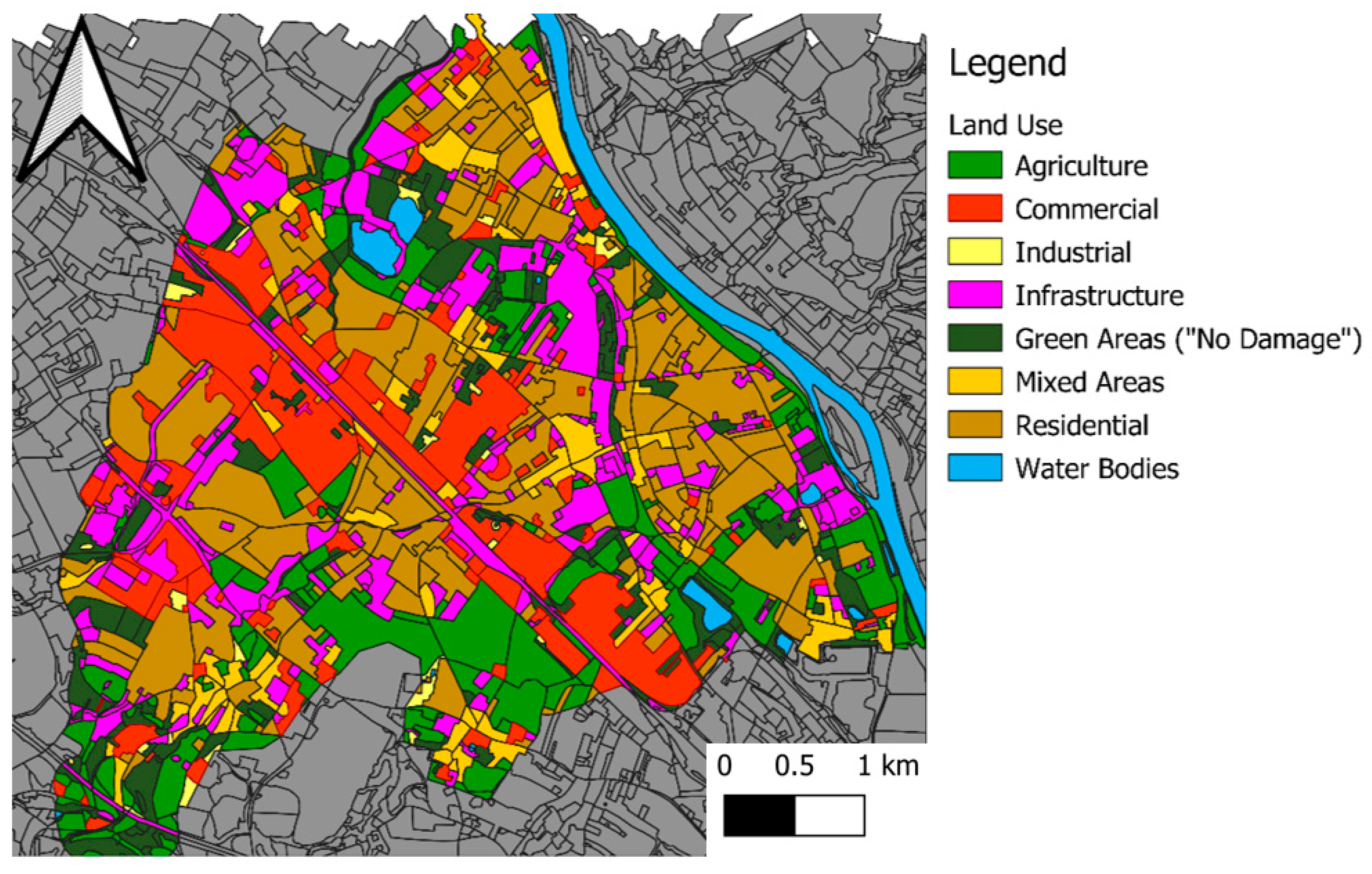
2.1. Study Area

For the present study, a subnetwork of the urban sewer system of Dresden, Germany is used. This network is located in the lower part of the Lockwitzbach subcatchment in the southeast of the city. Figure 1 shows the network, manholes, and a Digital Surface Model (DSM) provided by the State Service for Geoinformation and Geodesy of Saxony [22]. The drainage area equals 24.31 km², of which 42% is impervious, and it contains 8.4 km of the river before it flows into the Elbe River. The region has a variety of land uses seen in Figure 2, including residential, commercial, industrial, infrastructure, agricultural, different types of green areas, water bodies, and mixed areas [22].

2.2. Hydrodinamic Sewer System Model

In order to predict the extents and volumes of flood in urban areas, an array of tools and models exist. For this study, a combination of models will be used. Initially, hydrodynamic modeling of the sewer network is done using the United States Environmental Protection Agency’s (EPA) Storm Water Management Model (SWMM) [21]. This software model can simulate rainfall-runoff processes, infiltration, evaporation in the subcatchments defined in the model, and hydraulics in the sewer system as either kinematic or dynamic wave flow routings [21]. The dynamic wave uses the Saint-Venant flow equations to estimate gradually varied and unsteady flow [21].

A model calibrated for dry and wet weather flow of the Urban Drainage Network in SWMM of the Lockwitzbach area is used [23]. Historical data were used for calibration and validation, achieving values higher than 0.65 and 0.72 for Nash Sutcliff Efficiency, 0.71 and 0.92 for Klingt–Gupta Efficiency [23]. Different synthetic rainfall events were used as an input to the model, these are taken from the KOSTRA Atlas for the city of Dresden [24]. The KOSTRA Atlas rain events are used for dimensioning sewer systems and other stormwater infrastructure in Germany [24]. Using the Atlas, one-hour design storm events are produced using Euler type II [25] hyetographs with return periods of 10, 20, 50, and 100 years, which are based on reference precipitation intensities for the city of Dresden, Germany.

These events exceed the capacity of the sewer system and lead to a surcharge of the network. As a result, the sewer system overflows at the manholes, which are sources of flooding. The flood volume at the nodes, or manholes, is used as input for the next part of the process. Using the R package swmmr [26], a time series with steps of 5 min is extracted for each node that presents a flood surcharge through the manhole.

2.3. Interactive Tool within Agent-Based Model

The Agent-based Model (ABM) is developed in the software GAMA, which stands for GIS Agent-based Modeling Architecture [10]. It is used to simulate the propagation of inundation on the surface and to assess its impacts.

Moreover, different risk reduction measures are implemented in the tool, in which the user can decide location and other parameters in an intuitive manner. The results are visually compelling with options in 2 and 3 dimensions (2D and 3D) [10], which can lead to a more effective process in knowledge transfer [27].

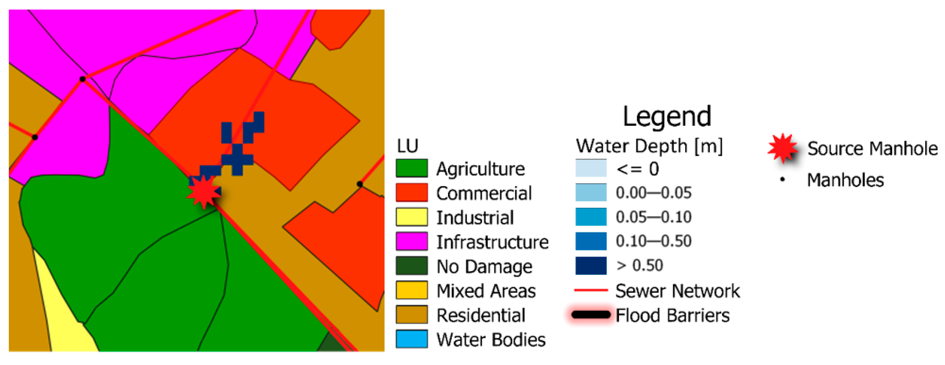
2.3.1. GIS-Based Overland Diffusive Algorithm

A GIS-based overland diffusive algorithm developed by Chen [7] is used to simulate the propagation of inundation. The model has been tested and compared to other 2D flood propagation models, leading to agreeable results for propagation areas and depths. The DSM is loaded into the software GAMA, which will be used to simulate the surface diffusion of floods. Furthermore, the DSM was pre-processed for sinks to allow a better diffusion. The approach by Chen consists of allocating the flood volume from SWMM as an attribute of the grid agent. Each cell can additionally be considered as a storage unit, with a capacity of 0.05 m of water depth. When this capacity is exceeded, the cell becomes a “source” cell. It is here the topography plays an important role, as water will only flow into the 8 adjacent cells, where their elevations allow it; meaning it will only diffuse towards the cells with lower elevations than the original source cell. The model will divide the flood volume among the relevant cells by making their depths equal. The process repeats on a loop if the border cells have a higher volume than the storage capacity of 0.05 m and if topography allows it. The process continues by now turning the nine cells (the eight adjacent cells and the original source cell) into the source or center and the volume flows into the next 16 adjacent cells.

For this work, the algorithm is repeated at each time step. Instead of only doing it for the total flood volume, this process is repeated for each source cell at each time step. The total flood volume is updated from the time series extracted in step 2.2 in SWMM. Thus, taking advantage of the dynamic capabilities of GAMA, in which the simulation can be continuous or step by step, leading to a dynamic urban flood model.

2.3.2. Assessment of Impacts

For the assessment of impacts, Land Use shape files from the Saxon State Ministry for Energy, Climate Protection, Environment and Agriculture [22] are loaded into GAMA. Along with these Land Use, the Global Depth-Damage Functions (DDF) by Huizinga [19] are also implemented. These damage functions are related to typical land use (LU) or land cover (LC) classes and estimate damage according to inundated area and depth. The damage function classes used for this study are residential, commercial, industrial, infrastructure, mixed areas, and agriculture. Other green areas are considered as no damage areas. Since the land use classes do not precisely match the damage function classes, the LU classes are assigned with the DDF that most closely fits the description [28]. For the mixed area, a combination of the residential and commercial Damage functions will be considered with equal ratios. The DDFs, were corrected for inflation using the methodology described in the same publication [19].

In the same manner that the propagation of damages can be monitored with GAMA, the accumulation of damages is monitored as well. As the diffusion of the flood volume takes place, the damage is calculated every step of the simulation by using the DDFs combined with the depth and area of inundation calculated using Chen’s method from step 2.2.1.

2.3.3. Flood Mitigation Measures in ABM

To show the versatility of the tool, the installation of temporary flood barriers is simulated. This flood mitigation measure is chosen because it requires the simulation of people as agents installing the barriers. The simulations can be visually explored and analyzed in a way that the user can modify the parameters to improve or compare results of simulations. Moreover, the installation of the barriers occurs as the flood propagation takes place. This allows also to exploit the dynamic capabilities of the tool.

The flood barriers are installed by agents according to the barriers manufacturer’s specifications. A different amount of installers and lead time before the rain event can be tested and selected by the user. The user can also select the location and height of the flood barriers by clicking where they want the barriers to be installed or test different preselected scenarios.

Initially, an additional two hours before the event and ten pairs of agents are used for the simulations to allow the agents to travel to the designated area to install the flood barriers before and during the early stages of the event. The lead time is chosen because forecasts for this type of extreme event exist in Early Warning Systems for pluvial urban flooding for two or more hours [29,30] and to ensure that the maximum amount of damage prevention happened. Since we have a rate for the instalment of the barriers, we can easily calculate the number of people needed to install them with a given lead time of two hours using Equation (1). On the other hand, if the amount of people available to install is a limited resource, the time needed before an event can also be calculated using Equation (2). The values shown are for the lead time of two hours and ten pairs of installers available.

Installers = L/(R × t) = L/((60 m/(pair∙h)) × (2 h)) = L/120,

(1)

t = L/(R × Installers) = L/((60 m/(pair∙h)) × (10 p)) = L/600,

(2)

where:

Installers = Pair of people or agents installing the flood barriers [pair];

L = Length of barriers in meters [m];

R = Rate of instalment, which is 30 m per person per hour [m×pair-1×h-1];

T = time in hours [h].

Conversely, with the dynamic and interactive capabilities of the ABM, the amount of time or people can be tested more accurately because the progress of the flood can be observed, and therefore, not all the barriers must be installed in advance. The model can take into account the time for the agents to travel from storage into position, plus the time it takes to change direction, to install the barriers, and then the time needed to move to the next spot where they will set the barriers, none of which is otherwise considered in the equations. For these simulations, an average speed of 10 km/h was considered for the agents. This means that different scenarios of lead times and number of installers can be explored using this approach. GAMA offers the capability to run exhaustive simulations without a display to run them faster while still outputting all the results into the different files [10]. The exhaustive simulations will be performed by setting minimum and maximum values for the lead time and number of installers and will give an increment to each parameter by a definite amount in every simulation. For the lead time, a minimum of 30 min and a maximum of two hours is used with 15-min increments. For the number of installers, a minimum of two pairs of people and a maximum of ten is used with increments of one pair at a time, totaling 63 simulations for each node. These results can then be compared with the baseline value of maximum reduction achieved by having the barriers set up in time to minimize flood propagation.

3. Results

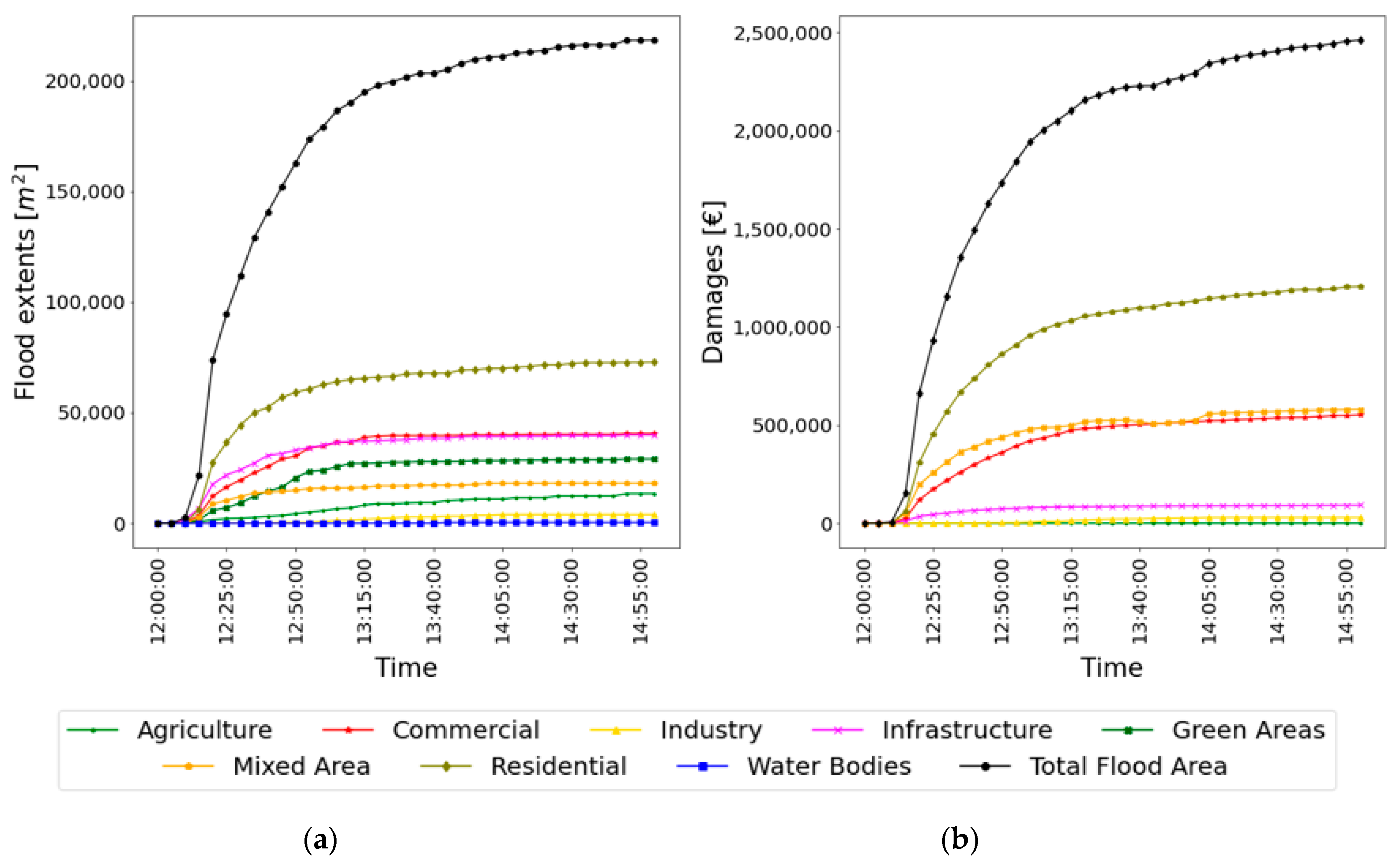
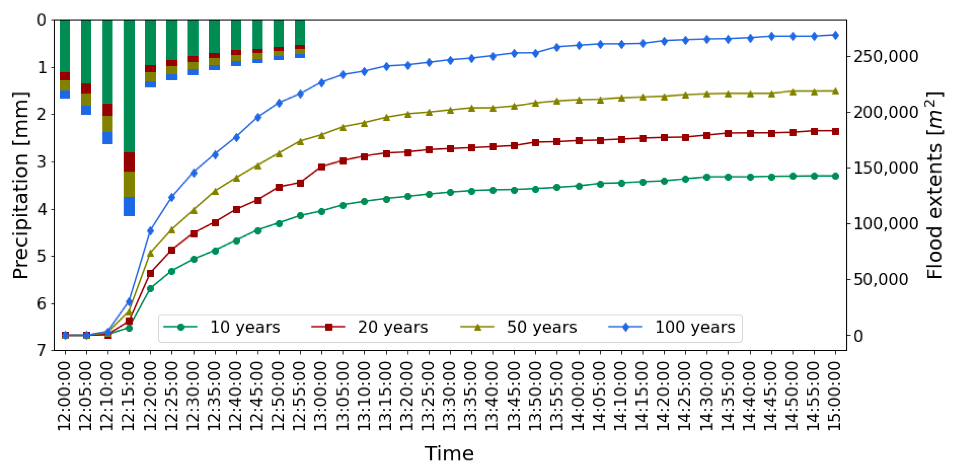
3.1. Flood Propagation and Its Impacts

Running a simulation in GAMA allows to follow the propagation of inundation in real-time, along with its impacts. This can be monitored in a variety of ways, like the display or a graph with the time series for both propagation of flood and the estimation of damages. The time series of both can be seen in Figure 3. In the figure, a series for each type of land use can be seen for the propagation of inundation. It should be noted that the simulation can be run continuously or step by step. This allows for a more detailed and dynamic analysis of the progression of the event and potential interventions at different stages, some of which will be further discussed below.

The model outputs *.csv files with the values for the propagation obtained directly from the raster as totals, as well as the flood volume of each manhole. Other outputs include raster files of flood depths and total damages, as well as *.kmz files to visualize the animated results in Google Earth [10,31].

In Figure 4, the total flood propagation of the four return periods can be observed in a graph along with the hyetographs of rain events used for the simulations. As expected, the longer the return period, the more widespread the flood becomes. Additionally, for all return periods, 50% of the flood propagation occurred within the first 30 min, even though some propagation still occurs until the end of the simulation, even a few hours after the rain event finished. This suggests that early action is needed to really decrease the propagation. As previously mentioned, a timely Early Warning System could provide up to a few hours of lead time in an urban environment [29,30].

Figure 5 shows the total flood extents of a 100-year return period event. These results are exported in a variety of ways. The results in the figure are from a raster image. Moreover, a file with discretized values of depths and inundated areas by the land use affected is also created. Finally, the inundated area created by the flood volume contributed by each manhole is also obtained. These values are also discretized by the land use affected.

Figure 6 shows the propagation of inundation according to Chen’s algorithm at different stages of the process. These close ups show that the size of every cell is more noticeable, which is ten by 10 × 10 m², meaning the cell has an area of 100 m². The flood volumes are divided by that area, resulting in a water depth represented by the blue colors according to the legend. The early effects of the flood are also visible since there is a lot more inundation happening in the first hour of the event compared to the next steps. In the first 30 min, 50% of the flood extent already took place.

As described in Section 2.3.2, the damage is estimated in real-time as the flood extents are propagating in the simulation. Figure 7 shows the damage for the same sample area as Figure 7. The differences in damages according to different DDF and LU is clearly visible in the raster. Even the “no damage” area is noticeable. Similar to propagation, most of the damage occurs in the early stages of the simulation.

3.2. Flooding and Its Impacts According to Manhole Distribution

The model only considers the manholes as flood sources because they represent the main source of flood volume in an UPF [7]. The model outputs the flood extent by source, or manhole. This means that the flood extent and its impacts contributed by each manhole can be discretized. In all return periods considered, only 10 manholes account for 40% of the total flood propagation. In addition, 17 nodes account for 50% of the total damage estimated by the model. This suggests that localized interventions to or around these manholes can have significant positive effects.

Table 1. Flood extent and damage by manhole contribution and land use.

Node Name	Inundated Area [m2]	Final Depth [m]	Residential Damage [€]	Commercial Damage [€]	Infrastructure Damage [€]	Other LU Damages [€]	Total Damage [€]	% of Total Damage
17L141	4700	0.28	158,083	-	-	-	158,083	5.08%
17Q108	14,200	0.05	-	136,398	2259	-	138,658	4.45%
38B140	1700	0.74	30,394	96,818	-	4	127,217	4.09%
17G25	30,600	0.05	10,863	89,500	22,284	-	122,647	3.94%
17H120	11,400	0.05	104,937	8165	-	-	113,103	3.63%
38G6	4700	0.09	1119	7435	-	88,431	96,986	3.12%
38F65	1500	0.18	6704	-	-	75,049	81,753	2.63%
39K169	12,400	0.05	58,352	-	12,672	-	71,024	2.28%
17Q49	4300	0.07	58,835	5107	472	-	64,414	2.07%
39P1	3900	0.05	28,509	-	-	33,555	62,064	1.99%

shows the manholes that contributed more to financial damages according to the model.

3.3. Flood Barriers

Using the results of contribution to damage by manhole for every return period, the nodes with higher contribution and their damaged areas were visually inspected. Different manholes are then selected visually for the application of flood barriers taking into account the topography, flood propagation, and land use in the flooded area. To visualize why this is the case, Figure 8 shows manholes and the flood propagation around them with and without flood barriers.

Manholes “17G25”, “39K169”, and “17H120” are selected because of the proximity to areas where no damage or low damage is considered. Noticeably, the flow of the inundation is mostly in that direction, meaning that topography could help to redirect or limit the flood extent to those areas. It is immediately apparent that the flood propagation was contained in the green areas with the flood barriers. Additionally notable, the flood depths are higher.

The case of manhole “38B140”, shown in Figure 9, contrasts with the previous ones. In this case, the topography of the area inevitably will lead the flood volumes towards the commercial land use. meaning that redirecting the flood to the lower damage areas would be not possible or impractical. This suggests that for this area, another type of flood mitigation measure would be more effective.

Simulations for manholes “17G25”, “39K169”, and “17H120” were carried out for each return period.

Table 2. Flood extents for manholes with and without flood protection barriers for all return periods in m².

	17G25			17H120			39K169
Return Period	Without Flood Barrier [m2]	With Flood Barrier [m2]	% Reduction	Without Flood Barrier [m2]	With Flood Barrier [m2]	% Reduction	Without Flood Barrier [m2]	With Flood Barrier [m2]	% Reduction
10-year	18,682	6394	65.78%	3696	3796	−2.70%	6294	2098	66.67%
20-year	22,778	6394	71.93%	5994	4695	21.67%	8492	2098	75.29%
50-year	28,473	6394	77.54%	8392	4695	44.05%	10,989	2098	80.91%
100-year	30,427	6394	78.99%	11,389	4695	58.77%	12,388	2098	83.06%

and

Table 3. Damage estimation for manholes with and without flood protection barriers for all return periods in Euros [€].

Return Period	17G25			17H120			39K169
	Without Flood Barrier	With Flood Barrier	% Reduction	Without Flood Barrier	With Flood Barrier	% Reduction	Without Flood Barrier	With Flood Barrier	% Reduction
10-year	122,778 €	10,191 €	91.70%	45,328 €	34,996 €	22.79%	34,384 €	11,156 €	67.55%
20-year	143,473 €	12,169 €	91.52%	53,266 €	39,616 €	25.63%	48,738 €	12,556 €	74.24%
50-year	178,560 €	14,481 €	91.89%	77,815 €	49,079 €	36.93%	60,538 €	14,608 €	75.87%
100-year	212,148 €	16,562 €	92.19%	116,171 €	59,891 €	48.45%	71,024 €	15,880 €	77.64%

show the changes in flood propagation and damages, respectively. Manhole “17H120” has an increase of flood extents for the return period of 10 years. This happens because water is routed to an area where more propagation with lower depths is possible. It is important to note that nonetheless, a damage reduction was observed in the model.

For these manholes, reductions in both flood extents and flood damages are very successful according to the simulations. Reductions in damages larger than 90% are seen in manholes “17G25”. As previously mentioned, these manholes are some of the largest contributors to damage in the model. However, localized actions around these manholes have important reductions in UPFs’ extensions and damages. Moreover, it is possible to visualize and explore options for the locations and parameters of the installations of the barriers in the tool.

Agents and Time Needed to Install the Flood Protection Barriers

Using Equation (1), the number of people needed can be calculated assuming a lead time before the event. Likewise, with Equation (2), we can calculate the amount of time needed for instalment of barriers previous to the start of the rain event by assuming a determinate amount of people available. Results for this approach are in

Table 4. Time and people needed for the instalment of flood protection barriers.

Manhole	17G25	17H120	39K169
Length of flood barrier needed in m	270.71	227.26	185.76
Pairs of installers for 1 h of lead time	5	4	4
Pairs of installers for 2 h of lead time	3	2	2
Time for 5 available pairs of installers in hours	0.90	0.76	0.62
Time for 10 available pairs of installers in hours	0.45	0.38	0.31

.

Nevertheless, these values can be calculated in a dynamic simulation because we can observe the progress of the inundation and the barriers can be installed in the order the barriers are needed as the propagation of flood is taking place. Even though this can save some time or people needed, the model in GAMA also considers the amount of time people needed to get in place and start installing the barriers. Having established the baseline values for reduced damage with the flood protection installed, the exhaustive simulations were performed to the three nodes where the barriers were installed. As seen in

Table 5. Pairs of flood barriers installers needed to reduce damage costs for 100-year return period events.

Manhole	17G25		17H120		39K169
Lead Time in Minutes	Using Equation	Using GAMA	Using Equation	Using GAMA	Using Equation	Using GAMA
30	9	11	8	5	6	8
45	6	6	5	4	4	5
60	5	5	4	3	3	4
75	4	4	3	3	2	3
90	3	4	3	2	2	3
105	3	3	2	2	2	2
120	2	3	2	2	2	2

, most of the results required additional people or time to install the flood barriers compared to the equations, albeit not all of them. For node “17H120”, with a lead time of 90 min, fewer pairs of people are needed to install the flood protection on time. These times could also vary with the location of the manhole in the catchment. Considering that could lead to better strategies and can also be analyzed. Other parameters that could be tested for this approach could be the rate at which different types of flood protection barriers are installed.

4. Discussion

Using Chen´s method in an ABM brings many capabilities and possibilities. Nevertheless, the limitations and omissions must be acknowledged. Whereas other models might be more accurate in representing the hydraulics of surface waters, they are also much more time-consuming because they require much more computational resources [5,7,8]. This also means that Chen’s method, and other GIS based methods, could be scalable to larger areas [7].

Even though the accuracy of Chen’s model has been validated and proven adequate for flat urban areas, the method neglects many processes. For example, it neglects several critical hydrodynamic processes and thus may not be suitable for all types of topography [7]. Flood velocities are notably neglected, which is why it may not be useful in areas with steep slopes. Current research is undergoing on that topic [7]. Another process not considered is the reintroduction of flood volume into the manholes once the capacity of the sewer system is restored after a precipitation event. This may lead to an overestimation of flood volumes in the areas around the manhole. Nonetheless, the area around it was also considered to be dry previous to the outflow through the manhole, neglecting the possibility that there might have already been water accumulated from precipitation.

However, manholes are the main contributors to flood volume during an UPF [5,7,8]. Although the effects are well documented, they are not entirely understood [8]. Therefore, it is justified to consider interventions to and around manholes to reduce flood risk in an area. The analysis performed on a few nodes allowed to get much insight into the potential financial damage reduction. The interactive tool in an ABM allows for an exploration of these measures, and for a compelling visual representation. These representations could be suitable for different stakeholders and not only experts.

The lack of interaction between inundations from different manholes is also notably neglected. The propagation of flood volume around a manhole is calculated for each manhole alone. This leads to a considerable overestimation when analyzing the results of the manholes contribution because overlapping flooded raster cells are calculated twice or more times. On the other hand, an underestimation occurs when analyzing the results directly from the raster or the complete time series.

Table 6. Differences in results for manhole contribution and final raster values.

Return Period	Flood Area [m2]		Damage Estimation [€]
	Manhole Contribution	Final Raster Values	Manhole Contribution	Final Raster Value
10	145,164	142,566	1,624,959	1,575,603
20	187,624	182,828	2,213,519	2,094,293
50	224,490	218,395	2,569,950	2,461,961
100	278,194	268,646	3,112,808	2,981,186

shows the difference in results for both approaches. The differences are substantial enough to consider since they approach values between 3% and 5% of difference.

The damage estimation is easy to implement and fast to calculate. Nonetheless, there is much uncertainty applying such broad DDFs to large areas [20,20,32,33]. DDF are assigned by land use, and in the case of this study, is an average for the whole country. LU types that could be further subdivided into classes, or DDF, can be developed for the study. More accurate methodologies could be applied in the same platform, like more region-specific DDFs or even building-specific DDFs. Sometimes in-depth data for the study area are not available. Therefore, as a starting point, the global DDFs used in this study can be used as a starting point to evaluate the consequences of urban floods [19]. Land use or land cover can be obtained from satellite images like Land from the COPERNICUS project [34]. Satellite datasets could be a great starting point to delineate areas of risk in large areas or cities, to select areas of interest for more in-depth studies.

Further approaches for the overland inundation method could potentially be implemented into an ABM. For example, a tighter coupling of the hydrodynamic sewer model and the overland diffusion. This could allow consideration of the reintroduction of water into the sewer system and the hydrostatic pressure effects of ponded areas above manholes [8]. The approach proposed by GebreEgziabher and Demissie considers interactions between overland and underground systems and also the interaction of multiple manholes inundations in the same area. That approach also has the advantage that it can model the recession of flood extents and thus can help for flood incident management after the event. Differential equations can be implemented in GAMA [10]. Therefore, other more sophisticated overland flow approaches for urban inundation could also be implemented, including two-dimensional overland models that consider flow velocities and their effects. However, these models would be significantly slower [5].

5. Conclusions

The proliferation of urban cover in the future is well established [35]. Pluvial urban floods will increase with the imperviousness associated with urban cover [3] and the effects of climate change will increase the frequency and intensity of high intensity rainfall events, reducing the return periods associated with them [4]. Consequently, approaches that can simulate large urban areas are necessary to assess vulnerability and risk. The complex interactions that take place before, during, and after a disaster event can be studied using tools like ABMs. This work presented a methodology to develop a model which couples a hydrodynamic model in SWMM with a dynamic and interactive ABM where a dynamic pluvial urban flood is simulated, and its impacts can be analyzed and monitored in real-time. The results were analyzed from the perspective of total flood extents and damage calculations. Moreover, the manhole contribution to flood and its impacts were analyzed and used to implement a risk reduction measure, namely flood barriers.

A noticeable characteristic of these events was that much of the propagation and its corresponding damage happens in the early stages of these incidents. The dynamic qualities of the ABM in GAMA allow for the monitoring of these instances. Although large lead times in warning systems are desirable, they are not always available. Therefore, knowing the extents of a flood at different stages and for different types of events can lead to better flood incident management. Another thing to note is that much of the inundation takes place in areas where the LU is typically associated with higher damages, namely residential and commercial areas. When analyzing manholes’ contribution, it was a small number of nodes that generated the majority of flood extents and damage. All of these suggests that early localized action can have large effects in minimizing the negative impacts associated with UPFs.

The instalment of flood protection barriers was selected as a measure to manage flood at a manhole level because it showcases the versatility and compelling visualization of the tool. Moreover, they can be used to study manholes as a source of flood volume and study localized actions. The manholes for study cases were selected for this purpose by analyzing Land Use and topography in its surroundings. In some cases, the flood barriers helped to decrease the damages of their surrounding area by values higher than 90%. In other cases, even though the flooded area increased due to the barriers, there were decreased damages in the area. The lead time of an Early Warning System and the number of people needed to install flood barriers to minimize damage were tested. Since both of these can be a limited resource, exhaustive combinations of dynamic simulations were performed and compared to the baseline values of flood extents and damages. Results varied depending on the manholes and return period, but most results indicated that more time or people was needed to install the barriers than what the barriers’ user manual specifies. Only one instance had a lower time and people requirement.

As previously mentioned, much of the flood propagation happens in the early stages of the event, meaning that although there is no need to have the flood protection in place before the event starts, for the barriers to be effective, early installation is vital. Using this approach, other kinds of barriers can be tested with variable heights and different strategies to install the barriers or where to install them can be researched. The user of the tool can also test different locations and parameters of this mitigation measure, which can lead to a better understanding of the system and knowledge transfer. Additionally, for an established Early Warning System, knowing the available resources, better flood incident management can be studied and carried out.

A significant advantage of using this approach is short computer processing times. The tool could also be used to evaluate different types of impacts. Environmental damages, loss of life, and other indirect damages could be studied within this approach. The advantage of having a faster model also leads to the conclusion that it is scalable. ABMs can be used at all scales, from houses to buildings, to neighborhoods, to large cities. In this context, other possibilities that can be researched in “real-time” at different scales are warning systems and evacuations [36]. Another applications for dynamic ABMs that can be combined with this approach is traffic congestion due to flood [12], which would benefit from the short computational times. Using ABMs, the propagation of information for flood incident management using tools like social media has been studied [37] and can be implemented. Moreover, other flood risk reducing measures could be implemented to the tool. For example, installation of retention tanks, infiltration swales, green roofs, porous pavements, increase of green and/or permeable areas, among others.

Methodologies for dynamic UPFs that can be scaled and easily applied are valuable tools for sustainable urban development, mainly where historical data or computational resources are scarce, like in some developing countries. There are substantial limitations to this type of simplified inundation model due to its assumptions and the uncertainty attached to them. As already mentioned, it may not be suitable for all areas, and it neglects a lot of relevant hydraulic processes. Nevertheless, case studies have shown that they can accurately estimate flood depths and extents for some applications [7], although more extensive testing is needed. Compared to other models that require larger datasets and computational power, the methodology presented in this research provides a good alternative for risk assessment in large areas. It is also a good option for appraising effects related to interventions to urban areas and development projects, and for testing potential measures and instruments for flood risk reduction.

References

1. United Nations. World Urbanization Prospects the 2018 Revision; United Nations: San Francisco, CA, USA, 2018. [Google Scholar]
2. World Bank Urban Development Overview. Available online: https://www.worldbank.org/en/topic/urbandevelopment/overview (accessed on 4 April 2020).
3. Jacobson, C.R. Identification and Quantification of the Hydrological Impacts of Imperviousness in Urban Catchments: A Review. J. Environ. Manag. 2011, 92, 1438–1448. [Google Scholar] [CrossRef] [PubMed]
4. IPCC. IPCC Climate Change 2014: Synthesis Report. Contribution of Working Groups I, II and III to the Fifth Assessment Report of the Intergovernmental Panel on Climate Change; IPCC: Geneva, Switzerland, 2014. [Google Scholar]
5. Bulti, D.T.; Abebe, B.G. A Review of Flood Modeling Methods for Urban Pluvial Flood Application. Model. Earth Syst. Environ. 2020, 6, 1293–1302. [Google Scholar] [CrossRef]
6. Wu, X.; Wang, Z.; Guo, S.; Lai, C.; Chen, X. A Simplified Approach for Flood Modeling in Urban Environments. Hydrol. Res. 2018, 49, 1804–1816. [Google Scholar] [CrossRef]
7. Chen, W.; Huang, G.; Zhang, H. Urban Stormwater Inundation Simulation Based on SWMM and Diffusive Overland-Flow Model. Water Sci. Technol. 2017, 76, 3392–3403. [Google Scholar] [CrossRef]
8. GebreEgziabher, M.; Demissie, Y. Modeling Urban Flood Inundation and Recession Impacted by Manholes. Water 2020, 12, 1160. [Google Scholar] [CrossRef]
9. Nkwunonwo, U.C.; Whitworth, M.; Baily, B. A Review of the Current Status of Flood Modelling for Urban Flood Risk Management in the Developing Countries. Sci. Afr. 2020, 7, e00269. [Google Scholar] [CrossRef]
10. Taillandier, P.; Gaudou, B.; Grignard, A.; Huynh, Q.-N.; Marilleau, N.; Caillou, P.; Philippon, D.; Drogoul, A. Building, Composing and Experimenting Complex Spatial Models with the GAMA Platform. GeoInformatica 2019, 23, 299–322. [Google Scholar] [CrossRef]
11. Dawson, R.J.; Peppe, R.; Wang, M. An Agent-Based Model for Risk-Based Flood Incident Management. Nat. Hazards 2011, 59, 167–189. [Google Scholar] [CrossRef]
12. Zhu, J.; Dai, Q.; Deng, Y.; Zhang, A.; Zhang, Y.; Zhang, S. Indirect Damage of Urban Flooding: Investigation of Flood-Induced Traffic Congestion Using Dynamic Modeling. Water 2018, 10, 622. [Google Scholar] [CrossRef]
13. Kasereka, S.; Kasoro, N.; Kyamakya, K.; Doungmo Goufo, E.F.; Chokki, A.P.; Yengo, M.V. Agent-Based Modelling and Simulation for Evacuation of People from a Building in Case of Fire. Proc. Procedia Comput. Sci. 2018, 130, 10–17. [Google Scholar] [CrossRef]
14. Terti, G.; Ruin, I.; Anquetin, S.; Gourley, J.J. Dynamic Vulnerability Factors for Impact-Based Flash Flood Prediction. Nat. Hazards 2015, 79, 1481–1497. [Google Scholar] [CrossRef]
15. Yang, L.E.; Scheffran, J.; Süsser, D.; Dawson, R.; Chen, Y.D. Assessment of Flood Losses with Household Responses: Agent-Based Simulation in an Urban Catchment Area. Environ. Model. Assess. 2018, 23, 369–388. [Google Scholar] [CrossRef]
16. Anshuka, A.; van Ogtrop, F.F.; Sanderson, D.; Leao, S.Z. A Systematic Review of Agent-Based Model for Flood Risk Management and Assessment Using the ODD Protocol. Nat. Hazards 2022, 112, 2739–2771. [Google Scholar] [CrossRef]
17. Chapuis, K.; Amine Elwaqoudi, T.; Brugière, A.; Daudé, E.; Drogoul, A.; Gaudou, B.; Nguyen-Ngoc, D.; Quang Nghi, H.; Zucker, J.-D. An Agent-Based Co-Modeling Approach to Simulate the Evacuation of a Population in the Context of a Realistic Flooding Event: A Case Study in Hanoi (Vietnam). In Proceedings of the Modelling, Simulation and Applications of Complex Systems, Penang, Malaysia, 8–11 April 2019; Volume 978. [Google Scholar] [CrossRef]
18. Dubbelboer, J.; Nikolic, I.; Jenkins, K.; Hall, J. An Agent-Based Model of Flood Risk and Insurance. J. Artif. Soc. Soc. Simul. 2017, 20, 6. [Google Scholar] [CrossRef]
19. Huizinga, J.; De Moel, H.; Szewczyk, W. Global Flood Depth-Damage Functions; JRC Technical Reports; Publications Office of the European Union: Luxembourg, Luxembourg, 2017. [Google Scholar] [CrossRef]
20. De Moel, H.; Aerts, J.C.J.H. Effect of Uncertainty in Land Use, Damage Models and Inundation Depth on Flood Damage Estimates. Nat. Hazards 2011, 58, 407–425. [Google Scholar] [CrossRef]
21. Rossman, L.A. Storm Water Management Model, User’s Manual, Version 5.1; National Risk Management Research Laboratory Office of Research and Development U.S. Environmental Protection Agency: Cincinnati, OH, USA, 2015. [Google Scholar]
22. Sächsisches Staatsministerium für Energie, Klimaschutz, Umwelt und Landwirtschaft. Biotoptypen- Und Landnutzungskartierung (BTLNK)—Sachsen.De. Available online: https://www.natur.sachsen.de/biotoptypen-und-landnutzungskartierung-btlnk-22282.html#a-22291 (accessed on 13 August 2020).
23. Reyes-Silva, J.D.; Bangura, E.; Helm, B.; Benisch, J.; Krebs, P. The Role of Sewer Network Structure on the Occurrence and Magnitude of Combined Sewer Overflows (CSOs). Water 2020, 12, 2675. [Google Scholar] [CrossRef]
24. Malitz, G.; Ertel, H. KOSTRA-DWD-2010 Starkniederschlagshöhen Für Deutschland (Bezugszeitraum 1951 Bis 2010)—Abschlussbericht; Deutsche Wetterdienst DWD: Offenbach, Germany, 2015; pp. 1–40. [Google Scholar]
25. Deutsche Vereinigung für Wasserwirtschaft, Abwasser und Abfall eV. Arbeitsblatt DWA-A 118; Deutsche Vereinigung für Wasserwirtschaft, Abwasser und Abfall e.V.: Hennef, Germany, 2006; ISBN 978-3-939057-15-4. [Google Scholar]
26. Leutnant, D.; Doering, A.; Henrichs, M.; Sonnenberg, H. Package “swmmr” Type Package Title R Interface for US EPA’s SWMM. 2020. Available online: https://cran.r-project.org/web/packages/swmmr/swmmr.pdf (accessed on 28 November 2022).
27. Opiła, J. Role of Visualization in a Knowledge Transfer Process. Bus. Syst. Res. J. 2019, 10, 164–179. [Google Scholar] [CrossRef]
28. Reyes-Silva, J.D.; Frauches, A.C.N.B.; Rojas-Gómez, K.L.; Helm, B.; Krebs, P. Determination of Optimal Meshness of Sewer Network Based on a Cost—Benefit Analysis. Water 2021, 13, 1090. [Google Scholar] [CrossRef]
29. Duncan, A.P.; Chen, A.S.; Keedwell, E.C.; Djordjević, S.; Savić, D.A. RAPIDS: Early Warning System for Urban Flooding and Water Quality Hazards. In Proceedings of the Machine Learning in Water Systems Symposium: Part of AISB Annual Convention 2013, Exeter, UK, 3–5 April 2013; pp. 25–29. [Google Scholar]
30. Golding, B.W. Review Long Lead Time Flood Warnings: Reality or Fantasy? Meteorol. Appl. Meteorol. Appl. 2009, 16, 3–12. [Google Scholar] [CrossRef]
31. Google LLC. Google Earth Pro; Google LLC: Menlo Park, CA, USA, 2020. [Google Scholar]
32. Wagenaar, D.J.; de Bruijn1, K.M.; Bouwer, L.M.; De Moel, H. Uncertainty in Flood Damage Estimates and Its Potential Effect on Investment Decisions. Nat. Hazards Earth Syst. Sci. Discuss. 2015, 3, 607–640. [Google Scholar] [CrossRef]
33. Freni, G.; La Loggia, G.; Notaro, V. Uncertainty in Urban Flood Damage Assessment Due to Urban Drainage Modelling and Depth-Damage Curve Estimation. Water Sci. Technol. 2010, 61, 2979–2993. [Google Scholar] [CrossRef] [PubMed]
34. Copernicus-Landuberwachungsdienst CORINE Bodenbedeckung. Available online: https://land.copernicus.eu/de (accessed on 25 June 2020).
35. Chen, G.; Li, X.; Liu, X.; Chen, Y.; Liang, X.; Leng, J.; Xu, X.; Liao, W.; Qiu, Y.; Wu, Q.; et al. Global Projections of Future Urban Land Expansion under Shared Socioeconomic Pathways. Nat. Commun. 2020, 11, 537. [Google Scholar] [CrossRef] [PubMed]
36. Shirvani, M.; Kesserwani, G.; Richmond, P. Agent-Based Simulator of Dynamic Flood-People Interactions. arXiv 2019, arXiv:1908.0523. [Google Scholar] [CrossRef]
37. Rand, W.; Herrmann, J.; Schein, B.; Vodopivec, N. An Agent-Based Model of Urgent Diffusion in Social Media. J. Artif. Soc. Soc. Simul. 2015, 18, 1–24. [Google Scholar] [CrossRef]
Figure 1. Digital surface model of study area with urban drainage network and manholes of study area in the Lockwitzbach subcatchment.
Water 15 00696 g001
Figure 2. Land use and catchment of urban drainage subnetwork of the study area in Lockwitzbach subcatchment.
Water 15 00696 g002
Figure 3. Time series of propagation of flood extents and its impacts for a 50-year return period design storm event. (a) Flood extents in [m2] (b) Damage estimation in [€].
Water 15 00696 g003
Figure 4. Time series of flood extents for design storm events for all return periods (10-, 20-, 50-, and 100- year).
Water 15 00696 g004
Figure 5. Total flood inundation extents and depths for a design storm event with a 100-year return period.
Water 15 00696 g005
Figure 6. Overland diffusion for a design storm event with a 50-year return period flood in GAMA in study case area. (a) Flood propagation 30 min after the start of rain event; (b) Flood propagation 180 min after the rain event started.
Water 15 00696 g006
Figure 7. Final raster for damages for a design storm event with a 50-year return period in GAMA.
Water 15 00696 g007
Figure 8. Final flood extents propagation in GAMA for different manholes of a design storm event with 100-year return period. (a) Manhole “17G25” without flood barriers; (b) Manhole “17G25” with flood barriers; (c) Manhole “39K169” without flood barriers; (d) Manhole “39K169” with flood barriers; (e) Manhole “17H120” without flood barriers; (f) Manhole “17H120” with flood barriers.
Water 15 00696 g008
Figure 9. Final flood extents propagation in GAMA for manhole “38B140” of a design storm event with 100-year return period.
Water 15 00696 g009