3.1. Application in Cambodia
The sampling technique with the mixed approach as described in
Section 2.4.3 worked best for Cambodia. The result of validating 25% of the data per station is shown in
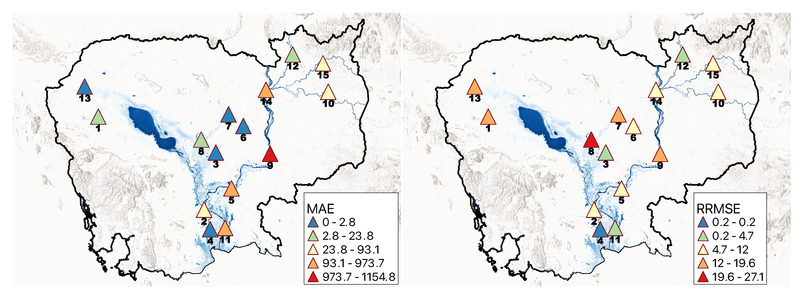
Table 5. The KGE was >96% for all stations. The MAE ranges from 0.6 to 1154.8 m
/s, with around 47% of the stations having a single-digit MAE, and 60% having a single-digit RRMSE. Since the KGE is high (>96%), we have only shown each station’s MAE & RRMSE values in
Figure 5.
Table 5 also presents the overall mean and standard deviation (SD) for each statistic. The model produced an average KGE, MAE, and RRMSE of 99.1%, 199.8 m
/s, and 10.8% respectively, with the average SD of 1%, 369.3 m
/s, and 7.6% for KGE, MAE, and RRMSE, respectively. Overall, the stations on the Mekong main river channel (Kompong Cham, Kratie, Neak Luong, and Stung Treng) had lower RRMSE (10.0%) than other stations (11.1%).
Additionally, we determined three levels of flows (high, medium, and low) for each stations. The high flow records were defined as the flows equal or above the 80th percentile flow (
) for the station; the low flow records were defined as the one equal or below the 20th percentile flow (
) for the station, and anything in between (
) was defined to be mid flow records. The MAE and RRMSE were calculated for each flow level from the discharge estimates for each station and shown in
Table 6, where the mean and SD for each flow are also shown. The MAE for the mid flow records was almost five and half times (5.4×) more that of the MAE for the low flow records, while the MAE for the high flow records was nearly three times (2.9×) of the mid-flow records. In contrast, the high flow records had the lowest RRMSE which was two and half times (2.5×) lesser than the low flow records. The mid flow records had the highest RRMSE which was more than two and half times (2.8×) than the low flow records.
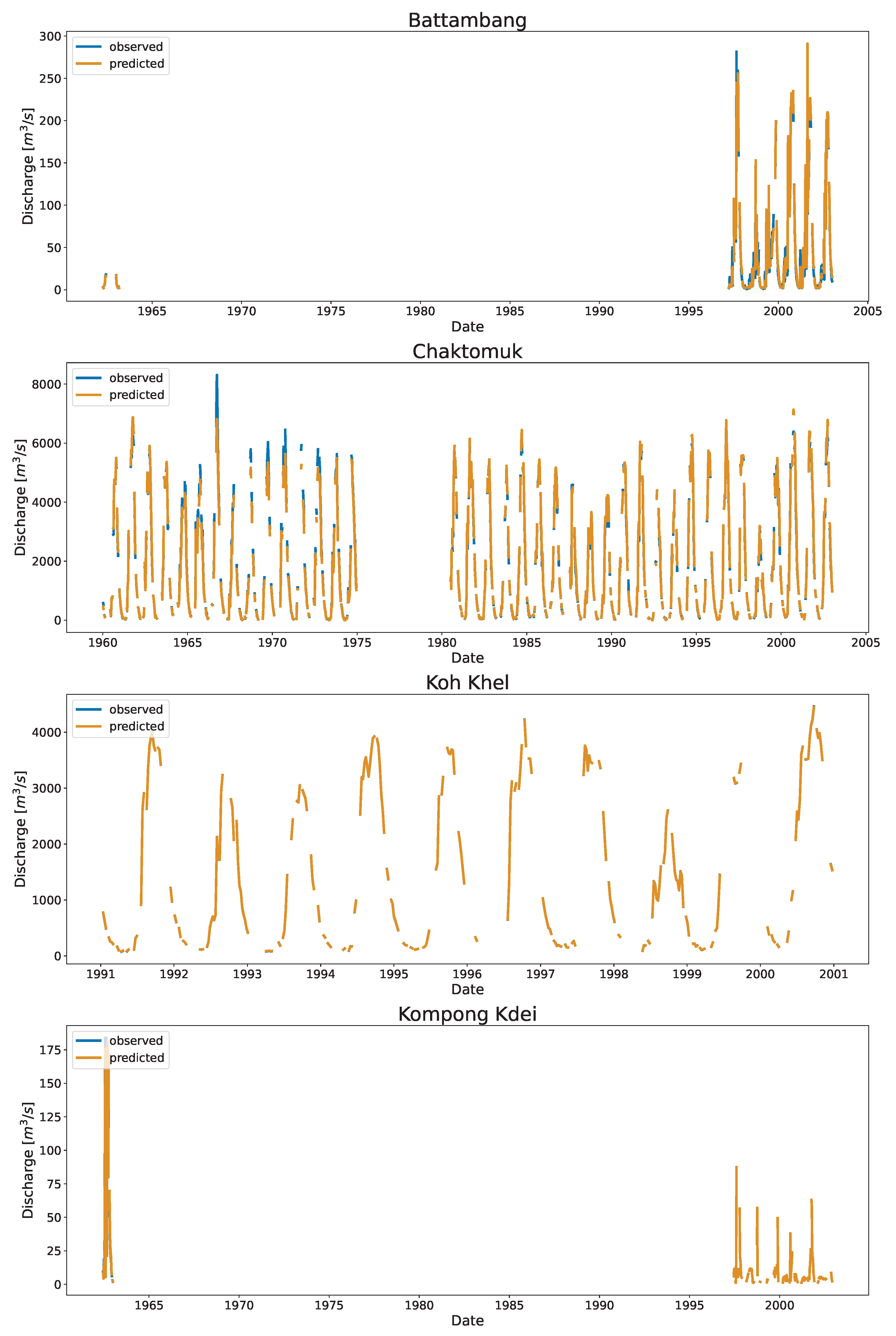
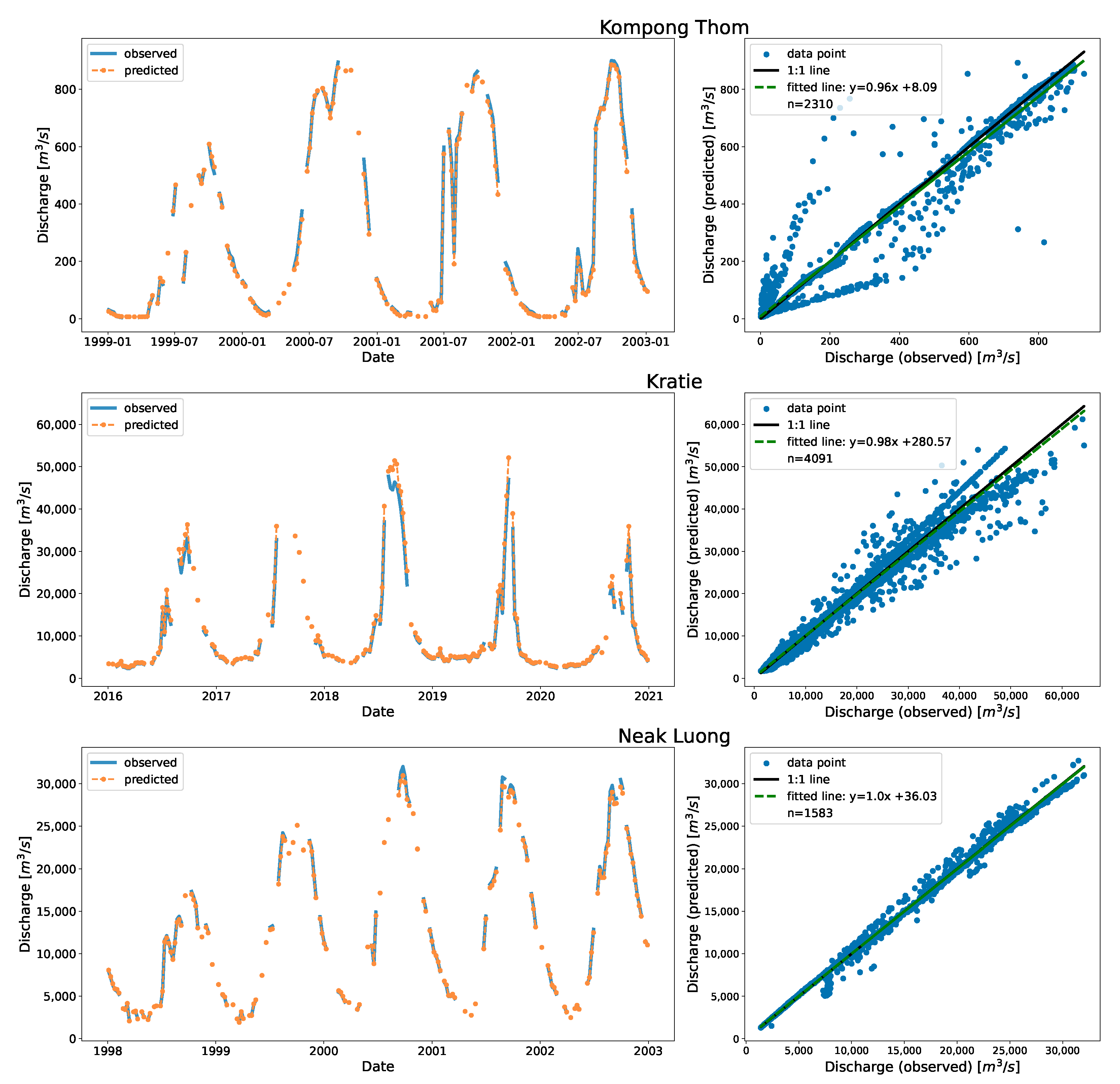
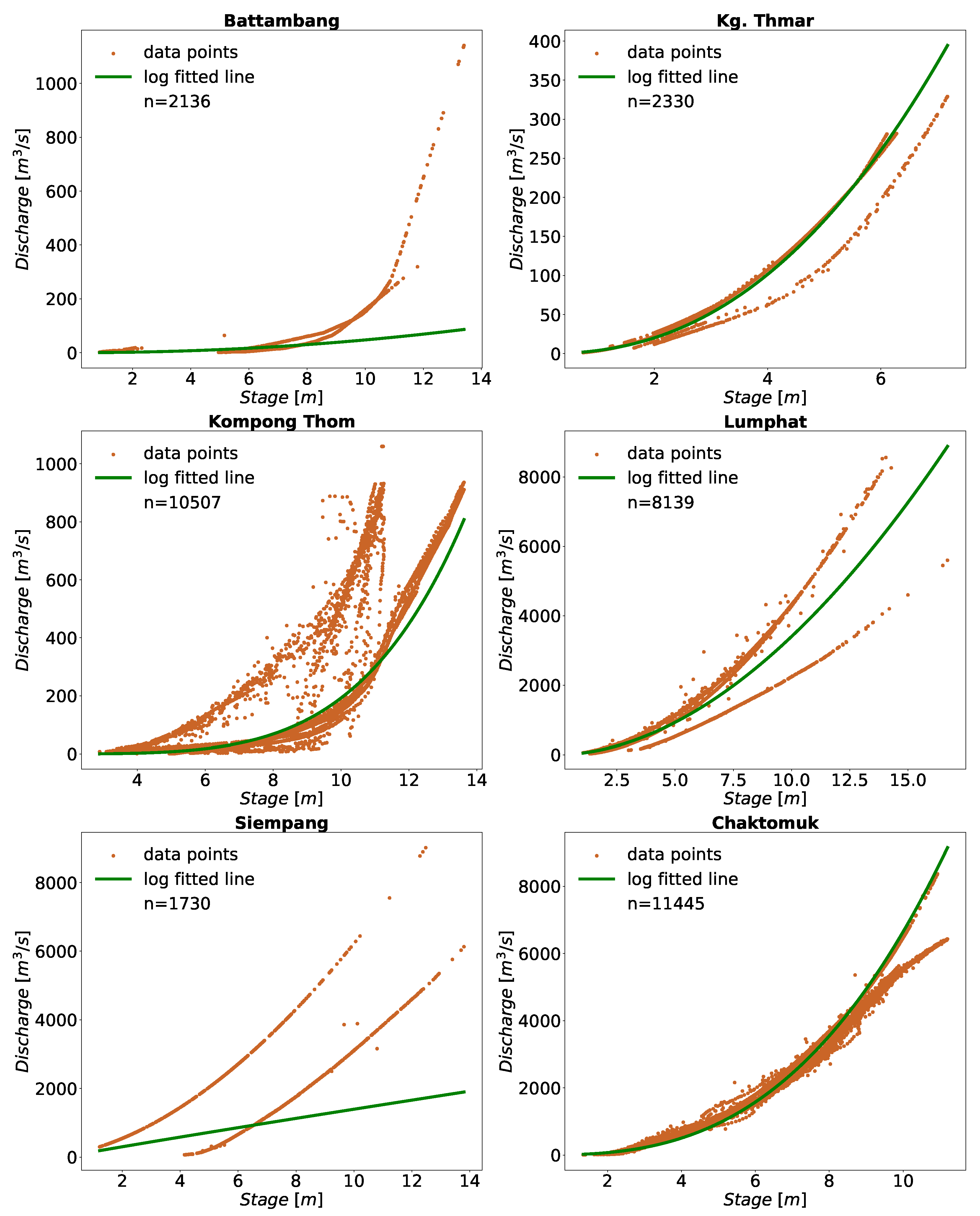
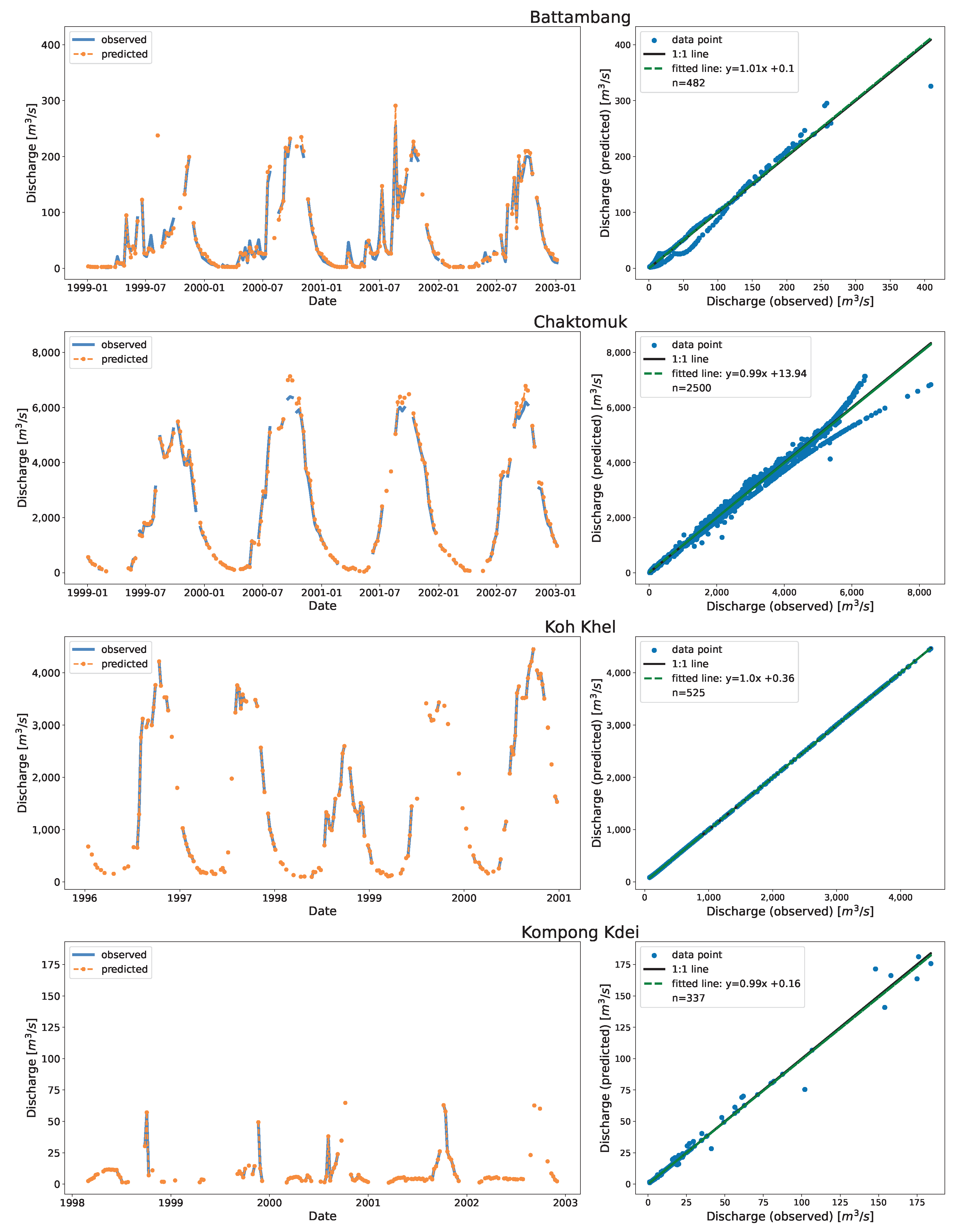
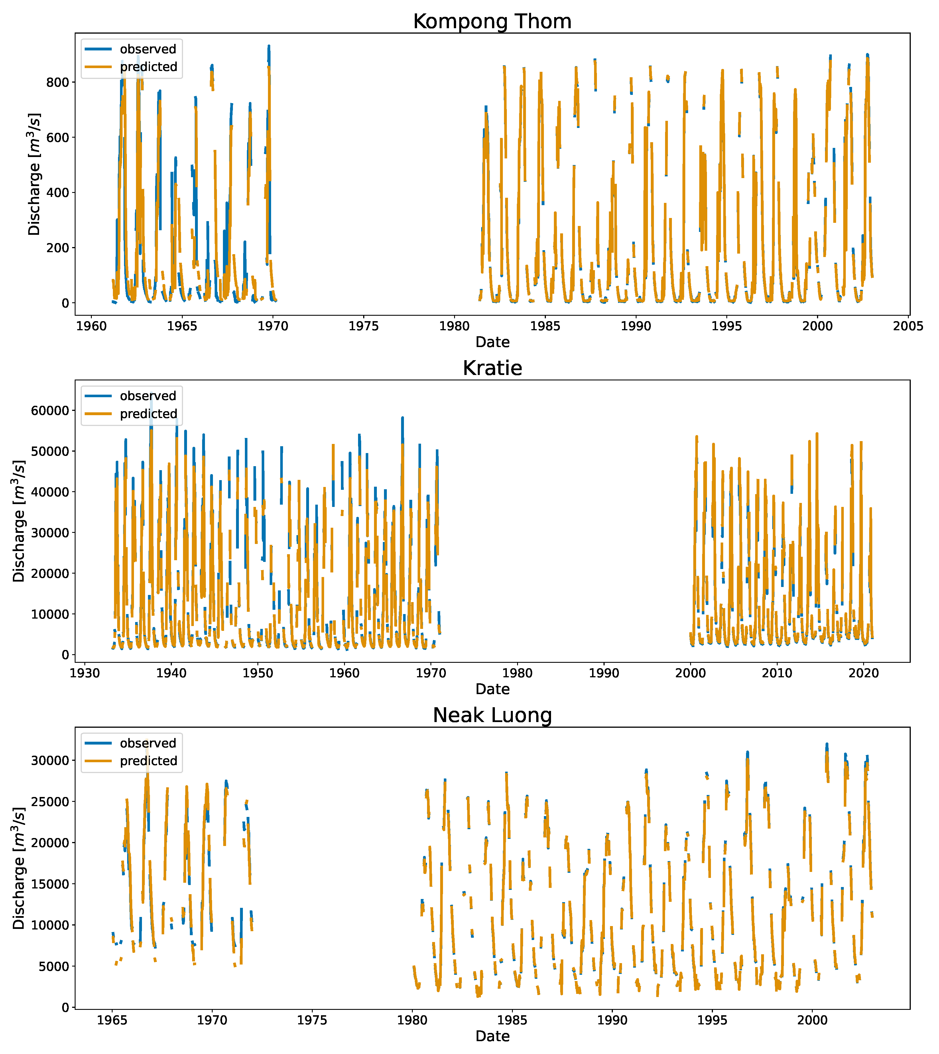
Figure 6 shows the time series and the associated scatter plots of the discharge as estimated using DDRC against observed data for Cambodia. The plot show the 1:1 line to highlight the differences between the simulated and observed streamflow data. The stations shown in
Figure 6 have stations affected by the overland flow of the TSL (Chaktomuk & Kompong Thom), and stations with range of discharge (Battambang, Kompong Kdei, Koh Khel, Kratie, & Neak Luong).
The scatter plot at Kompong Thom, which had the highest RRMSE, shows that the prediction was poor at the low end compared to the high end. There is a data gap between the years 1970 and 1982 (
Figure A1). The data gap could be due to Cambodia’s political instability because of Civil War [
59,
60]. Chaktomuk’s data appeared to have split into two ends at the high end. The model approximates the discharge by taking the values between two splits. The model at Neak Luong showed constant under prediction at low end before 1972 (Refer to
Figure A1). The base flow of Neak Luong before 1972 has changed from that after 1980, which may be due to the massive flooding that occured in 1978 [
61]. The clustering with time and stage as input features captured this variation. The model perfectly fits at Koh Khel (with KGE of 1.0). The station had a well-distributed dataset at low, mid, and high flow records.
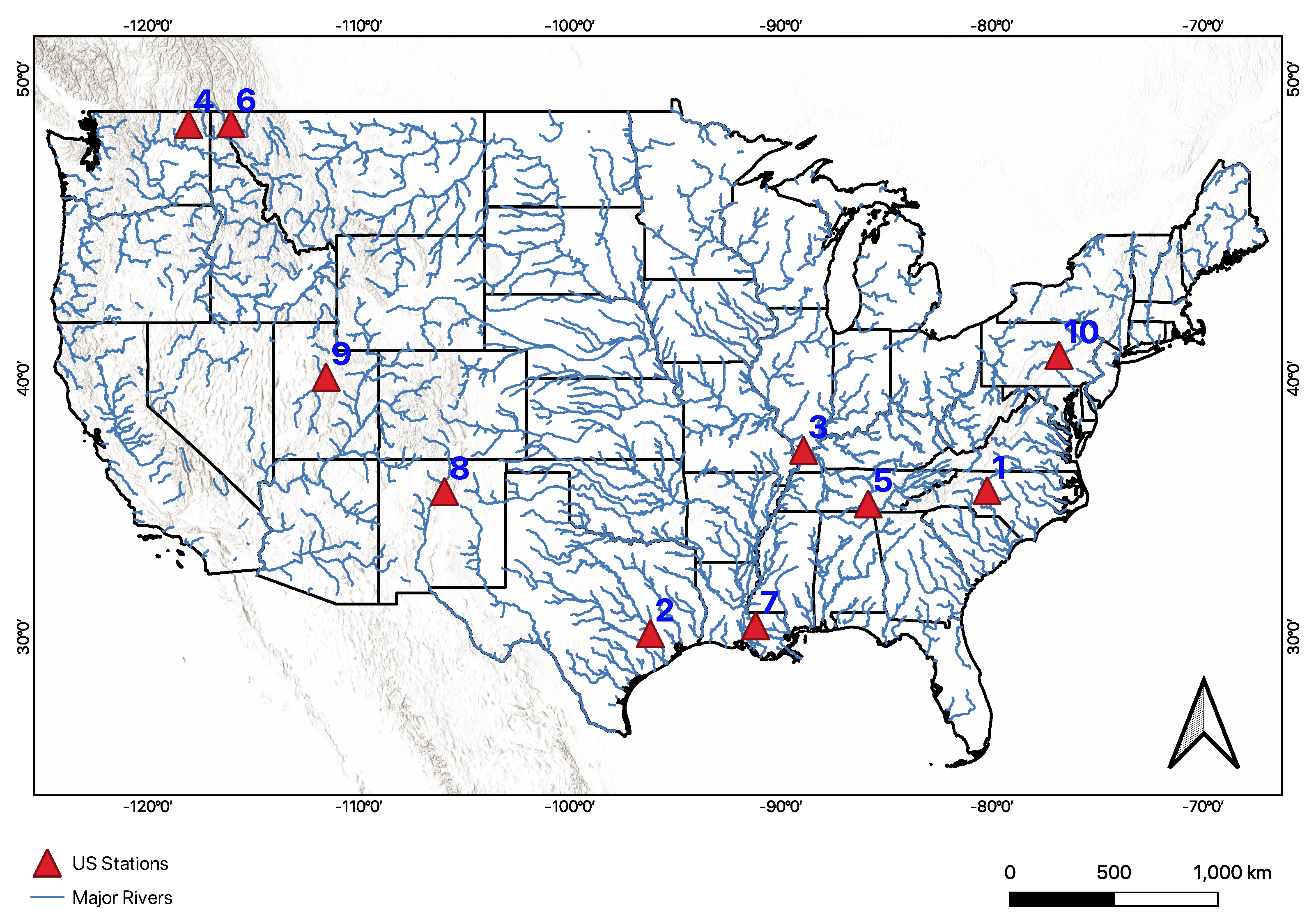
3.2. Application in the US
We applied the method to some stations in the US obtained from USGS. These stations were selected in random to represent range of flows. (e.g., Rio Tesuque below diversions near Santa Fe in New Mexico & Mississippi River at Baton Rouge in Louisiana).
Since USGS performs quality control on the data, we used ten years of data (2010 to 2020). The sampling technique with the mixed approach worked best for the US as well. The results of validating 25% of the data per station are shown in
Table 7. The KGE values are similar to Cambodia (>0.90 for all stations); the MAE had a lower range, for example, the Brazos River Near Hempstead (mean flow of 228.2 m
/s) had MAE of 10.50 m
/s, while a similar flow station in Cambodia, Kompong Thom (mean flow of 235.2 m
/s) had MAE of 23.83 m
/s. This could be because of the overland flow of water at Kompong Thom as discuss more later. A high-flow station in the US placed at the Mississippi river at Baton Rouge had lower MAE of 296.22 m
/s; the high flow station in Cambodia, Neak Luong which had MAE of 351.57 m
/s. This may be because of data quality especially the dataset before 1973 for Neak Luong.
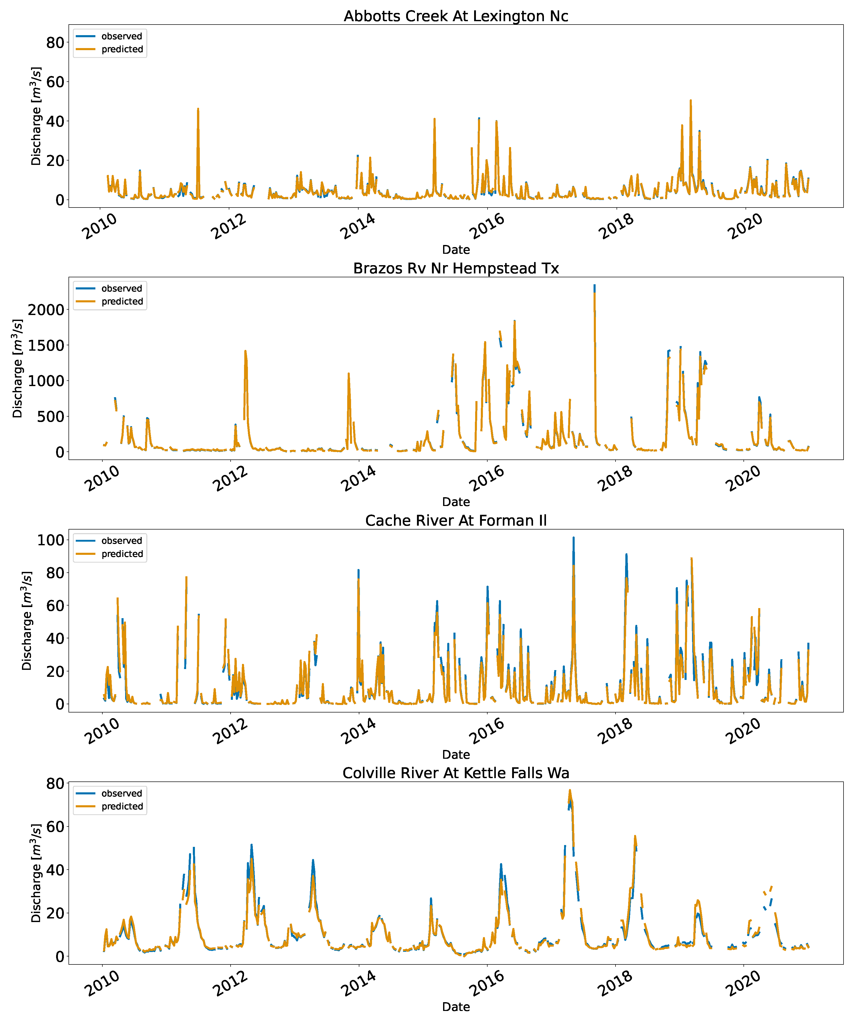
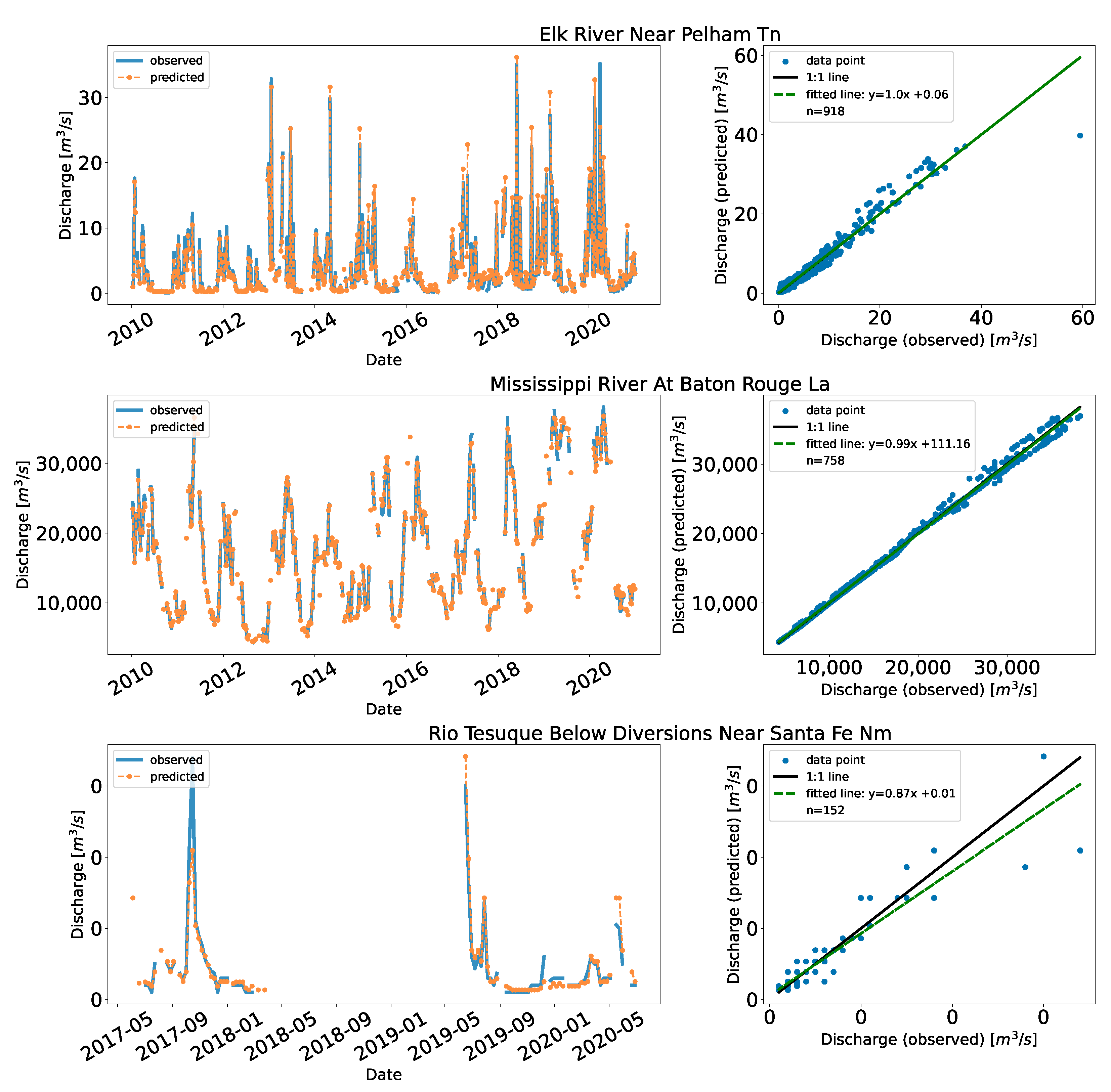
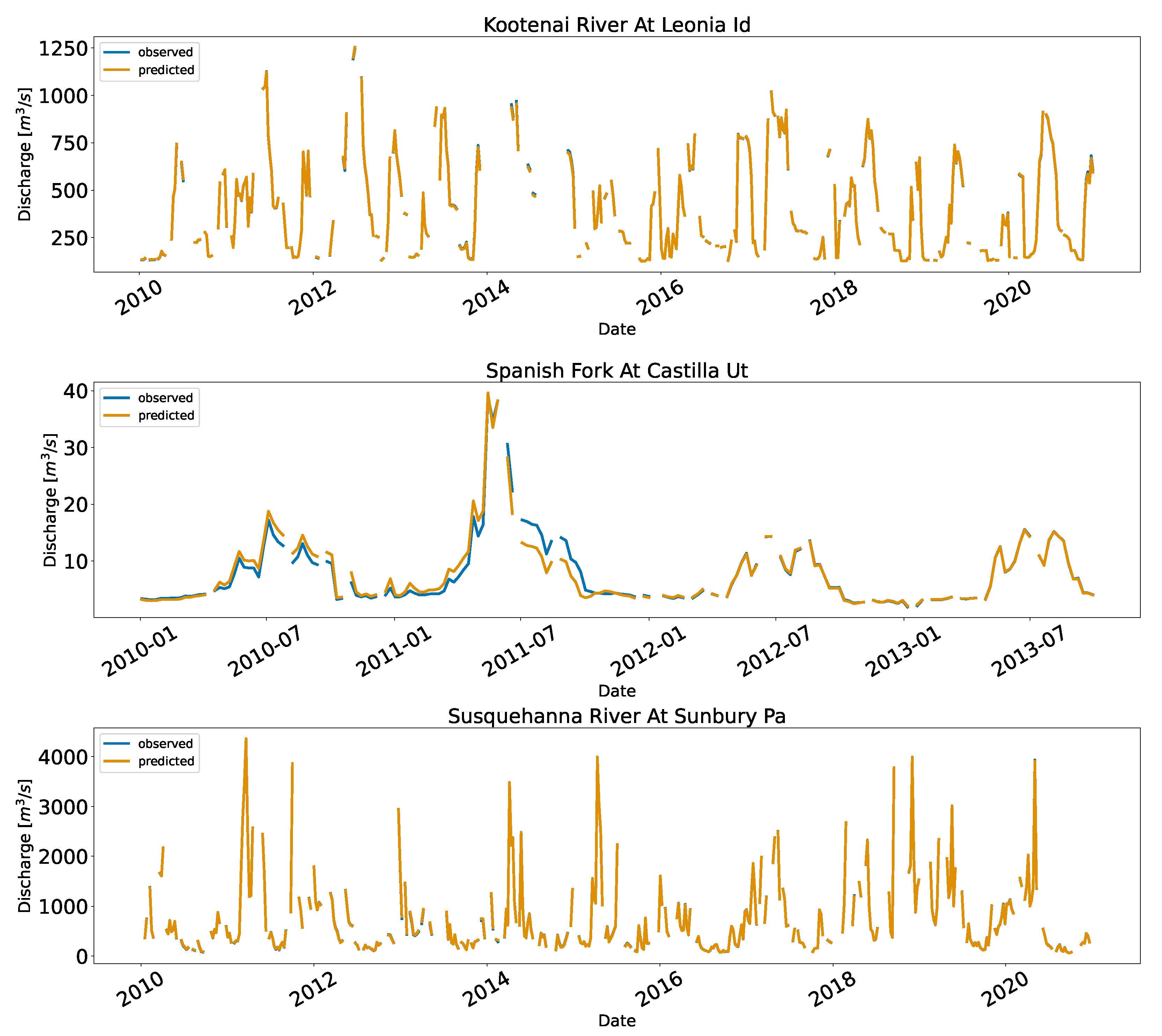
Figure 7 shows the time series and the scatter plots for the implementation in the US.
Similar to Cambodia, we determined three levels of flows (high, medium, and low) for each stations with the same definition, where the high flow records were the flows equal or above the 80th percentile flow (
) for the station, the low flow records were the one equal or below the 20th percentile flow (
) for the station, and anything in between (
) was defined to be mid flow records. The MAE and RRMSE of this analysis for each station is shown in
Table 8. The MAE for the mid flow records was almost twice (1.7×) that of the MAE for the low flow records, while the MAE for the high flow records were four times (4.0×) the mid flow records. In contrast, the high flow records had the lowest RRMSE which was almost one and half times (1.3×) lesser than the low flow records. The mid flow records had the highest RRMSE which was almost two and half times (2.4×) more than the low flow records.
3.3. Discussion
The analysis of results from both Cambodia and US stations suggest that the proposed method worked well across the regions. We used time-series information to understand the changes in the floodplain to generalize the RC. The method is scalable, automatic, and modular; choices for different routines in the methods can be switched, added, or removed.
Results showed that the high flow records had lower errors associated with them (
Table 3 and
Table 4) and was observed in both cases of the Cambodia and the US status. The practical implications for these results comparing high, mid, and low flow show that the DDRC method is better at predicting discharge from gauge height during high flow events (i.e., flood events). Conversely, during low flow events (i.e., Drought periods) the estimated discharge is shown to have a lower accuracy. This was also consistent with study by [
62] who used Gene Expression Programming (GEP) [
63] as a data-derived approach, and found that GEP was more reliable for extreme flood events.
Similarly, the distribution of the data points affected the performance. The Rio Tesuque station near Santa Fe in New Mexico had lower KGE (90.9%) and highest RRMSE (39.1%) than other stations. The fitted model was under predicting which is evident by the slope of the fitted line (0.87) which was less than 1.0. This is an extremely low flow station (
= 0.04 m
/s), with few data points and gaps between 2018 and 2019. The data points are concentrated at the lower end compared to the mid and high end. Likewise, Elk River near Pelham in Tennessee had few points on the high end. We observed underpredictions during the early years (2010–2013). In Mekong, main stream stations–Kompong Cham, Kratie, Neak Luong, and Stung Treng had almost 62% of the record (refer to
Table A1), and thus probability of capturing high and low end is better. The stations in the mainstream were found to have relatively lower RRMSE (average of 10.0% across the mainstream stations vs. 11.1% for the rest) despite having higher MAE (average of 695.0 m
/s across the mainstream stations vs. 19.7 m
/s for the rest). The higher MAE in the mainstream is because of their large flow (average of 13,399.5 m
/s vs. 632.5 m
/s for the rest), seasonal variations in discharge, and reversal flow of the TSL.
The effect of reversal flow between TSL and Mekong can be seen in the nearby stations. For example, Kompong Thom, on the tributary, suffers from the overland flow from the TSL and the Mekong river [
64]; thus Kompong Thom has the highest RRMSE. The high flow records were better captured than the mid and low flows (Refer to
Table 6). A similar effect can also be seen in mainstream station Kompong Cham and Kratie which are affected by the overland flow between TSL and Mekong River. Kratie is generally considered to be the starting point for the reverse flow [
4]. The MAE for Kratie and Kompong Cham (1154.82 m
/s and 973.74 m
/s, respectively) are worse than other mainstream stations—Neak Luong and Stung Treng (351.57 m
/s and 299.95 m
/s, respectively). The TSL meet the Mekong river at the confluence of the Chaktomuk, greatly influencing this station’s high and mid flow (Refer to
Figure A1). Below this, the river splits into Bassac river and the Mekong river.
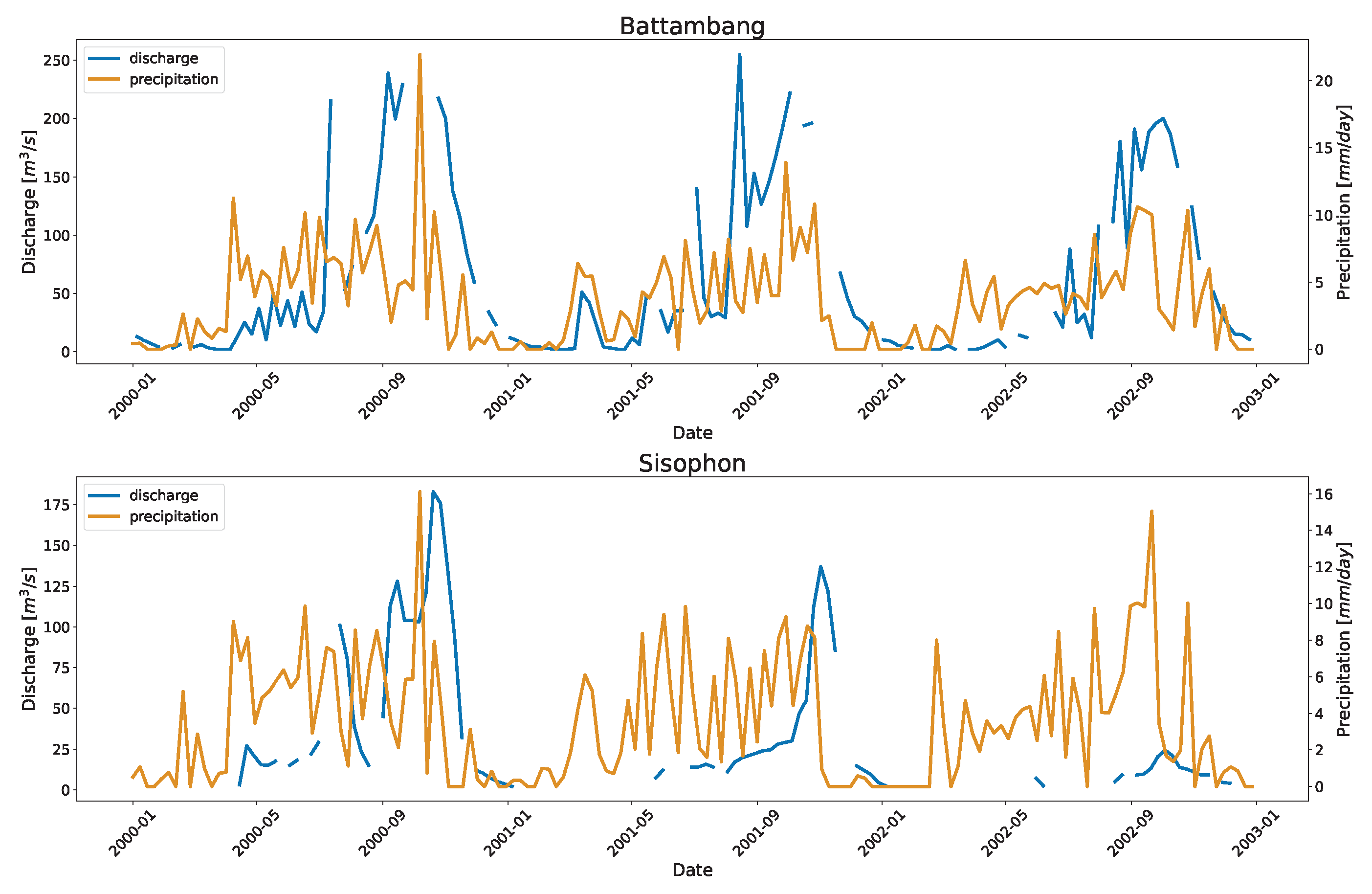
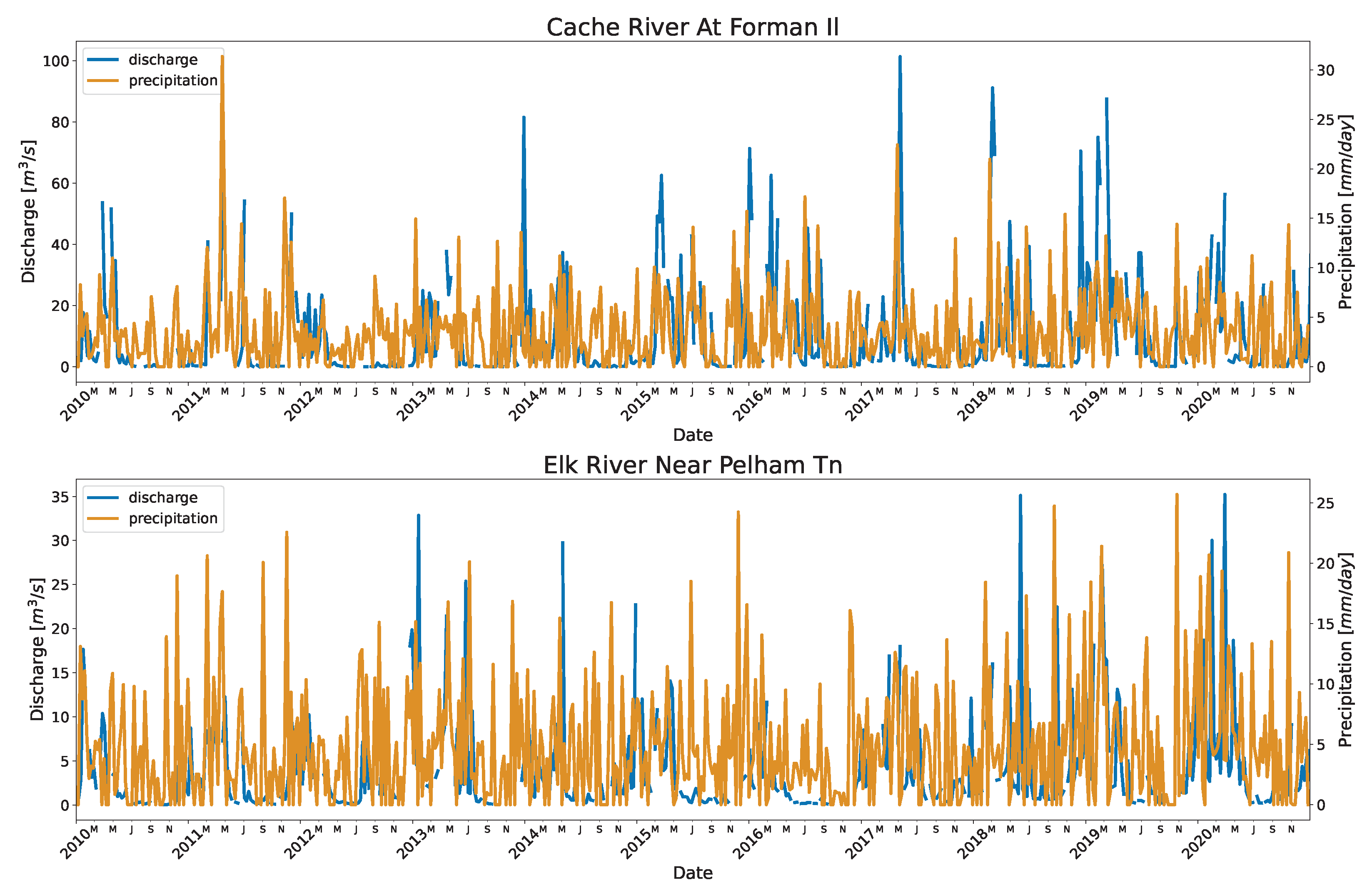
Other stations in Mekong, Battambang, and Sisophon also had high RRMSE with few data points on the high end. These stations lie on the tributaries outside the Mekong mainstream and contribute downstream to the Tonle Sap Lake. Seasonal rainfall may be linked to the increased flow during the wet season (Refer to
Figure A3) with a very low baseflow during the dry season. The other reason could be that those points were outliers not detected by the outlier algorithm. Similarly, stations in the US also have seasonal spike in their flow due to the rainfall events (Refer to
Figure A4)
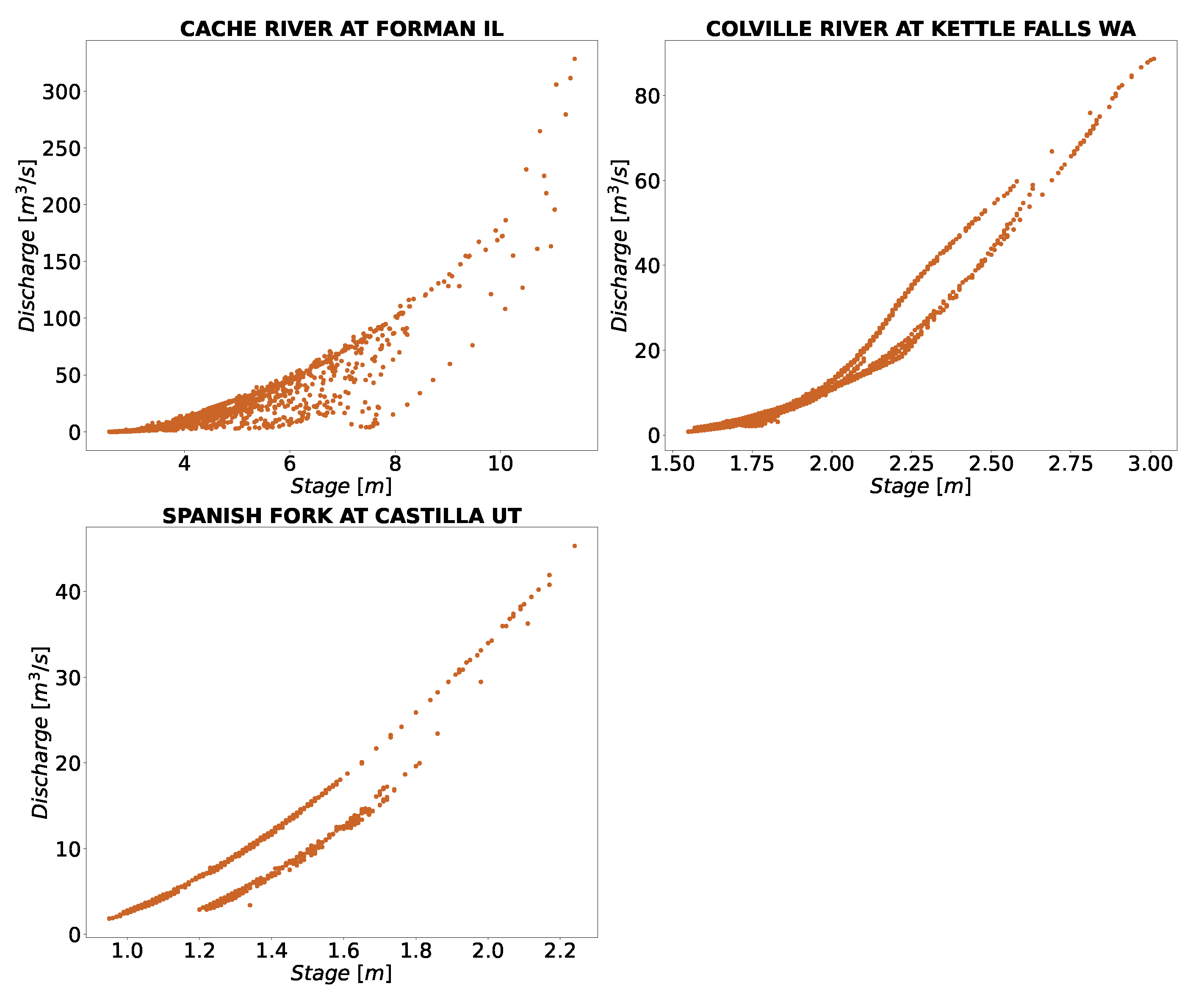
The rating curve tends to change over time; we noticed this phenomenon in several stations. The stations shown in
Figure 3 represent such conditions at stations in Cambodia, where different rating curve was observed. Some of the changes for the stations in the US are shown in
Figure 8. The runoff generating in Cambodia has a strong seasonality related to the wet season (June to November). Thus, separate rating curve may be explained by the rising and falling stage hydrograph. For stations considered here, depending upon dry or wet year, there could be up to two to three peaks with clear seasonality [
4,
65]. These are usually prevalent for high flow stations, like Stung Treng and Kratie. Thus, the clustering technique with the piecewise regression attempts to separate those rating curve and capture the non-linearity of the hydrograph.
One of the major opportunities (and a challenge) for the method was data quality in Cambodia. Significant data gaps or incomplete records were observed in many stations; in Neak Luong, the low flow was significantly different before 1971 compared to after the 1980s, with a data gap in between. Similarly, we observed that the model was mostly under predicting before the gap years (around 1970 or 1975) in Chaktomuk, Kompong Thom, and Kratie (
Figure A1). This may be linked to data quality or the inadequacy of the K-Means to separate them; other clustering algorithms based on density for example Density-Based Spatial Clustering of Applications with Noise DBSCAN [
66,
67] or based on distribution for example Gaussian Mixture Model [
68] may perform better.
We considered a second-order power stage-discharge relationship as this was found experimentally to fit most stations without being overly complicated in Cambodia. This relationship was consistent with the result [
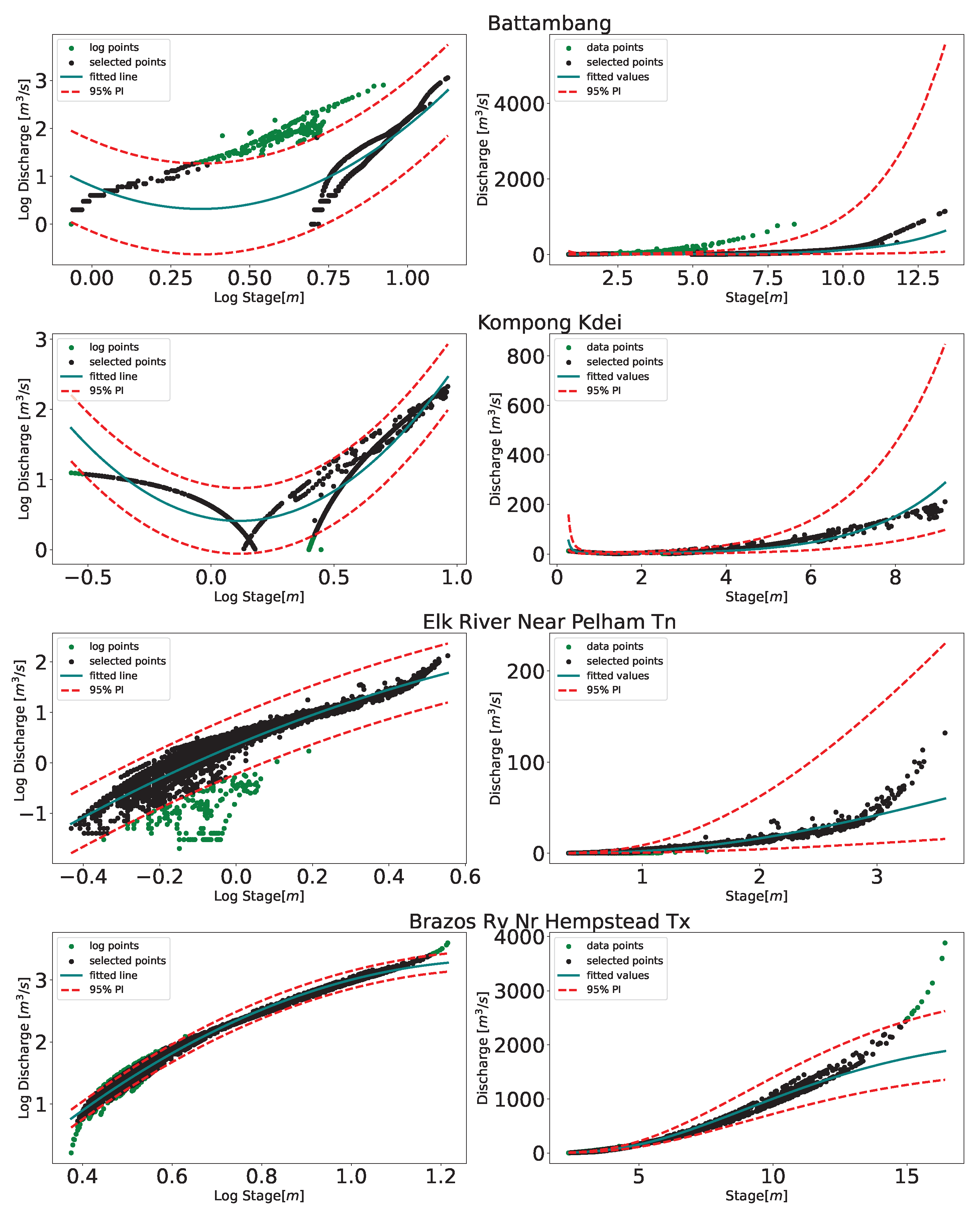
69] found in their study in the Mekong using the satellite altimetry stage data. With this relation, we then performed a 95% prediction interval. We noticed that, while this removed outliers from most of the stations and performed well, for some stations, e.g., Brazos River near Hempstead in Texas, as shown in
Figure 9, a higher-order relation may be desirable. In another study [
19], this station near Hempstead in Texas was also used. Even with the second-order relation removing some points in the high end (refer to
Figure 9), the maximum discharge was set at 2432.41 m
/s in this study as opposed to 1605 m
/s in [
19]; the NSE [
70] and RMSE of validation data-points (calculations not shown here) were 0.996 and 21.4 m
/s while it was 0.941 and 34.31 m
/s in [
19]. Thus, the longer time series gives higher probability of capturing the high-end or low-end events, which may be considered as a built-in extrapolation characteristics as compared to a traditional method where few data points are often used.
We tweaked several parameters that affected the model’s performance. These were determined experimentally. Some of them are:
- (1)
Threshold, controlling the absolute percent difference between the auto and percentile breakpoint, took numerical values.
- (2)
The Euclidean distance between the centers of the clusters: this parameter determined whether the cluster was necessary for the station and took numerical values.
- (3)
The outlier detection contained various parameters in the algorithm. For example, sklearn’s OneClassSVM, which was used in the study, has parameters like the upper bound on the fraction of training error (also called nu), choice of kernel, and kernel coefficient.
We determined a single set of parameters for the country. Adjusting individual station parameters may be desirable during an operational implementation of the method, which may further increase the confidence in the rating curve. Furthermore, we constrained our rating curve model to second-order polynomial fitting which may not represent the dynamics of the gauge height and discharge relationship in all cases. Additional constraints include assuming only one to two clusters for gauge height-discharge relationship where some stations may have three or more clusters. The rating curve results are only relevant within the data range of the training data used, extrapolating the rating curve outside the data range could lead to several uncertainties [
23,
71]. We did not test the error uncertainty for extrapolation, which should be used cautiously, although a time series based rating curve has higher probability of capturing the high-end and low-end events, as explained above, compared to traditional method where lesser data points are used. This study did not inspect the threshold for number of data points required to produce accuracy results (for the final results and at each step in the workflow), although investigation of how limited data influence the data driven results will be explored in future work. For this study the fewest number of data points to create the rating curve was 152 points at the Rio Tesuque Diversions station (
Figure 7). From a practical point of view, this method is useful for converting gauge height measurements to discharge, where there is relatively limited discharge data that is not measured regularly has not been updated.
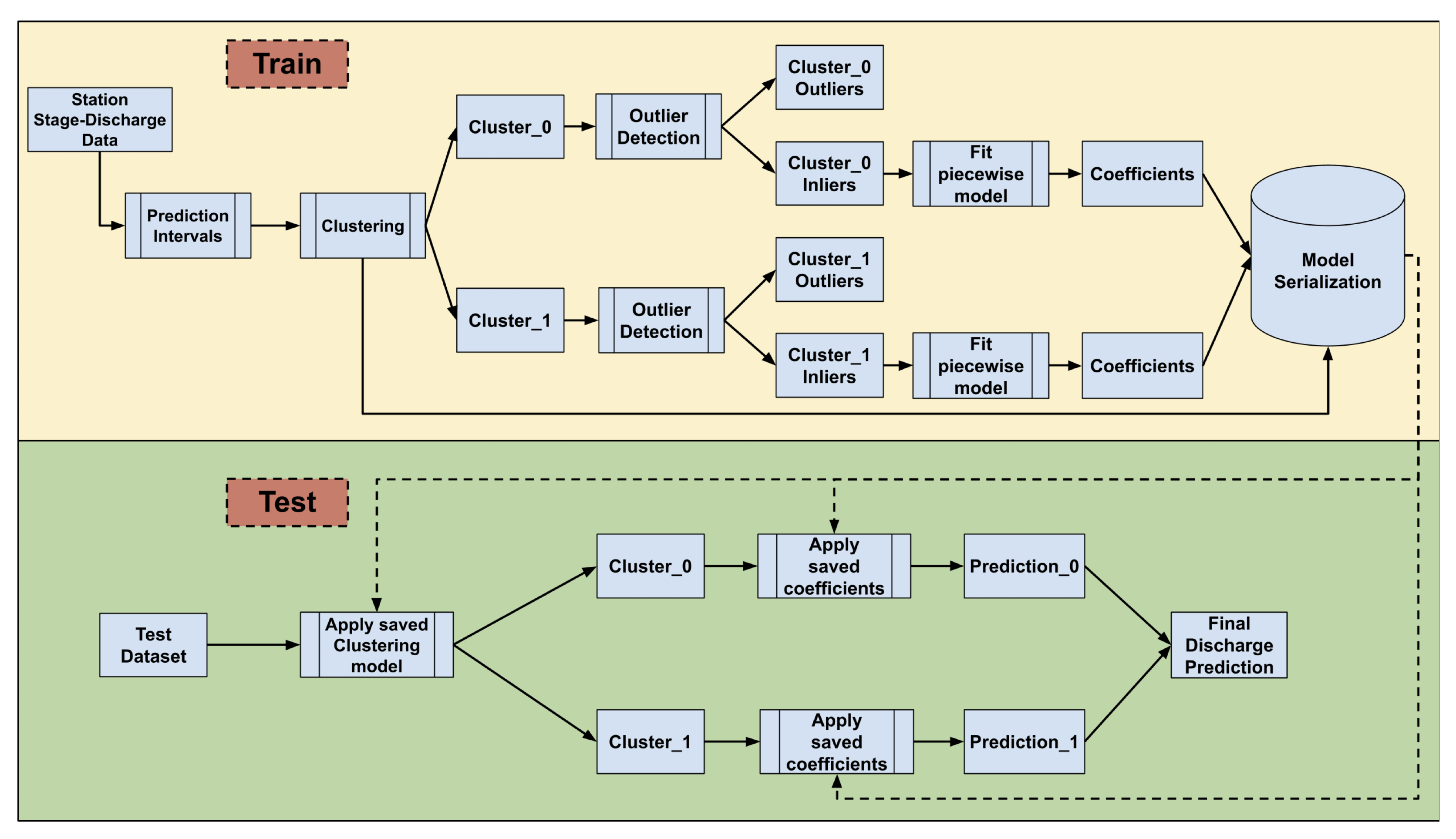
Data driven approaches typically obscure the decisions being made on data to produce the results [
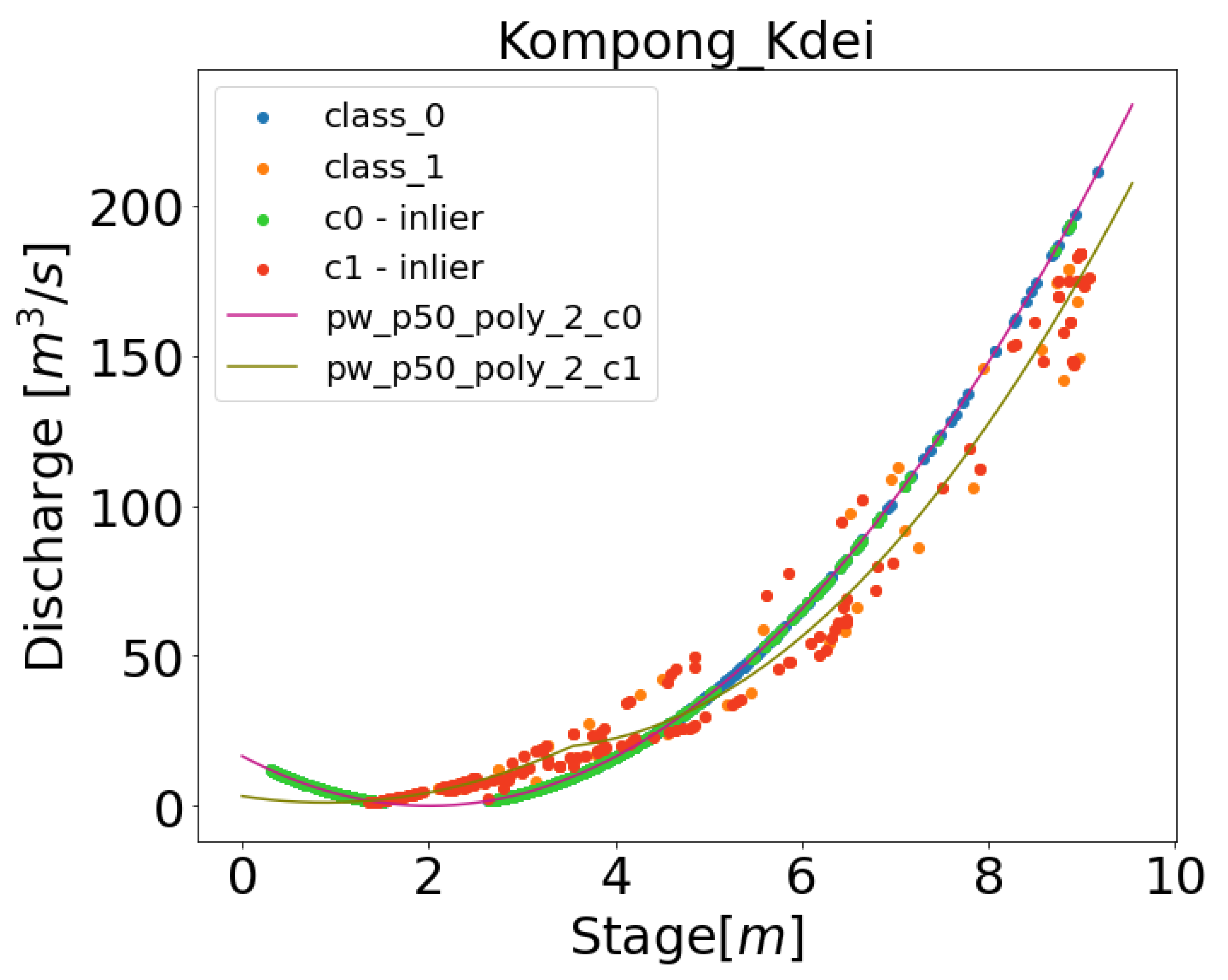
72]. Model interprebility for data driven approaches is important within the scientific disciplines as it lends to understanding of the models decisions and supports scientific discovery. The methodology presented in the paper combines multiple interpretable models including K-Means clustering, one-class SVM, and piece-wise polynomial regressions. As such, the different data driven decisions can be inspected and interrogated for additional information.
Figure 10 displays the results from multiple steps of training the DDRC for a station, in this case Kompong Kdei. It can be seen that the clustering determines the two best rating curves, while the outlier detection removes certain data points to refine a rating curve. Each individual component of these models can be output and interpreted to better understand how the data has informed the final rating curve result. Additional knowledge on particular flooding event to determine the breakpoints maybe integrated to increase the fitting accuracy of the rating curve. In addition to including physical attributes to drive the rating curve fitting, Physics Informed Neural Network (PINN) can be implemented in order to increase the robustness and interpretability of the model, for example, to incorporate information on backwater may also benefit. Future work will include investigating the application of PINNs for the rating curve fitting process.


 ,
, 