
Classification of Water Reservoirs in Terms of Ice Phenomena Using Advanced Statistical Methods—The Case of the Silesian Upland (Southern Poland)


Abstract
:1. Introduction
2. Materials and Methods
2.1. Studied Lakes
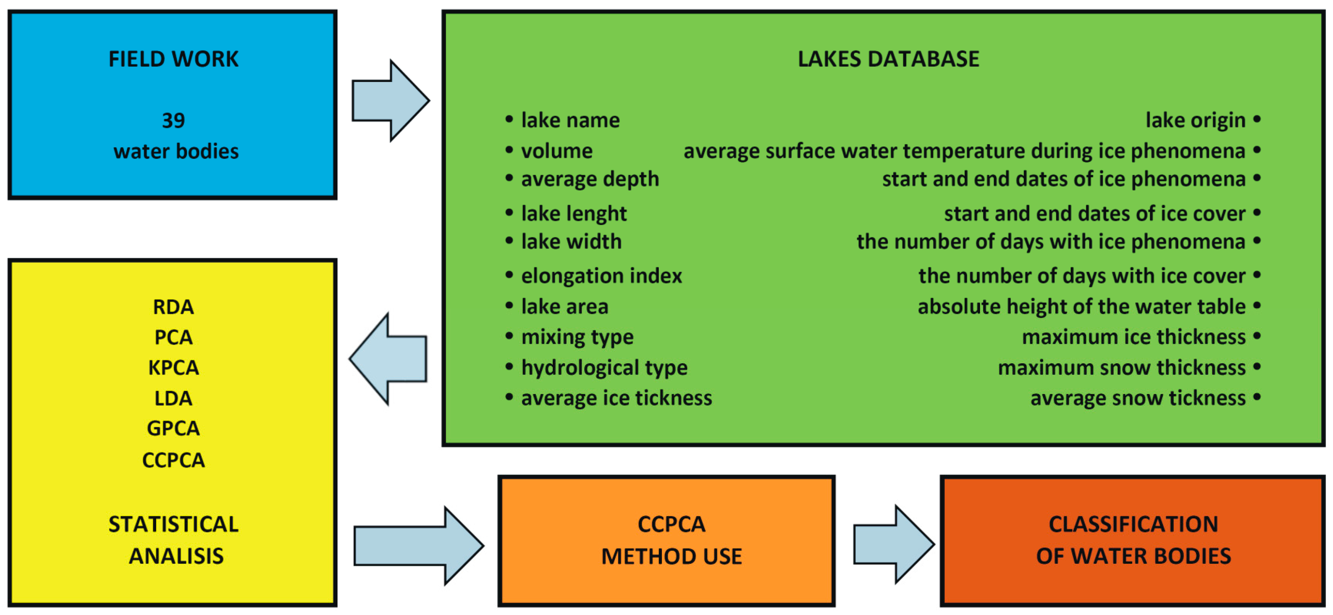
2.2. Field Work
2.3. Statistical Methods
- Determination of principal components using the CCPCA method; centroids are determined according to the cluster of traits and cases (traits are presented in columns and cases in rows);
- Use of different classifiers separately for each of the selected components. The goal is to check whether each case and feature will be correctly classified, i.e., assigned to a component; in this way, a number of clusters and classifier is determined such that they most accurately reflect the distribution of the feature and cases;
- Use of five-fold cross-validation to act against over-fitting to the data. This consists of dividing the collection randomly into five folds: four folds are used for teaching, and the last one is the fold used for testing. Then, the testing fold is attached to the teaching folds, and one of the teaching folds is the testing collection.
3. Results
4. Discussion
5. Conclusions
Author Contributions
Funding
Data Availability Statement
Acknowledgments
Conflicts of Interest
References
- Magnuson, J.J.; Robertson, D.M.; Benson, B.J.; Wynne, R.H.; Livingstone, D.M.; Arai, T.; Assel, R.A.; Barry, R.G.; Card, V.; Kuusisto, E.; et al. Historical trends in lake and river ice cover in the Northern Hemisphere. Science 2000, 289, 1743–1746. [Google Scholar] [CrossRef] [PubMed]
- Kirillin, G.; Leppäranta, M.; Terzhevik, A.; Granin, N.; Bernhardt, J.; Engelhardt, C.H.; Efremova, T.; Golosov, S.; Palshin, N.; Sherstyankin, P.; et al. Physics of seasonally ice-covered lakes: A review. Aquat. Sci. 2012, 74, 659–682. [Google Scholar] [CrossRef]
- Choiński, A.; Ptak, M.; Skowron, R.; Strzelczak, A. Changes in ice phenology on Polish lakes from 1961 to 2010 related to location and morphometry. Limnologica 2015, 53, 42–49. [Google Scholar] [CrossRef]
- Leppäranta, M. Freezing of Lakes and the Evolution of Their Ice Cover; Springer: Berlin/Heidelberg, Germany, 2015; pp. 1–301. [Google Scholar]
- Sharma, S.; Magnuson, J.J.; Batt, R.D.; Winslow, L.A.; Korhonen, J.; Aono, Y. Direct observations of ice seasonality reveal changes in climate over the past 320–570 years. Sci. Rep. 2016, 6, 25061. [Google Scholar] [CrossRef] [PubMed]
- Bartosiewicz, M.; Ptak, M.; Woolway, R.I.; Sojka, M. On thinning ice: Effects of atmospheric warming, changes in wind speed and rainfall on ice conditions in temperate lakes (Northern Poland). J. Hydrol. 2021, 597, 125724. [Google Scholar] [CrossRef]
- Piccolroaz, S.; Zhu, S.L.; Ptak, M.; Sojka, M.; Du, X.Z. Warming of lowland Polish lakes under future climate change scenarios and consequences for ice cover and mixing dynamics. J. Hydrol. Reg. Stud. 2021, 34, 100780. [Google Scholar] [CrossRef]
- Ptak, M.; Sojka, M. The disappearance of ice cover on temperate lakes (Central Europe) as a result of climate warming. Geogr. J. 2021, 187, 200–213. [Google Scholar] [CrossRef]
- Mishra, V.; Cherkauer, K.A.; Bowling, L.C.; Huber, M. Lake ice phenology of small lakes: Impacts of climate variability in the Great Lakes region. Glob. Planet. Chang. 2011, 76, 166–185. [Google Scholar] [CrossRef]
- Prowse, T.D.; Stephenson, R.L. The relationship between winter lake cover, radiation receipts and the oxygen deficit in temperate lakes. Atmos. Ocean 1986, 24, 386–403. [Google Scholar] [CrossRef]
- Fang, X.; Stefan, H.G. Potential climate warming effects on ice covers of small lakes in the contiguous U.S. Cold Reg. Sci. Technol. 1998, 27, 119–140. [Google Scholar] [CrossRef]
- Leppäranta, M.; Reinart, A.; Term, A.; Arst, H.; Hussainov, M.; Sipelgas, L. Investigation of ice and water properties and under-ice light fields in fresh and brackish water bodies. Nord. Hydrol. 2003, 34, 245–266. [Google Scholar] [CrossRef]
- Terzhevik, A.Y.; Pal’shin, N.I.; Golosov, S.D.; Zdorovennov, R.E.; Zdorovennova, G.E.; Mitrokhov, A.V.; Potakhin, M.S.; Shipunova, E.A.; Zverev, I.S. Hydrophysical aspects of oxygen regime formation in a shallow ice-covered lake. Water Resour. 2010, 37, 662–673. [Google Scholar] [CrossRef]
- Palecki, M.A.; Barry, R.G. Freeze-up and break-up of lakes as an index of temperature changes during the transition seasons: A case study for Finland. J. Appl. Meteorol. Climatol. 1986, 25, 893–902. [Google Scholar] [CrossRef]
- Livingstone, D.M. Ice break-up on southern Lake Baikal and its relationship to local and regional air temperatures in Siberia and to the North Atlantic Oscillation. Limnol. Oceanogr. 1999, 44, 1486–1497. [Google Scholar] [CrossRef]
- Hodgkins, G.A.; James II, I.C.; Huntington, T.G. Historical changes in lake ice-out dates as indicators of climate change in New England, 1850–2000. Int. J. Climatol. 2002, 22, 1819–1827. [Google Scholar] [CrossRef]
- Marszelewski, W.; Skowron, R. Ice cover as an indicator of winter air temperature changes: Case study of the Polish Lowland lakes. Hydrol. Sci. J. 2006, 51, 336–349. [Google Scholar] [CrossRef]
- Jensen, O.P.; Benson, B.J.; Magnuson, J.J.; Card, V.M.; Futter, M.N.; Soranno, P.A.; Stewart, K.M. Spatial analysis of ice phenology trends across the Laurentian Great Lakes region during a recent warming period. Limnol. Oceanogr. 2007, 52, 2013–2026. [Google Scholar] [CrossRef]
- Adrian, R.; O’Reilly, C.M.; Zagarese, H.; Baines, S.B.; Hessen, D.O.; Keller, W.; Livingstone, D.M.; Sommaruga, R.; Straile, D.; Van Donk, E.; et al. Lakes as sentinels of climate change. Limnol. Oceanogr. 2009, 54, 2283–2297. [Google Scholar] [CrossRef]
- Ghanbari, R.N.; Bravo, H.R.; Magnuson, J.J.; Hyzer, W.G.; Benson, B.J. Coherence between lake ice cover, local climate and teleconnections (Lake Mendota, Wisconsin). J. Hydrol. 2009, 374, 282–293. [Google Scholar] [CrossRef]
- Livingstone, D.M.; Adrian, R.; Blenckner, T.; George, G.; Weyhenmeyer, G.A. Lake ice phenology. In The Impact of Climate Change on European Lakes; George, G., Ed.; Aquatic Ecology Series 2010; Springer: Dordrecht, The Netherlands, 2010; Volume 4, pp. 51–62. [Google Scholar] [CrossRef]
- Karetnikov, S.; Naumenko, M. Lake Ladoga ice phenology: Mean condition and extremes during the last 65 years. Hydrol. Process. 2011, 25, 2859–2867. [Google Scholar] [CrossRef]
- Weyhenmeyer, G.A.; Livingstone, D.M.; Meili, M.; Jensen, O.; Benson, B.; Magnuson, J.J. Large geographical differences in the sensitivity of ice-covered lakes and rivers in the Northern Hemisphere to temperature changes. Glob. Chang. Biol. 2011, 17, 268–275. [Google Scholar] [CrossRef]
- Benson, B.J.; Magnuson, J.J.; Jensen, O.P.; Card, V.M.; Hodgkins, G.; Korhonen, J.; Livingstone, D.M.; Stewart, K.M.; Weyhenmeyer, G.A.; Granin, N.G. Extreme events, trends, and variability in Northern Hemisphere lake-ice phenology (1855–2005). Clim. Chang. 2012, 112, 299–323. [Google Scholar] [CrossRef]
- Mudelsee, M.A. Proxy record of winter temperatures since 1836 from ice freeze-up/breakup in lake Näsijärvi, Finland. Clim. Dyn. 2012, 38, 1413–1420. [Google Scholar] [CrossRef]
- Sharma, S.; Blagrave, K.; Magnuson, J.J.; O’Reilly, C.M.; Oliver, S.; Batt, R.D.; Magee, M.R.; Straile, D.; Weyhenmeyer, G.A.; Winslow, L.; et al. Widespread loss of lake ice around the Northern Hemisphere in a warming world. Nat. Clim. Chang. 2019, 9, 227–231. [Google Scholar] [CrossRef]
- Solarski, M.; Rzetala, M. Ice Regime of the Kozłowa Góra Reservoir (Southern Poland) as an Indicator of Changes of the Thermal Conditions of Ambient Air. Water 2020, 12, 2435. [Google Scholar] [CrossRef]
- Bengtsson, L. Spatial variability of lake ice covers. Geogr. Annaler. Ser. A Phys. Geogr. 1986, 68, 113–121. [Google Scholar] [CrossRef]
- Champlin, J.G.; Stefan, H.G. Field Study of the Ice Cover of a Lake: Implications for Winter Water Quality Modeling; Project Report No. 387; St. Anthony Falls Laboratory, University of Minnesota: Minneapolis, MN, USA, 1996; pp. 1–212. [Google Scholar]
- Launiainen, J.; Cheng, B. Modelling of ice thermodynamics in natural water bodies. Cold Reg. Sci. Technol. 1998, 27, 153–178. [Google Scholar] [CrossRef]
- Aihara, M.; Chikita, K.A.; Momoki, Y.; Mabuchi, S. A physical study on the thermal ice ridge in a closed deep lake: Lake Kuttara, Hokkaido, Japan. Limnology 2010, 11, 125–132. [Google Scholar] [CrossRef]
- Solarski, M.; Pradela, A.; Rzetala, M. Natural and anthropogenic influences on ice formation on various water bodies of the Silesian Upland (southern Poland). Limnol. Rev. 2011, 11, 33–44. [Google Scholar] [CrossRef]
- Choiński, A.; Ptak, M. Variation in the ice cover thickness on Lake Samołęskie as a result of underground water supply. Limnol. Rev. 2012, 12, 33–138. [Google Scholar] [CrossRef]
- Machowski, R. Course of ice phenomena in small water reservoir in Katowice (Poland) in the winter season 2011/2012. Environ. Socio-Econ. Stud. 2013, 1, 7–13. [Google Scholar] [CrossRef]
- Solarski, M. The ice phenomena dynamics of small anthropogenic water bodies in the Silesian Upland, Poland. Environ. Socio-Econ. Stud. 2017, 5, 74–81. [Google Scholar] [CrossRef]
- Solarski, M.; Szumny, M. Conditions of spatiotemporal variability of the thickness of the ice cover on lakes in the Tatra Mountains. J. Moutain Sci. 2020, 17, 2369–2386. [Google Scholar] [CrossRef]
- Solarski, M.; Rzetala, M. Changes in the Thickness of Ice Cover on Water Bodies Subject to Human Pressure (Silesian Upland, Southern Poland). Front. Earth Sci. 2021, 9, 675216. [Google Scholar] [CrossRef]
- Solarski, M.; Rzetala, M. Determinants of Spatial Variability of Ice Thickness in Lakes in High Mountains of the Temperate Zone—The Case of the Tatra Mountains. Water 2022, 14, 2360. [Google Scholar] [CrossRef]
- Assel, R.A.; Cronk, K.; Norton, D. Recent Trends in Laurentian Great Lakes ice cover. Clim. Chang. 2003, 57, 185–204. [Google Scholar] [CrossRef]
- Williams, G.; Layman, K.L.; Stefan, H.G. Dependence of lake ice on climate, geographic and bathymetric variables. Cold Reg. Sci. Technol. 2004, 40, 145–164. [Google Scholar] [CrossRef]
- Wang, J.; Bai, X.; Hu, H.; Clites, A.; Colton, M.; Lofgren, B. Temporal and spatial variability of Great Lakes ice cover, 1973–2010. J. Clim. 2012, 25, 1318–1329. [Google Scholar] [CrossRef]
- Engram, M.; Arp, C.D.; Jones, B.M.; Ajadi, O.A.; Meyer, F.J. Analyzing floating and bedfast lake ice regimes across Arctic Alaska using 25 years of space-borne SAR imagery. Remote Sens. Environ. 2018, 209, 660–676. [Google Scholar] [CrossRef]
- Gądek, B.; Szumny, M.; Szypula, B. Classification of the Tatra Mountain lakes in terms of the duration of their ice cover (Poland and Slovakia). J. Limnol. 2020, 79, 70–81. [Google Scholar] [CrossRef]
- Ptak, M.; Sojka, M.; Nowak, B. Changes in Ice Regime of Jagodne Lake (North-Eastern Poland). Acta Sci. Pol. Form. Circumiectus 2019, 18, 89–100. [Google Scholar] [CrossRef]
- Kantor-Pietraga, I.; Krzysztofik, R.; Solarski, M. Planning Recreation around Water Bodies in Two Hard Coal Post-Mining Areas in Southern Poland. Sustainability 2023, 15, 10607. [Google Scholar] [CrossRef]
- Rzetala, M.; Jagus, A. New lake district in Europe: Origin and hydrochemical characteristics. Water Environ. J. 2012, 26, 108–117. [Google Scholar] [CrossRef]
- Ringnér, M. What is principal component analysis? Nat. Biotechnol. 2008, 26, 303–304. [Google Scholar] [CrossRef] [PubMed]
- Schölkopf, B. The kernel trick for distances. In Advances in Neural Information Processing Systems; Leen, T.K., Dietterich, T.G., Tresp, V., Eds.; MIT Press: Cambridge, MA, USA, 2001; pp. 301–307. [Google Scholar]
- Leśkiewicz, M.; Kaliszewski, M.; Mierczyk, Z.; Włodarski, M. Comparison of principal component analysis and linear discriminant analysis applied to classification of excitation-emission matrices of the selected biological material. Biul. Wojsk. Akad. Tech. 2016, 65, 15–31. [Google Scholar] [CrossRef]
- Topolski, M. Algorithm of multidimensional analysis of main features of PCA with blurry observation of facility features detection of carcinoma cells multiple myeloma. In Proceedings of the 11th International Conference on Computer Recognition Systems, Polanica Zdroj, Poland, 20–22 May 2019; Springer: Cham, Switzerland, 2019; pp. 286–294. [Google Scholar]
- Topolski, M. The Modified Principal Component Analysis Feature Extraction Method for the Task of Diagnosing Chronic Lymphocytic Leukemia Type B-CLL. J. Univers. Comput. Sci. 2020, 26, 734–746. [Google Scholar] [CrossRef]
- Topolski, M.; Topolska, K. Algorithm for Constructing a Classifier Team Using a Modified PCA (Principal Component Analysis) in the Task of Diagnosis of Acute Lymphocytic Leukaemia Type B-CLL. In Hybrid Artificial Intelligent Systems, Proceedings of the 14th International Conference, HAIS 2019, León, Spain, 4–6 September 2019; Lecture Notes in Computer Science; Pérez García, H., Sánchez González, L., Castejón Limas, M., Quintián Pardo, H., Corchado Rodríguez, E., Eds.; Springer: Cham, Switzerland, 2019; Volume 11734, pp. 614–624. [Google Scholar] [CrossRef]
- Topolski, M. Application of the Stochastic Gradient Method in the Construction of the Main Components of PCA in the Task Diagnosis of Multiple Sclerosis in Children. In Computational Science, Proceedings of the 20th International Conference on Computational Science, ICCS 2020, Amsterdam, The Netherlands, 3–5 June 2020; Lecture Notes in Computer Science; Springer: Cham, Switzerland, 2020; Volume 12140, pp. 35–44. [Google Scholar] [CrossRef]
- Leppäranta, M. Modelling the formation and decay of lake ice. In The Impact of Climate Change on European Lakes; George, G., Ed.; Springer: Dordrecht, The Netherlands, 2009; pp. 63–83. [Google Scholar]
- Richards, T.O. The meteorological aspects of ice cover on the Great Lakes. Mon. Weather Rev. 1964, 92, 297–302. [Google Scholar] [CrossRef]
- Vavrus, S.J.; Wynne, R.H.; Foley, J.A. Measuring the sensitivity of southern Wisconsin lake ice to climate variations and lake depth using a numerical model. Limnol. Oceanogr. 1996, 41, 822–831. [Google Scholar] [CrossRef]
- Gao, S.B.; Stefan, H.G. Multiple linear regression for lake ice and lake temperature characteristics. J. Cold Reg. Eng. 1999, 13, 59–77. [Google Scholar] [CrossRef]
- Ménard, P.; Duguay, C.R.; Flato, G.M.; Rouse, W.R. Simulation of ice phenology on Great Slave Lake, Northwest Territories, Canada. Hydrol. Process. 2002, 16, 3691–3706. [Google Scholar] [CrossRef]
- Futter, M.N. Patterns and trends in Southern Ontario Lake ice phenology. Environ. Monit. Assess. 2003, 88, 431–444. [Google Scholar] [CrossRef] [PubMed]
- Bernhardt, J.; Engelhardt, C.; Kirillin, G.; Matschullat, J. Lake ice phenology in Berlin-Brandenburg from 1947–2007: Observations and model hindcasts. Clim. Chang. 2012, 112, 791–817. [Google Scholar] [CrossRef]
- Solarski, M.; Rzetala, M. A Comparison of Model Calculations of Ice Thickness with the Observations on Small Water Bodies in Katowice Upland (Southern Poland). Water 2022, 14, 3886. [Google Scholar] [CrossRef]


| No. | Lake | Origin (1) | Volume | Average Depth | Lake Length | Lake Width | Elongation Index | Absolute Height of the Water Table | Lake Area | Mixing Type (2) | Hydrological Type (3) |
|---|---|---|---|---|---|---|---|---|---|---|---|
| [m3·103] | [m] | [km] | [km] | [m a.s.l.] | [ha] | ||||||
| 1 | Akwen | Pe | 62.3 | 2.6 | 0.2 | 0.1 | 0.9 | 241.0 | 2.4 | P | B |
| 2 | Amendy | Pe | 21.4 | 1.6 | 0.1 | 0.1 | 0.8 | 287.7 | 1.3 | P | B |
| 3 | Balaton | Pe | 68.8 | 0.9 | 0.4 | 0.3 | 8.2 | 262.0 | 7.4 | P | O |
| 4 | Brantka | N | 625.7 | 2.9 | 1.0 | 0.5 | 7.3 | 270.0 | 21.3 | P | O |
| 5 | Brzeziny | S | 9.6 | 1.1 | 0.2 | 0.1 | 0.8 | 283.1 | 0.9 | P | O |
| 6 | Dzierżno Duże | Pe | 66,000.0 | 11.2 | 5.7 | 1.5 | 52.4 | 199.0 | 587.2 | D | P |
| 7 | Farskie | N | 149.5 | 1.2 | 0.6 | 0.3 | 10.3 | 212.0 | 12.3 | P | P |
| 8 | Gliniok | N | 37.0 | 1.7 | 0.2 | 0.2 | 1.3 | 288.2 | 2.2 | P | O |
| 9 | Grunfeld | Pe | 179.0 | 4.6 | 0.3 | 0.2 | 0.8 | 290.0 | 3.9 | P | B |
| 10 | Hubertus II | Pe | 249.4 | 1.4 | 0.9 | 0.2 | 13.0 | 248.0 | 18.2 | P | O |
| 11 | Kajakowy | Pg | 244.4 | 2.4 | 0.6 | 0.2 | 4.2 | 258.8 | 10.0 | P | P |
| 12 | Kamieniec | G | 25.1 | 0.8 | 0.3 | 0.1 | 4.0 | 233.1 | 3.2 | P | P |
| 13 | Kozłowa Góra | Z | 13,050.0 | 3.0 | 3.4 | 1.8 | 144.0 | 278.6 | 432.0 | P | P |
| 14 | Kuźnica Warężyńska | Pe | 51,100.0 | 9.4 | 5.2 | 1.7 | 57.9 | 264.0 | 543.8 | D | P |
| 15 | Leśny | N | 1011.5 | 3.0 | 0.9 | 0.6 | 11.1 | 240.0 | 33.4 | P | O |
| 16 | Łąka | Pg | 292.0 | 2.2 | 0.8 | 0.3 | 6.0 | 258.5 | 13.1 | P | P |
| 17 | Maroko | Pg | 109.5 | 1.4 | 0.6 | 0.2 | 5.8 | 264.9 | 8.1 | P | B |
| 18 | Moczury | N | 231.2 | 1.6 | 0.6 | 0.3 | 9.1 | 244.5 | 14.5 | P | O |
| 19 | Morawa | Pe | 559.1 | 1.6 | 0.8 | 0.6 | 21.7 | 250.1 | 34.7 | P | O |
| 20 | Nakło-Chechło | Pe | 2100.0 | 2.6 | 2.1 | 0.8 | 30.8 | 289.3 | 80.1 | P | O |
| 21 | Niezdara N | Pg | 0.4 | 0.2 | 0.2 | 0.0 | 1.0 | 278.0 | 0.2 | P | P |
| 22 | Niezdara S | Pg | 0.2 | 0.2 | 0.0 | 0.0 | 0.5 | 278.5 | 0.1 | P | B |
| 23 | Ostrożnica | G | 21.5 | 0.5 | 0.5 | 0.2 | 8.2 | 280.5 | 4.1 | P | P |
| 24 | Pod Borem | S | 72.2 | 3.8 | 0.2 | 0.1 | 0.5 | 282.0 | 1.9 | A | P |
| 25 | Pogoria III | Pe | 12,000.0 | 5.7 | 2.0 | 1.7 | 37.1 | 261.5 | 211.2 | D | P |
| 26 | Przetok | Pe | 16.8 | 1.1 | 0.3 | 0.1 | 1.4 | 260.0 | 1.5 | P | O |
| 27 | Rogoźnik Duży | Pe | 272.9 | 1.2 | 1.6 | 0.2 | 19.8 | 291.9 | 23.7 | P | P |
| 28 | Rozlewisko Bytomki | N | 14.3 | 1.2 | 0.2 | 0.1 | 1.0 | 243.0 | 1.2 | P | B |
| 29 | Skałka | S | 110.3 | 1.9 | 0.3 | 0.3 | 3.1 | 276.1 | 5.9 | P | B |
| 30 | Smrodlok | N | 46.4 | 1.6 | 0.3 | 0.2 | 1.8 | 284.5 | 2.9 | P | B |
| 31 | Somerek | S | 131.1 | 3.1 | 0.3 | 0.2 | 1.4 | 266.2 | 4.2 | A | P |
| 32 | Sośnica-Makoszowy | S | 189.0 | 4.5 | 0.3 | 0.2 | 0.9 | 224.0 | 4.2 | A | P |
| 33 | Szczygłowice | N | 471.2 | 2.2 | 0.6 | 0.5 | 9.5 | 228.0 | 21.0 | P | O |
| 34 | Szkopka | Pg | 21.8 | 1.6 | 0.3 | 0.1 | 0.9 | 245.2 | 1.4 | P | B |
| 35 | Trupek | Pe | 8.1 | 1.2 | 0.1 | 0.1 | 0.6 | 288.0 | 0.7 | P | B |
| 36 | Trzy Stawy M. | G | 2.7 | 0.9 | 0.1 | 0.1 | 0.3 | 285.2 | 0.3 | P | P |
| 37 | Przy Leśnej | N | 2.0 | 0.7 | 0.1 | 0.1 | 0.4 | 259.4 | 0.3 | P | B |
| 38 | Żabie Doły N | Pg | 140.4 | 1.5 | 0.6 | 0.3 | 6.3 | 277.1 | 9.4 | P | O |
| 39 | Żabie Doły S | N | 43.3 | 1.7 | 0.2 | 0.1 | 1.5 | 278.0 | 2.6 | P | B |
| No. of Water Bodies(See Table 1) | Start and End Dates of Ice Phenomena | Start and End Dates of Ice Cover | Average Surface Water Temperature during Ice Phenomena | Maximum Ice Thickness (Maximum Snow Ice Thickness) | Average Ice Thickness | Average Snow Thickness | The Number of days with Ice Phenomena | The Number of Days with Ice Cover |
|---|---|---|---|---|---|---|---|---|
| (°C) | (cm) | (Number of Days) | ||||||
| 1 | 13 December–24 March | 17 December–16 March | 1.2 | 27.0 (9.0) | 16.3 | 7.8 | 101 | 93 |
| 2 | 13 December–22 March | 18 December–16 March | 1.9 | 22.5 (11.0) | 13.2 | 6.3 | 99 | 94 |
| 3 | 13 December–24 March | 16 December–15 March | 2.1 | 22.5 (14.0) | 11.6 | 4.3 | 101 | 94 |
| 4 | 13 December–24 March | 18 December–06 February | 1.9 | 26.0 (13.0) | 15.0 | 5.3 | 101 | 96 |
| 5 | 13 December–24 March | 15 December–15 March | 0.6 | 23.0 (15.0) | 12.8 | 8.1 | 101 | 95 |
| 6 | 05 January–13 March | 11 January–25 February | 2.4 | 22.0 (8.0) | 13.0 | 6.4 | 67 | 53 |
| 7 | 13 December–16 March | 19 November–22 December | 2.5 | 27.0 (8.0) | 12.2 | 4.0 | 93 | 73 |
| 8 | 14 December–24 March | 15 December–17 March | 1.7 | 25.5 (15.0) | 14.1 | 6.4 | 101 | 97 |
| 9 | 15 December–24 March | 19 December–17 March | 1.4 | 25.0 (15.0) | 15.1 | 4.7 | 99 | 93 |
| 10 | 14 December–23 March | 18 December–15 March | 2.2 | 22.5 (9.0) | 14.3 | 4.5 | 99 | 92 |
| 11 | 16 December–22 March | 19 December–15 March | 2.0 | 26.0 (16.0) | 14.6 | 5.5 | 96 | 90 |
| 12 | 13 December–22 March | 15 December–13 March | 2.6 | 21.0 (11.0) | 12.5 | 5.6 | 99 | 94 |
| 13 | 14 December–23 March | 18 December–18 March | 1.5 | 29.0 (15.0) | 19.1 | 7.2 | 99 | 93 |
| 14 | 17 December–26 March | 2 January–19 March | 1.6 | 29.5 (12.0) | 19.2 | 4.6 | 99 | 92 |
| 15 | 14 December–23 March | 19 December–13 March | 1.8 | 28.5 (10.0) | 15.3 | 5.3 | 99 | 93 |
| 16 | 16 December–22 March | 25 January–9 February | 1.7 | 26.0 (10.0) | 14.7 | 5.6 | 96 | 89 |
| 17 | 13 December–24 March | 17 December–27 January | 1.1 | 28.0 (10.0) | 13.5 | 5.8 | 101 | 94 |
| 18 | 14 December–21 March | 18 December–27 January | 1.7 | 26.0 (10.0) | 11.7 | 6.4 | 97 | 91 |
| 19 | 14 December–23 March | 20 January–17 March | 2.0 | 28.0 (10.0) | 14.4 | 4.5 | 99 | 93 |
| 20 | 13 December–24 March | 18 December–17 March | 2.3 | 26.0 (10.0) | 16.0 | 6.7 | 101 | 94 |
| 21 | 13 December–17 March | 14 December–22 December | 3.9 | 13.0 (7.0) | 4.4 | 1.4 | 85 | 58 |
| 22 | 13 December–24 March | 14 December–16 March | 2.0 | 22.0 (12.0) | 13.7 | 5.5 | 102 | 97 |
| 23 | 13 December–27 March | 17 December–16 March | 1.7 | 29.5 (15.0) | 18.4 | 7.9 | 104 | 99 |
| 24 | (-) | (-) | 12.6 | (-) | (-) | (-) | 0 | 0 |
| 25 | 17 December–26 March | 2 January–16 March | 1.8 | 25.0 (10.0) | 16.9 | 4.6 | 99 | 93 |
| 26 | 13 December–23 March | 2 January–19 February | 1.0 | 26.0 (14.0) | 16.3 | 5.6 | 100 | 97 |
| 27 | 13 December–25 March | 17 December–16 March | 1.5 | 27.5 (10.0) | 15.7 | 7.3 | 102 | 97 |
| 28 | 13 December–23 March | 16 December–15 March | 1.4 | 19.0 (11.0) | 12.0 | 5.3 | 100 | 96 |
| 29 | 14 December–21 March | 16 December–14 March | 1.8 | 24.0 (8.0) | 13.4 | 5.8 | 97 | 94 |
| 30 | 13 December–25 March | 16 December–17 March | 1.6 | 26.0 (13.0) | 17.8 | 6.8 | 102 | 96 |
| 31 | 24 January–07 February | (-) | 7.9 | 2.0 (-) | 1.1 | 0.5 | 14 | 2 |
| 32 | 23 January–01 February | (-) | 9.0 | 1.0 (-) | 0.4 | (-) | 9 | 0 |
| 33 | 13 December–22 March | 17 December–15 March | 1.6 | 23.0 (11.0) | 13.4 | 5.3 | 99 | 93 |
| 34 | 13 December–26 March | 15 December–17 March | 1.8 | 26.0 (12.0) | 16.8 | 4.1 | 103 | 100 |
| 35 | 13 December–24 March | 13 December–17 March | 1.8 | 27.0 (14.0) | 16.8 | 6.7 | 100 | 100 |
| 36 | 13 December–22 March | 14 December–13 March | 2.5 | 24.0 (13.0) | 12.6 | 5.4 | 97 | 97 |
| 37 | 13 December–21 March | 13 December–17 March | 1.0 | 26.0 (12.0) | 16.4 | 6.5 | 96 | 96 |
| 38 | 14 December–21 March | 16 December–17 March | 2.3 | 21.0 (11.0) | 12.6 | 5.9 | 94 | 94 |
| 39 | 13 December–21 March | 18 December–17 March | 1.9 | 23.0 (12.0) | 14.0 | 5.1 | 94 | 94 |
| No. of Water Bodies (See Table 1) | start and End Dates of Ice Phenomena | Start and End Dates of Ice Cover | Average Surface Water Temperature during Ice Phenomena | Maximum Ice Thickness (Maximum Snow Ice Thickness) | Average Ice Thickness | Average Snow Thickness | The Number of Days with Ice Phenomena | The Number of Days with Ice Cover |
|---|---|---|---|---|---|---|---|---|
| (°C) | (cm) | (Number of Days) | ||||||
| 1 | 27 November – 20 March | 23 January–10 March | 1.1 | 22.0 (10.0) | 15.2 | 3.8 | 113 | 103 |
| 2 | 27 November–15 March | 1 December–9 March | 0.8 | 21.0 (11.0) | 14.3 | 3.8 | 108 | 102 |
| 3 | 26 November–17 March | 30 November–9 March | 1.6 | 18.5 (10.0) | 11.1 | 3.8 | 111 | 103 |
| 4 | 28 November–17 March | 4 December–9 March | 0.7 | 22.0 (9.0) | 15.2 | 4.8 | 109 | 104 |
| 5 | 26 November–20 March | 29 November–9 March | 1.4 | 20.0 (13.0) | 15.6 | 3.8 | 114 | 108 |
| 6 | 16 December–14 March | 21 December–9 March | 1.9 | 17.0 (4.0) | 8.4 | 0.9 | 86 | 70 |
| 7 | 27 November–16 March | 28 December–9 March | 1.3 | 18.0 (12.0) | 9.7 | 3.5 | 109 | 92 |
| 8 | 28 November–17 March | 30 November–9 March | 1.0 | 21.5 (13.0) | 15.5 | 4.5 | 109 | 106 |
| 9 | 2 December–18 March | 5 December–9 March | 1.2 | 19.0 (12.0) | 13.7 | 3.1 | 106 | 102 |
| 10 | 28 November–16 March | 5 December–9 March | 1.3 | 21.5 (15.0) | 14.3 | 2.6 | 108 | 101 |
| 11 | 28 November–16 March | 3 December–9 March | 1.1 | 22.5 (15.0) | 16.3 | 2.7 | 108 | 103 |
| 12 | 27 November–14 March | 30 November–08 March | 1.4 | 16.0 (8.0) | 11.3 | 3.6 | 107 | 100 |
| 13 | 26 November–19 March | 4 December–13 March | 0.8 | 25.0 (13.0) | 16.9 | 2.9 | 113 | 103 |
| 14 | 3 December–18 March | 17 December–9 March | 1.3 | 19.0 (5.0) | 12.9 | 1.9 | 105 | 91 |
| 15 | 2 December– 16 March | 5 December–9 March | 1.1 | 21.0 (10.0) | 12.6 | 3.0 | 104 | 99 |
| 16 | 29 November–16 March | 2 December–9 March | 1.4 | 18.5 (12.0) | 12.8 | 3.2 | 107 | 100 |
| 17 | 28 November–19 March | 1 December–9 March | 0.8 | 19.0 (13.0) | 14.6 | 3.6 | 111 | 104 |
| 18 | 27 November–15 March | 4 December– 9 March | 0.8 | 21.5 (13.0) | 14.3 | 4.0 | 108 | 102 |
| 19 | 27 November–16 March | 5 December–9 March | 1.2 | 21.5 (14.0) | 15.0 | 3.6 | 109 | 99 |
| 20 | 28 November–16 March | 3 December–9 March | 1.0 | 20.0 (12.0) | 15.4 | 2.8 | 108 | 100 |
| 21 | 26 November–11 March | 2 December–5 March | 3.0 | 14.0 (2.0) | 5.3 | 2.0 | 87 | 59 |
| 22 | 26 November–19 March | 26 November–9 March | 0.8 | 21.5 (12.0) | 14.0 | 2.9 | 113 | 109 |
| 23 | 26 November–20 March | 26 November–11 March | 0.5 | 26.0 (14.0) | 18.7 | 4.4 | 114 | 112 |
| 24 | (-) | (-) | 12.9 | (-) | (-) | (-) | 0 | 0 |
| 25 | 5 December–19 March | 19 December–10 March | 1.1 | 22.5 (2.0) | 14.7 | 1.6 | 104 | 92 |
| 26 | 26 November–18 March | 1 December–9 March | 1.0 | 20.0 (9.0) | 14.6 | 5.0 | 112 | 107 |
| 27 | 29 November– 18 March | 30 November–9 March | 1.1 | 23.5 (10.0) | 17.6 | 4.1 | 109 | 105 |
| 28 | 26 November–17 March | 29 November–08 March | 0.6 | 21.0 (10.0) | 16.2 | 3.5 | 111 | 106 |
| 29 | 28 November–15 March | 2 December–9 March | 1.0 | 21.0 (9.0) | 15.1 | 4.6 | 107 | 102 |
| 30 | 27 November–19 March | 1 December–9 March | 0.8 | 22.0 (7.0) | 15.8 | 4.1 | 112 | 104 |
| 31 | 29 December–31 December | (-) | 7.7 | 0.5 (0.0) | (-) | (-) | 3 | 0 |
| 32 | 30 November–25 February | (-) | 5.2 | 1.0 (0.0) | 0.1 | 0.0 | 13 | 0 |
| 33 | 27 November–16 March | 5 December–9 March | 1.6 | 21.5 (10.0) | 12.4 | 3.1 | 109 | 99 |
| 34 | 26 November–20 March | 30 November–11 March | 0.9 | 24.0 (11.0) | 16.0 | 3.5 | 114 | 107 |
| 35 | 26 November–19 March | 30 November–9 March | 0.9 | 26.0 (12.0) | 17.9 | 4.7 | 113 | 107 |
| 36 | 26 November–17 March | 4 December–9 March | 1.2 | 14.0 (11.0) | 9.0 | 3.7 | 111 | 106 |
| 37 | 26 November–17 March | 27 November–9 March | 1.5 | 21.5 (16.0) | 16.9 | 2.5 | 111 | 109 |
| 38 | 26 November–17 March | 1 December–9 March | 0.7 | 22.0 (12.0) | 14.7 | 4.6 | 111 | 106 |
| 39 | 27 November–16 March | 1 December–08 March | 0.8 | 24.0 (14.0) | 15.5 | 3.8 | 109 | 104 |
| No. of Water Bodies (See Table 1) | Start and End Dates of Ice Phenomena | Start and End Dates of Ice Cover | Average Surface Water Temperature during Ice Phenomena | Maximum Ice Thickness (Maximum Snow Ice Thickness) | Average Ice Thickness | Average Snow Thickness | The Number of Days with Ice Phenomena | The Number of Days with Ice Cover |
|---|---|---|---|---|---|---|---|---|
| (°C) | (cm) | (Number of Days) | ||||||
| 1 | 11 November–23 March | 20 December–11 March | 3.1 | 30.5 (5.0) | 12.3 | 4.7 | 92 | 71 |
| 2 | 12 November–03 March | 19 November–14 March | 2.8 | 36.0 (7.0) | 14.7 | 2.7 | 96 | 82 |
| 3 | 12 November–22 March | 19 November–14 March | 2.9 | 32.0 (5.0) | 12.0 | 2.5 | 98 | 85 |
| 4 | 15 November–21 March | 21 December–13 March | 3.1 | 35.0 (7.0) | 12.9 | 1.8 | 84 | 70 |
| 5 | 13 November–23 March | 30 November–2 March | 2.6 | 31.0 (4.0) | 10.7 | 7.7 | 113 | 82 |
| 6 | 27 January–13 March | 31 January–1 March | 4.6 | 31.0 (5.0) | 18.6 | 0.4 | 46 | 36 |
| 7 | 12 November–17 March | 29 January–28 February | 3.6 | 34.0 (6.0) | 12.7 | 6.4 | 87 | 59 |
| 8 | 13 November–24 March | 29 November–13 March | 3.7 | 31.5 (5.0) | 11.9 | 2.2 | 97 | 84 |
| 9 | 20 November–24.March | 20 December–16.March | 3.8 | 36.0 (6.0) | 15.4 | 1.8 | 88 | 72 |
| 10 | 20 November–21 March | 17 January–13 March | 3.0 | 34.0 (5.0) | 15.0 | 1.7 | 82 | 67 |
| 11 | 20 November–22 March | 17 January–13 March | 3.8 | 36.0 (6.0) | 15.1 | 2.3 | 83 | 69 |
| 12 | 12 November–17 March | 23 November–08 March | 4.2 | 29.0 (4.0) | 10.9 | 2.5 | 88 | 68 |
| 13 | 23 November–21 March | 21 December–14 March | 2.9 | 38.5 (6.0) | 16.4 | 1.4 | 79 | 68 |
| 14 | 20 December–26 March | 29 January–20 March | 4.3 | 40.0 (5.0) | 18.3 | 5.0 | 74 | 57 |
| 15 | 12 November–22 March | 29 January–12 March | 3.3 | 33.0 (5.0) | 13.2 | 3.9 | 90 | 68 |
| 16 | 20 November–22 March | 20 December–22 February | 3.9 | 33.0 (4.0) | 13.4 | 1.6 | 84 | 70 |
| 17 | 12 November–22 March | 20 December–16 February | 2.7 | 36.0 (6.0) | 14.4 | 1.4 | 92 | 67 |
| 18 | 12 November–22 March | 21 December–28 February | 3.2 | 35.0 (5.0) | 14.0 | 4.2 | 91 | 69 |
| 19 | 20 November–21 March | 21 December–13 March | 3.3 | 33.5 (4.0) | 14.6 | 1.5 | 85 | 70 |
| 20 | 13 November–21 March | 21 December–13 March | 3.3 | 38.0 (7.0) | 15.2 | 1.2 | 90 | 70 |
| 21 | 13 November–25 February | 20 December–17 February | 5.6 | 20.5 (3.0) | 8.3 | 2.4 | 48 | 29 |
| 22 | 12 November–29 March | 13 November–15 March | 2.8 | 36.5 (6.) | 12.4 | 1.5 | 119 | 104 |
| 23 | 12 November–23 March | 13 November–13 March | 2.5 | 31.0 (5.0) | 10.8 | 2.8 | 113 | 103 |
| 24 | (-) | (-) | 13.7 | (-) | (-) | (-) | 0 | 0 |
| 25 | 20 December–26 March | 27 January–19 March | 4.1 | 40.0 (6.0) | 18.0 | 3.3 | 76 | 69 |
| 26 | 12 November–22 March | 19 November–14 March | 3.3 | 37.0 (7.0) | 12.9 | 2.6 | 101 | 85 |
| 27 | 13 November–24 March | 20 December–13 March | 2.7 | 35.0 (6.0) | 14.0 | 4.3 | 92 | 74 |
| 28 | 12 November–21 March | 19 November–12 March | 3.6 | 25.0 (5.0) | 8.3 | 2.2 | 110 | 89 |
| 29 | 15 November–21 March | 30 November–14 March | 3.0 | 35.5 (6.0) | 14.3 | 5.0 | 89 | 68 |
| 30 | 12 November–22 March | 29 November–13 March | 3.6 | 32.0 (5.0) | 11.6 | 2.5 | 97 | 81 |
| 31 | 02 February–19 February | (-) | 8.2 | 2.6 (0.0) | 1.5 | (-) | 11 | 6 |
| 32 | 31 January–19 February | (-) | 8.0 | 3.0 (0.0) | 1.6 | 0.4 | 16 | 10 |
| 33 | 12 November–21 March | 21 December–9 March | 3.5 | 31.5 (5.0) | 12.1 | 3.6 | 91 | 68 |
| 34 | 13 November–29 March | 19 November–15 March | 2.9 | 31.0 (6.0) | 10.5 | 2.5 | 113 | 86 |
| 35 | 13 November–24 March | 19 November–13 March | 3.7 | 30.0 (5.0) | 10.8 | 2.9 | 102 | 84 |
| 36 | 12 November–22 March | 14 November–14 March | 2.4 | 28.0 (6.0) | 9.5 | 4.5 | 109 | 98 |
| 37 | 12 November–22 March | 13 November–12 March | 2.1 | 32.0 (5.0) | 9.8 | 2.1 | 109 | 98 |
| 38 | 15 November–22 March | 30 November–14 March | 2.2 | 37.0 (6.0) | 15.0 | 2.2 | 90 | 72 |
| 39 | 12 November–23 March | 29 November–14 March | 3.0 | 36.0 (6.0) | 14.9 | 2.5 | 96 | 84 |
| Method | % of Variance Explained |
|---|---|
| PCA | 75.32% |
| KPCA | 79.63% |
| GPCA | 80.32% |
| CCPCA | 83.33% |
| LDA | 75.66% |
| Parameter | NO | CCPCA (Number of Principal Components) | ||||||
|---|---|---|---|---|---|---|---|---|
| 1 | 2 | 3 | 4 | 5 | 6 | 7 | ||
| RDA | 0.702 | |||||||
| k-NN | 0.711 | 0.712 | 0.717 | 0.726 | 0.727 | 0.736 | 0.743 | 0.749 |
| SVM | 0.726 | 0.732 | 0.739 | 0.747 | 0.748 | 0.751 | 0.760 | 0.762 |
| MLP | 0.732 | 0.742 | 0.743 | 0.743 | 0.748 | 0.752 | 0.757 | 0.765 |
| CART | 0.728 | 0.733 | 0.738 | 0.742 | 0.744 | 0.748 | 0.757 | 0.758 |
| GNB | 0.705 | 0.712 | 0.712 | 0.720 | 0.727 | 0.733 | 0.742 | 0.748 |
| Component | Eigenvalue | % of Total Variance | Cumulative Eigenvalue | Cumulative % |
|---|---|---|---|---|
| 1 | 3.67 | 28.43 | 3.67 | 28.43 |
| 2 | 2.09 | 21.32 | 5.76 | 49.75 |
| 3 | 1.81 | 14.11 | 7.57 | 63.86 |
| 4 | 1.65 | 8.32 | 9.22 | 72.18 |
| 5 | 1.42 | 5.43 | 10.64 | 77.61 |
Disclaimer/Publisher’s Note: The statements, opinions and data contained in all publications are solely those of the individual author(s) and contributor(s) and not of MDPI and/or the editor(s). MDPI and/or the editor(s) disclaim responsibility for any injury to people or property resulting from any ideas, methods, instructions or products referred to in the content. |
© 2023 by the authors. Licensee MDPI, Basel, Switzerland. This article is an open access article distributed under the terms and conditions of the Creative Commons Attribution (CC BY) license (https://creativecommons.org/licenses/by/4.0/).
Share and Cite
Rzetala, M.; Topolski, M.; Solarski, M. Classification of Water Reservoirs in Terms of Ice Phenomena Using Advanced Statistical Methods—The Case of the Silesian Upland (Southern Poland). Water 2023, 15, 3925. https://doi.org/10.3390/w15223925
Rzetala M, Topolski M, Solarski M. Classification of Water Reservoirs in Terms of Ice Phenomena Using Advanced Statistical Methods—The Case of the Silesian Upland (Southern Poland). Water. 2023; 15(22):3925. https://doi.org/10.3390/w15223925
Chicago/Turabian StyleRzetala, Mariusz, Mariusz Topolski, and Maksymilian Solarski. 2023. "Classification of Water Reservoirs in Terms of Ice Phenomena Using Advanced Statistical Methods—The Case of the Silesian Upland (Southern Poland)" Water 15, no. 22: 3925. https://doi.org/10.3390/w15223925
APA StyleRzetala, M., Topolski, M., & Solarski, M. (2023). Classification of Water Reservoirs in Terms of Ice Phenomena Using Advanced Statistical Methods—The Case of the Silesian Upland (Southern Poland). Water, 15(22), 3925. https://doi.org/10.3390/w15223925