Article

Assessment and Mapping of Riverine Flood Susceptibility (RFS) in India through Coupled Multicriteria Decision Making Models and Geospatial Techniques

1
Department of Geography, School of Basic Sciences, Central University of Haryana, Mahendragarh 123031, Haryana, India
2
Department of Geography, Delhi School of Economics, University of Delhi, New Delhi 110007, Delhi, India
3
Faculty of Environmental Earth Science, Hokkaido University, Sapporo 060-0810, Japan
*
Author to whom correspondence should be addressed.
Water 2023, 15(22), 3918; https://doi.org/10.3390/w15223918
Submission received: 28 September 2023 / Revised: 3 November 2023 / Accepted: 6 November 2023 / Published: 9 November 2023

Abstract

:
Progressive environmental and climatic changes have significantly increased hydrometeorological threats all over the globe. Floods have gained global significance owing to their devastating impact and their capacity to cause economic and human loss. Accurate flood forecasting and the identification of high-risk areas are essential for preventing flood impacts and implementing strategic measures to mitigate flood-related damages. In this study, an assessment of the susceptibility to riverine flooding in India was conducted utilizing Multicriteria Decision making (MCDM) and an extensive geospatial database was created through the integration of fourteen geomorphological, meteorological, hydroclimatic, and anthropogenic factors. The coupled methodology incorporates a Fuzzy Analytical Hierarchy Process (FAHP) model, which utilizes Triangular Fuzzy Numbers (TFN) to determine the Importance Weights (IWs) of various parameters and their subclasses based on the Saaty scale. Based on the determined IWs, this study identifies proximity to rivers, drainage density, and mean annual rainfall as the key factors that contribute significantly to the occurrence of riverine floods. Furthermore, as the Geographic Information System (GIS) was employed to create the Riverine Flood Susceptibility (RFS) map of India by overlaying the weighted factors, it was found that high, moderate, and low susceptibility zones across the country span of 15.33%, 26.30%, and 31.35% of the total area of the country, respectively. The regions with the highest susceptibility to flooding are primarily concentrated in the Brahmaputra, Ganga, and Indus River basins, which happen to encompass a significant portion of the country’s agricultural land (334,492 km2) potentially posing a risk to India’s food security. Approximately 28.13% of built-up area in India falls in the highly susceptible zones, including cities such as Bardhaman, Silchar, Kharagpur, Howrah, Kolkata, Patna, Munger, Bareilly, Allahabad, Varanasi, Lucknow, and Muzaffarpur, which are particularly susceptible to flooding. RFS is moderate in the Kutch-Saurashtra-Luni, Western Ghats, and Krishna basins. On the other hand, areas on the outskirts of the Ganga, Indus, and Brahmaputra basins, as well as the middle and outer portions of the peninsular basins, show a relatively low likelihood of riverine flooding. The RFS map created in this research, with an 80.2% validation accuracy assessed through AUROC analysis, will function as a valuable resource for Indian policymakers, urban planners, and emergency management agencies. It will aid them in prioritizing and executing efficient strategies to reduce flood risks effectively.

1. Introduction

Natural disasters are considered to be the biggest challenge that needs to be examined at a global, regional, and local scale. There has been a notable increase in climate-related disasters in recent years [1,2]. According to [3], a significant proportion of climate change-induced disasters are impacted by changes in land use, population density, geological factors, and geographical location. Among climate-induced natural disasters, floods are the most widespread and the third most calamitous natural hazard globally [4,5,6,7,8]. Between 2010 and 2019, there were nearly 1298 significant flood occurrences worldwide, causing 33.7 billion USD in economic loss [9], impacting people, and damaging existing agricultural land and infrastructure [10,11]. Floods are a type of natural disaster where typically dry land areas become temporarily submerged. They occur when the drainage system lacks the capacity to handle the high volumes of water from upper catchments caused by intense rainfall. Furthermore, flood risk is compounded by factors such as the erosion of river banks and the accumulation of sediment, which reduces the water-carrying capacity of the river [12,13]. According to [14], a flood can be described as an occurrence that arises from the convergence of meteorological events combined with specific hydrological circumstances.
As a general pattern, India experiences flood events mostly during the monsoon seasons (June–August) [15]. According to the National Flood Commission, India is highly susceptible to riverine floods, which can be attributed to the significant sediment load carried by rivers from catchments and their inadequate carrying capacity [16]. This results in frequent floods, congestion of drainage systems, and erosion of river banks across the country. Out of India’s total geographical area of 329 million hectares, more than 40 mha are susceptible to flooding [17]. These floods have become a recurrent phenomenon, causing extensive loss of life and significant damage to livelihoods, property, infrastructure, and public utilities. The rising trend in damages associated with floods is a matter of concern. Between 1996 and 2005, the average annual flood damage amounted to Rs. 4745 crores in contrast to the Rs. 1805 crore recorded in the preceding 53 years [18]. On average, each year witnesses floods affecting 75 lakh hectares of land, leading to the loss of 1600 lives and causing damage to crops, houses, and public utilities [19]. The highest number of lives lost in a single year was 11,316, recorded in 1977 [20]. Over the years, there have been coordinated efforts to reduce flood-related damage and alleviate the hardships faced by people. Various structural flood control measures have been put in place, such as the construction of reservoirs, embankments, drainage channels, and more. However, it has become evident that achieving complete and permanent protection for all flood-prone areas and against all flood magnitudes solely through structural means is neither feasible nor economically viable. Consequently, the focus has shifted towards highlighting non-structural measures to effectively complement structural approaches, thus providing sustainable protection to vulnerable flood-prone areas. Many countries, including Canada, France, Hungary, the Netherlands, Poland, and the USA, have increasingly adopted non-structural strategies for flood-affected regions [21,22]. As a country prone to riverine flooding, India must also prioritize this method of mitigation. This study focuses on non-structural flood management features in India, taking into account both macro- and basin-level perspectives. Flood Plain Zoning (FPZ) and Flood Forecasting and Warning systems are important components of non-structural flood mitigation in India. The absence of comprehensive flood data and the continued expansion of settlements within flood-prone areas have led to an escalation in estimated annual losses due to flooding disasters. Therefore, it has become crucial to evaluate flood-prone regions through the development of flood susceptibility maps, which can identify and prioritize the probability of flooding at different scales. This prioritization is instrumental in directing interventions to the most urgently affected areas. According to a recent report from the Ministry of Jal Shakti, Government of India, in 2022, only the states of Manipur, Rajasthan, Uttarakhand, and the former state of Jammu and Kashmir had implemented the national flood plain policy.
Over the past few decades, floods have received significant attention from researchers due to their devastating nature and potential to cause substantial economic losses and loss of life globally [23,24]. After the implementation of multilevel planning in India, the majority of research has focused on the regional method of FPZ, while national-level flood zonation is also essential. In recent times, the utilization of geospatial techniques such as Remote Sensing (RS) and Geographic Information System (GIS) has provided valuable insights into the field of flood susceptibility studies integrating Multicriteria Decision Making (MCDM) and Machine Learning (ML) techniques. The mapping of flood susceptibility involves the analysis of a multitemporal dataset [25], and GIS tools play a crucial role in generating, managing, and integrating flood event databases alongside various causative factors. Numerous GIS-based flood susceptibility models have been employed in the literature, including the frequency ratio [25,26,27], weights-of-evidence [28], logistic regression [29], analytic hierarchy process (AHP) [30], Fuzzy Logic [31], evidential belief function [32], artificial neural network [33,34,35,36], decision tree [37], support vector machine [38,39], and adaptive neuro-fuzzy inference system [40], which extensively employ geospatial data for analysis. These models have been widely adopted for the evaluation of susceptibility to various hazards based on existing literature. While machine learning models are useful for producing predictions in a variety of fields, they have limitations when used to macrolevel investigations due to a lack of appropriate training data [41,42,43]. On the other hand, MCDM has developed as an effective approach that provides a systematic way for dealing with problems involving multiple criteria and stakeholders, making it suitable for resolving macrolevel complex decision-making and policy analysis [44]. The AHP proposed by [45] is a useful MCDM technique that uses pair-wise comparison matrices to calculate the weights of influencing factors and their subclasses. However, this approach can lead to inconsistencies in pair-wise comparisons and fails to precisely capture the decision maker’s first choice [44,46,47]. To address these limitations, the Fuzzy Analytical Hierarchy Process (FAHP) was developed by [48]. It integrates AHP with Fuzzy Set Theory to handle MCDM problems. In this study, the FAHP method is employed, which uses Triangular Fuzzy Numbers (TFN) instead of precise numerical values, to obtain results. TFN are particularly useful for subjectivity weighting the various influencing factors affecting flood susceptibility [47]. Unlike AHP, FAHP considers both fuzziness and uncertainty, making it a preferred choice for weight determination [49].
The objective of the present research was to delineate Riverine Flood Susceptibility (RFS) zones in India and conduct a basin-wise analysis. The anticipated outcomes of this research encompass the recognition of the primary factors that impact riverine floods, as well as the creation of maps depicting the diverse levels of vulnerability to flooding. This will be followed by an evaluation of areas at heightened risk and an examination of the potential consequences for both human settlement and agriculture. This study aims to furnish crucial information and tools necessary for comprehending, evaluating, and mitigating flood risks. This, in turn, can lead to enhanced decision-making, improved emergency preparedness, and the development of more resilient communities. Consequently, this effort can contribute to reducing substantial annual losses in terms of both human lives and the economy. It would also help in protecting ecologically sensitive areas, preserving natural drainage systems, and promoting the sustainable use of land resources. By reducing vulnerability due to floods, communities can enhance their resilience to climate change impacts and ensure long-term sustainability.

2. Materials and Methods
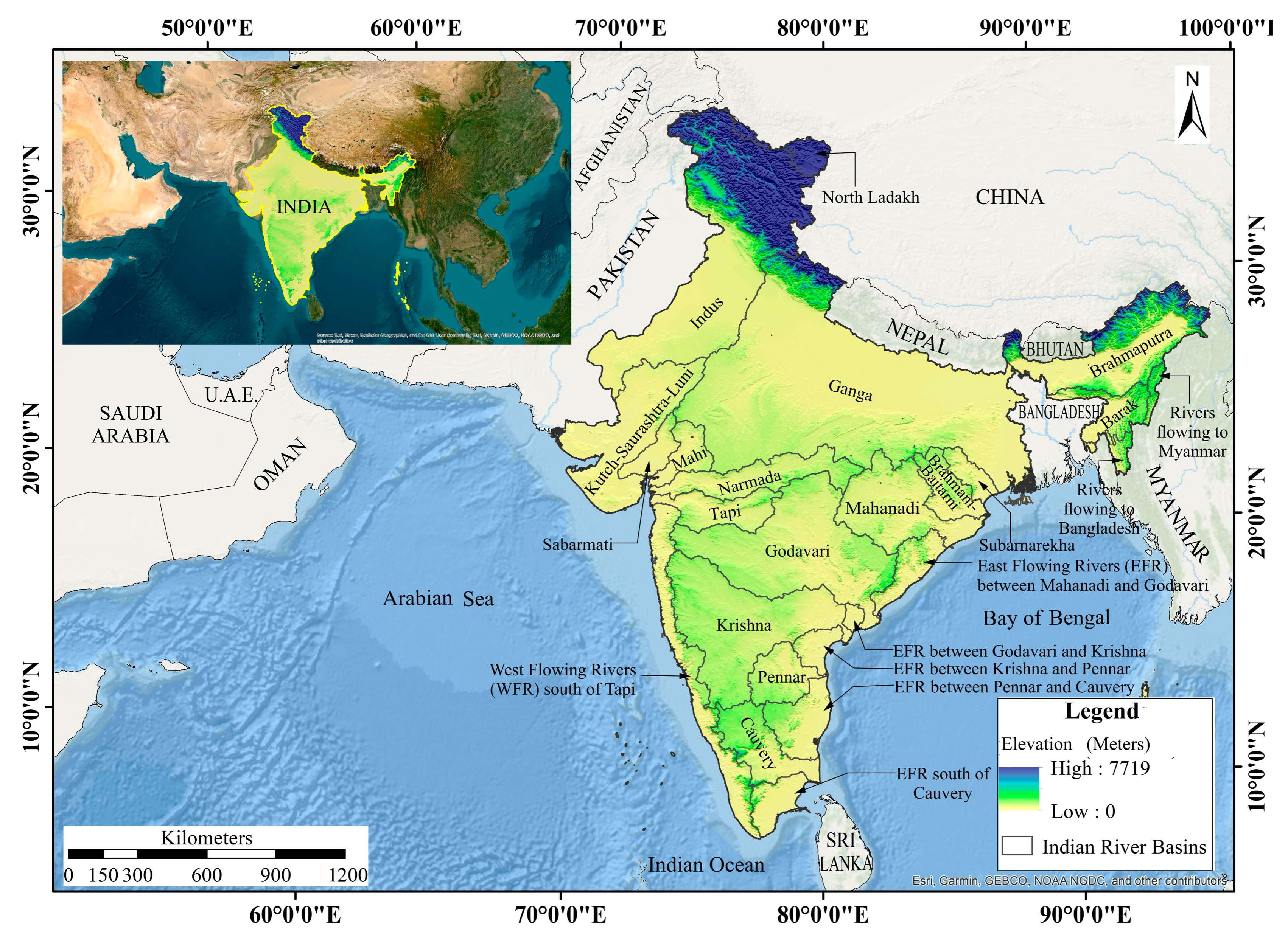
2.1. Study Area

The mainland of India, located within the Asian continent, offers a captivating and diversified landscape that extends from 8°4′ N to 37°6′ N latitude and 68°7′ E to 97°25′ E longitude, entirely north of the equator. India is the 7th largest country globally, accounting for 2.4% of the total land surface area on Earth. India’s vast geographical expanse encompasses a remarkable array of diverse geology, physiography, climate, and ethnicity. In the northern reaches, the dominant presence of the majestic Himalayas gives rise to narrow, energetic streams that carve through the land. It has numerous prominent river systems, including the Ganges, Brahmaputra, Yamuna, Godavari, Krishna, and Cauvery, among others. These rivers have their origins in elevated areas such as the Himalayas, the Western Ghats, and the undulating terrain of the Deccan Plateau. They gracefully traverse the plains before ultimately finding their way into the Bay of Bengal or the Arabian Sea, forming many river basins (Figure 1).
Regions such as the Gangetic Plains and the Western Ghats in India are characterized by the prevalence of sedimentary rocks, including sandstone, limestone, and shale. Meanwhile, the Deccan Plateau is dominated by the extensive basaltic formation known as the Deccan Traps. In Rajasthan, the Aravalli Range showcases ancient Precambrian rocks.
According to the National Bureau of Soil Survey and Land Use Planning, the soils across India display a diverse range of characteristics. The floodplains of major rivers are predominantly composed of alluvial soils, while the Deccan Plateau is known for its black soils, also referred to as vertisols. In regions with high rainfall, red and laterite soils are prevalent. The texture of these soils exhibits varying spatial distribution across different regions of India. Sandy soils dominate in arid and semi-arid areas like Rajasthan, while clayey soils are frequently encountered in the Gangetic plains. Loamy soils, which comprise a blend of sand, silt, and clay, can be found in various parts of the country, including regions of Madhya Pradesh and Maharashtra.
India exhibits an exceptionally varied climate due to its vast geographical extent and diverse topography. The country encompasses six primary climate types, which include tropical monsoon, tropical wet and dry, arid and semiarid, subtropical humid, mountain, and highland [50]. Each of these climate types has distinct characteristics that exert a significant influence on the weather patterns observed across different regions of India. The tropical monsoon climate, in particular, is the most prominent and covers a substantial portion of the country. It is characterized by well-defined wet and dry seasons, with the southwest monsoon, typically occurring between June and September, being responsible for the majority of India’s annual rainfall. Unfortunately, during this season, the combination of heavy silt loads carried by rivers from catchments and the insufficient carrying capacity of the rivers results in backed-up drainage systems, riverbank erosion, and floods in drainage basins. As a consequence, there is a substantial toll on human lives and damage to property, infrastructure, and public services in the most densely populated basins of the most populated country [51]. The escalating flood-related damages are a matter of concern, as floods have occurred in places previously considered not prone to such disasters.

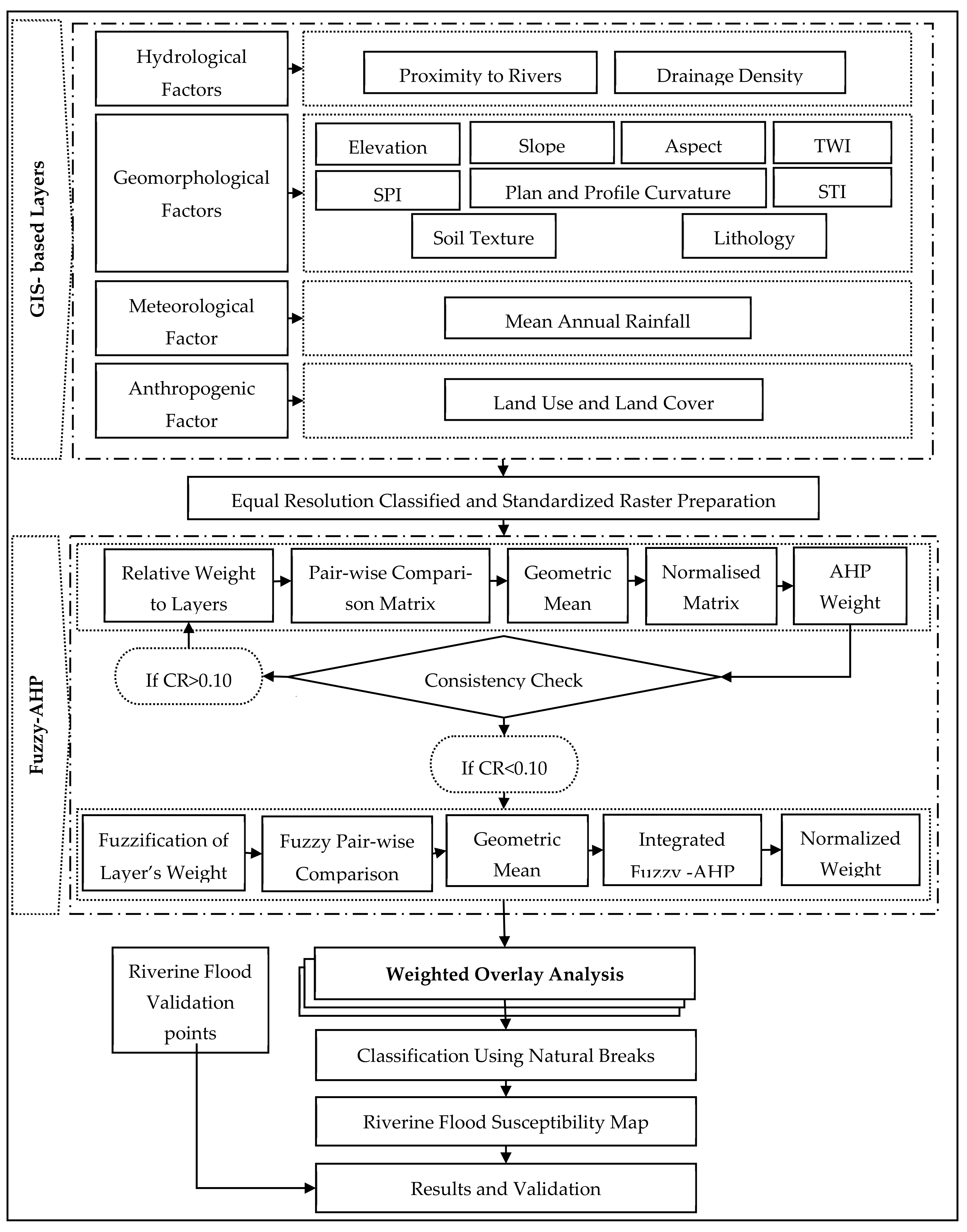
2.2. Database and Methodology

Extensive data on flood conditioning factors and flood validation points were collected at a pan-India level, including geomorphological, hydrological, meteorological, and anthropogenic factors from various sources. Specifications of all the factors, their relation to riverine floods, and factor map preparation methods have been discussed in Table 1. The SRTM DEM was utilized to derive the geomorphological factors, which include elevation, slope, aspect, plan curvature, profile curvature, SPI, STI, and TWI. By employing drainage delineation techniques in ArcGIS 10.8 software using the DEM, layers for the hydrological factors, such as proximity to drainage and drainage density, were generated. Further, vector data pertaining to soil texture, mean annual rainfall, lithology, and land use/land cover (LULC) were extracted from relevant global data sources. These extracted layers were then clipped to the study area to ensure their applicability. To promote consistency and facilitate analysis, all the conditioning layers were resampled into the required format, with a spatial resolution of 2000 m × 2000 m. This resampling process aimed to create a standardized and homogeneous database for further analysis and evaluation. The relative hierarchy of the factors and their classes was then determined to find AHP weights, normalized fuzzy weights, and integrated FAHP weights. A Group of Decision Makers (GDM) panel was formed to select and rank influencing factors. The GDM panel was comprised of five experts, encompassing scientists and professors specializing in disaster studies, hydrology, and climate research. In instances where inconsistencies arose, the responsibility of assigning weights was reallocated to the respective decision-makers to establish coherence. Further, the RFS map was generated by a weighted overlay of the FAHP weights. To assess the accuracy of the RFS map, spatially balanced validation points were created using the United Nations Development Programme’s (UNDP) flood zone map in ArcGIS. These validation points served as reference points for evaluating the precision and reliability of the flood susceptibility assessment. The complete methodology is briefly outlined in Figure 2.

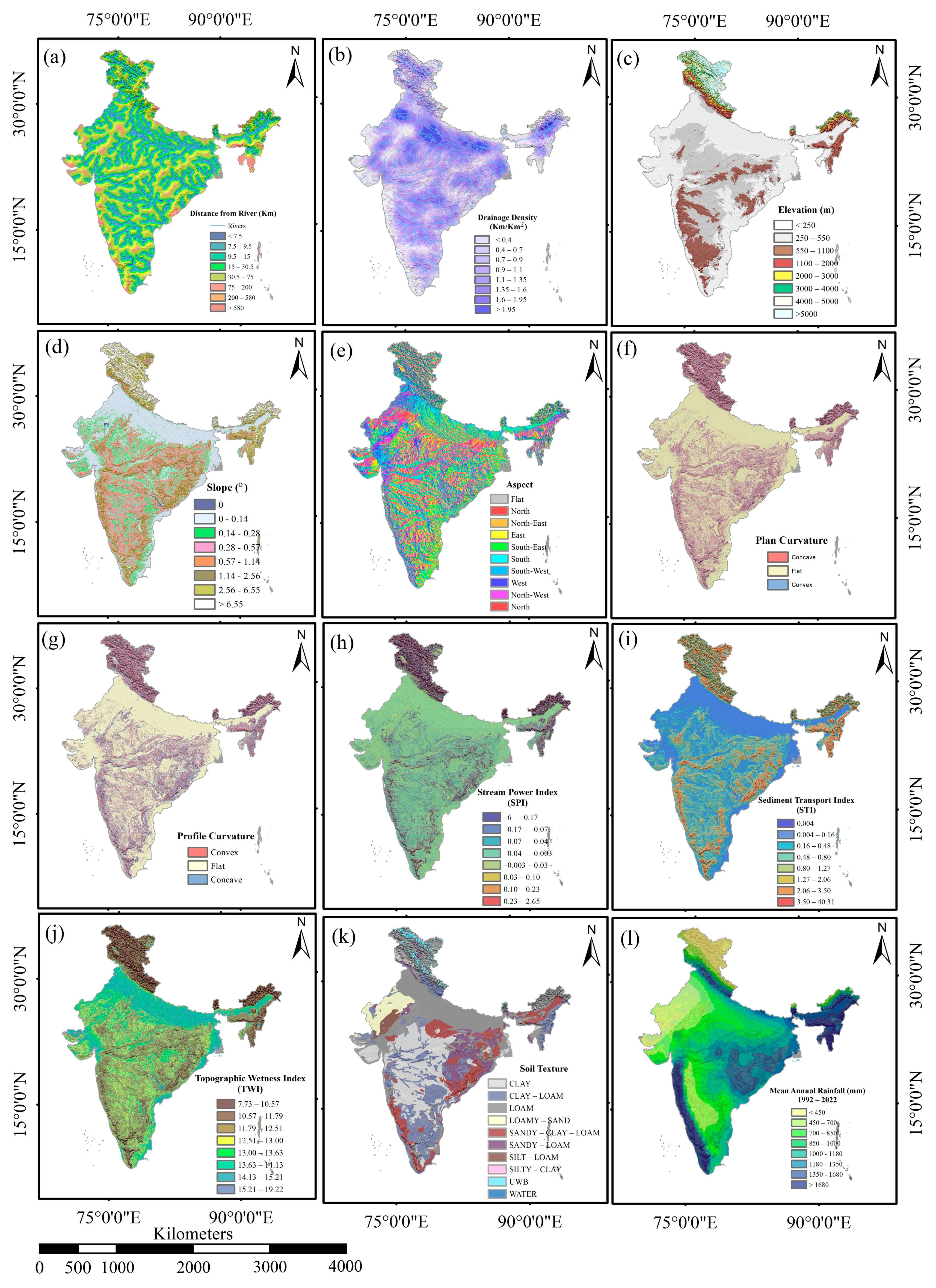
2.2.1. Hydrological Factors

Distance from Rivers is often used as a proxy for flood susceptibility, with areas closer to streams considered to have a higher flood risk [52]. Proximity to drainage is typically measured as the Euclidean distance between a specific location and the nearest stream or river channel [53]. A proximity map can be created using the Euclidean distance or the multiple ring buffer tool. After that, proximity and analysis tools were used to create multiple buffers around river shapefiles in India. The Geometric Interval method under the reclassify tool is then used to divide the proximity to drainage data of India into eight classes because it accounts for the exponential decay of influence as the distance from a drainage feature increases. This method assigns larger intervals to smaller distances, emphasizing the proximity effect, while assigning smaller intervals to larger distances, highlighting the diminishing influence of the drainage feature. Figure 3a depicts the distance from rivers in India.
Drainage density is a measure of the total length of streams and rivers per unit area in a watershed. It indicates the degree of channel development and can provide insights into flood-prone areas [54]. Higher drainage density represents a denser river network, which suggests a higher potential for water accumulation and increased flood risk, and vice-versa [54]. The drainage density map of India has been prepared using the Line Density tool in ArcGIS. The quantile method was used to divide the drainage density data of India into eight classes because it makes equal-sized groups by distributing an equal number of observations in every class [55]. Figure 3b represents the drainage density map of the country.

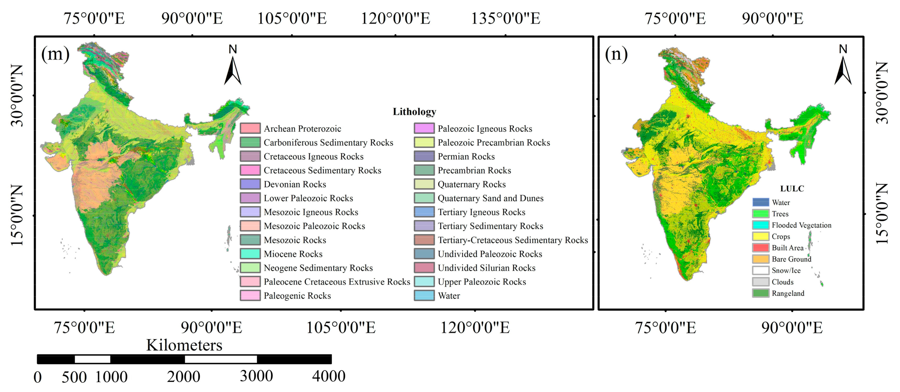
2.2.2. Geomorphological Factors

Elevation plays a crucial role in RFS as it determines the height and position of the land in relation to the water level. Low-lying areas with lower elevations are more prone to flooding compared to higher elevations [56]. SRTM DEM was used to extract the elevation map of India, which was further classified in ArcGIS using the reclassify tool (Figure 3c). The natural breaks method was employed for this classification because it is highly efficient in identifying significant and distinguishable classes within the data by minimizing variation within groups and maximizing variation between groups [57].
Slope is the degree of inclination or steepness of the land’s surface, which is defined by the ratio of vertical change (rise) to horizontal distance (run) [58]. Steeper slopes tend to generate greater velocity, allowing runoff to be quickly carried away. In contrast, runoff on gentle slopes or flat terrain tends to be retained and released gradually over time [59]. The slope map for India was generated using the slope in ArcGIS (Figure 3d). The planar method was applied, using the SRTM DEM dataset as the input. After generating the slope map of India, it was further divided into eight classes using the quantile method.
Aspect refers to the orientation of a slope or the inclination of a land surface in relation to the cardinal directions, such as north, northeast, and the remaining six directions [60]. It plays a significant role in determining the exposure of the land to solar radiation, which in turn affects soil moisture and vegetation patterns, which influence the susceptibility of an area to flooding [61]. To generate the aspect map of India, the planar method in the aspect tool was used in ArcGIS (Figure 3e). Furthermore, it was reclassified into eight classes using defined the interval method.
Plan Curvature is the rate of change in slope along a contour line, which denotes the horizontal curvature of the slope of the land surface [62]. It can affect the flow of water across the landscape, influencing the direction and accumulation of runoff, which can contribute to increased flood risk [59]. Areas with concave shapes tend to accumulate water, increasing the likelihood of flood occurrence [63]. SRTM DEM was used in ArcGIS to build the plan curvature map for India (Figure 3f). The plan curvature of India was reclassified into three classes using a defined interval.
Profile Curvature is the vertical curvature of a land surface, indicating the degree of change in slope along the direction of the steepest slope [62]. It is a key factor in determining RFS zones as it influences the flow dynamics and the likelihood of channel overbanking. Positive profile curvature indicates concave slopes, which can lead to flow convergence and increased flood risk, while negative profile curvature represents convex slopes that facilitate flow divergence and reduce flood susceptibility [64]. Using the curvature tool, the SRTM DEM was processed on ArcGIS to produce the profile curvature map of India (Figure 3g). The profile curvature of India was separated into three classes using a defined interval.
Stream Power Index (SPI) is a quantitative measure that determines the erosive power of flowing water in a river or stream. It combines the slope and drainage area to estimate the potential for sediment erosion and transport [65].
Stream Power Index, SPI = As × tanβ
where specific catchment area is represented by As and the slope angle is represented by β.
High SPI values indicate areas with higher energy and potential for erosion, which can contribute to increased flood susceptibility [66]. Equation (1) was used on a raster calculator available within the spatial analysis tool to create the SPI map of India (Figure 3h). The quantile method under the reclassify tool was used to divide the SPI data of India into eight classes because it creates equal-sized groups by distributing an equal number of observations in every class.
Sediment Transport Index (STI) is a measure of a river’s ability to transport sediment. It considers factors such as stream power, slope, and sediment supply to estimate the potential for erosion and sediment movement [67]. Sediment transport influences channel capacity, morphology, and sedimentation patterns, which can influence floodplain storage and flood dynamics [68]. Figure 3i depicts the study region’s STI map.
Topographic Wetness Index (TWI) is a measure of landscape wetness derived from topographic parameters, such as slope and contributing area. It estimates the potential for water saturation and indicates areas prone to water accumulation and soil moisture [69].
TWI = Ln (X/tanβ)
where the specific contributing area is represented by X and the slope gradient is represented by β [69].
Areas with higher TWI values indicate higher water accumulation potential, which can contribute to increased flood susceptibility [70]. Equation (2) was used on a raster calculator to create the TWI map of India (Figure 3j). The quantile method under the reclassify tool was then used to divide the SPI data of India into eight classes because it creates equal-sized groups by distributing an equal number of observations in every class.
Soil texture refers to the proportionate representation of sand, silt, and clay particles in the soil, which affects water infiltration rates and soil moisture holding capacity and could influence flood runoff characteristics [71]. Fine-textured soils (e.g., clay) have a lower infiltration capacity, leading to increased surface runoff and potential flooding, while coarse-textured soils (e.g., sand) tend to drain more quickly [56]. The soil texture map of India was extracted from the FAO World Soil Data (Figure 3k).
Lithology is the physical characteristics and composition of rocks or sediments in a particular area. Different permeabilities of rocks affect the infiltration and groundwater storage capacity, which can affect surface runoff and flood susceptibility [72]. The lithology of India was clipped from the world lithology data provided by USGS (Figure 3m).

2.2.3. Meteorological Factor

Mean Annual Rainfall is an essential parameter for understanding flood frequency and hydrological processes [73]. Higher mean annual rainfall can contribute to increased flood susceptibility due to greater water input and runoff potential [74]. The precipitation data for the past 30 years (1991–2021) was obtained from CRU in NetCDF file format. It was initially transformed into a raster format and subsequently converted into a point format using the conversion tool within ArcGIS. The data underwent further processing, including the conversion of the point data into mean annual rainfall data using the cell statistics tool. Afterward, the point data for the entire world was subjected to interpolation. Subsequently, the dataset was narrowed down to India through a clipping process. The mean annual rainfall data specific to India were then categorized into eight classes using the quantile method. Figure 3l visually represents the resulting map of mean annual rainfall.

2.2.4. Anthropogenic Factor

LULC delineates the physical and functional features of the Earth’s terrain, including vegetation, urban areas, water bodies, and other land types. LULC patterns influence surface runoff, infiltration, and flood dynamics [75]. Urban areas, for example, on impervious surfaces tend to have higher flood susceptibility compared to naturally vegetated areas [76]. The LULC map of India was clipped from the world LULC data provided by Sentinel 2A (Figure 3n).

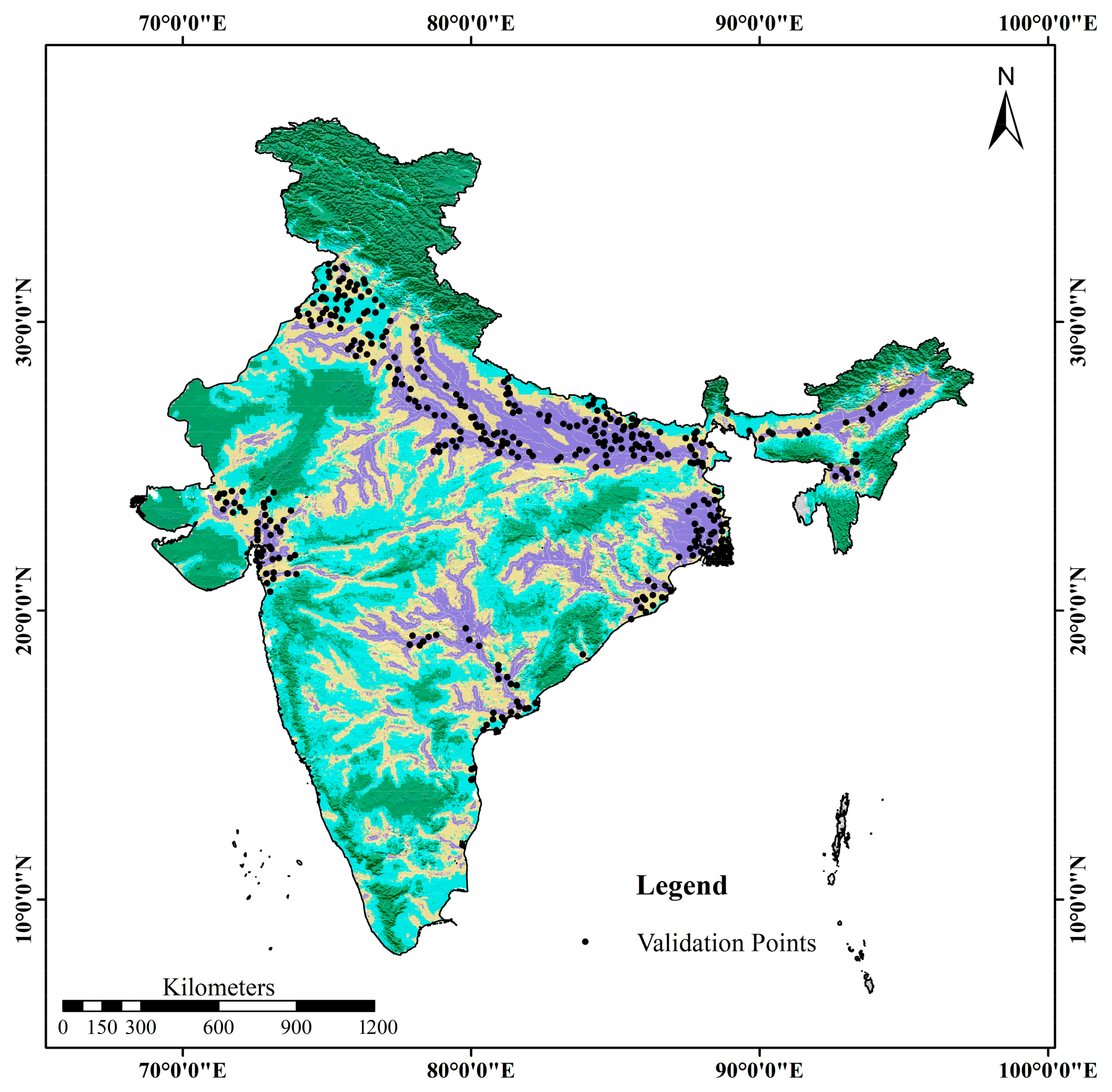
2.3. Validation Points

A flood inventory map is a geographical depiction that documents and captures the scope, attributes, and consequences of past flood incidents within a defined region [77]. As stated by [78], flood inventory data are vital for training datasets and assessing the precision of flood susceptibility models. The flood inventory map was created using the create spatially balanced points tool in ArcGIS, utilizing the UNDP flood zone map. Through this tool, a total of 364 flood locations were identified.

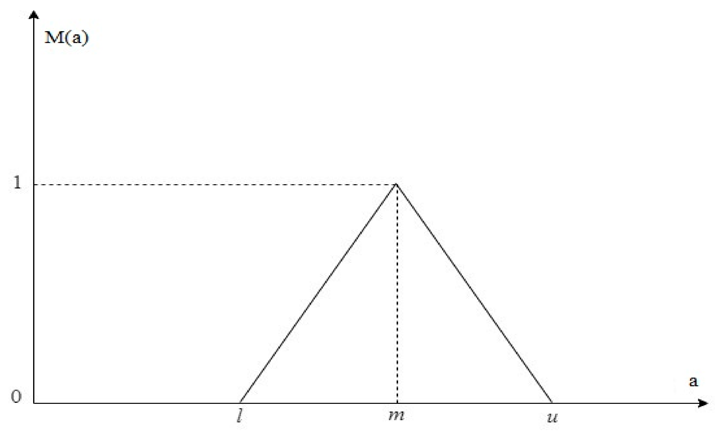
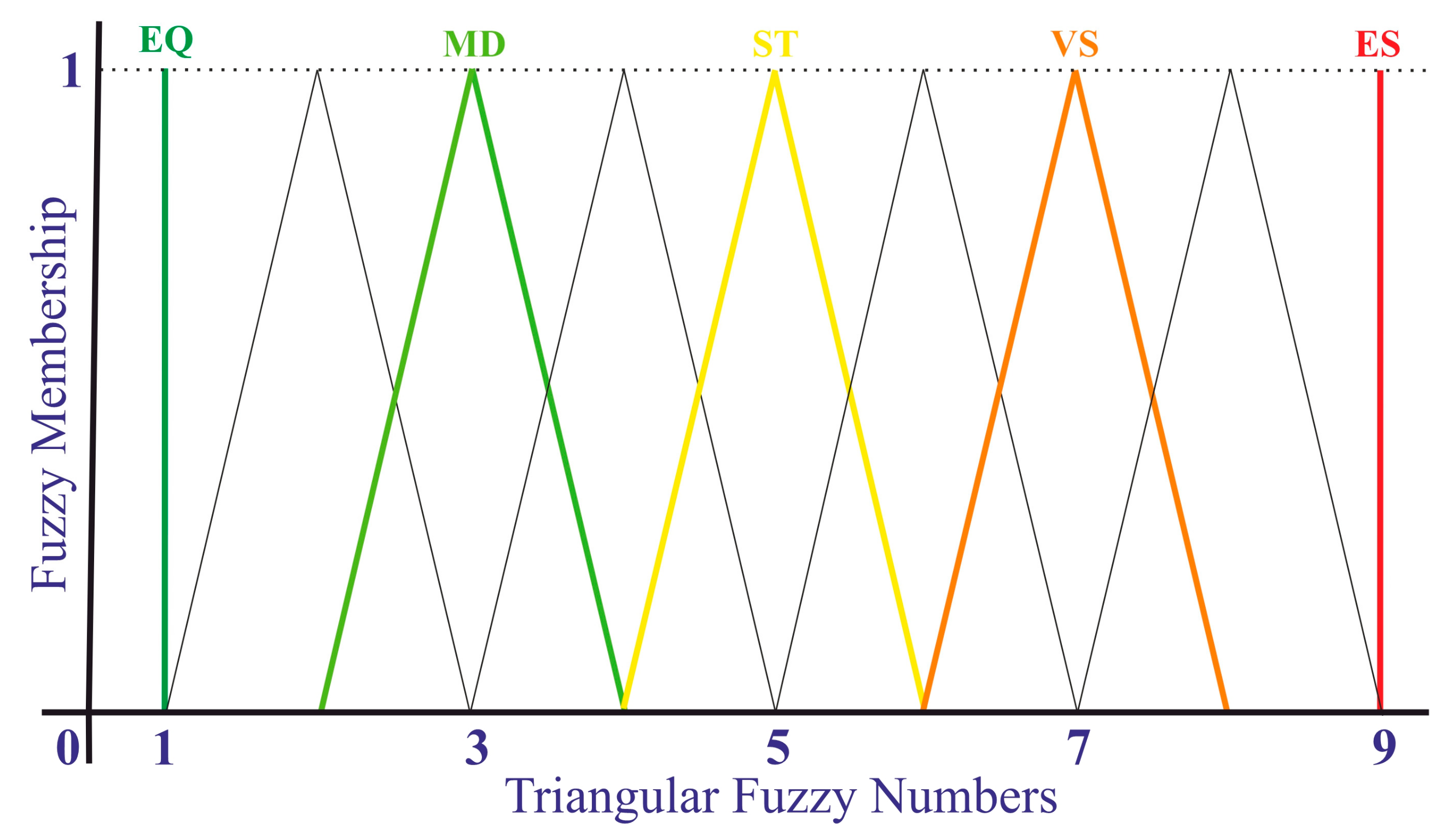
2.4. Fuzzy Analytical Hierarchy Process (FAHP)

The AHP, originally developed by [45], offers a structured approach to address multicriteria decision problems [79]. It relies on paired comparisons that use hierarchical structures to depict a problem and subsequently establish relative priorities for a huge number of criteria and alternatives through the subjective judgments of a user [45]. AHP is recognized as a potent tool in the field of hazard management [80]. Ref. [81] stated that a fundamental benefit of AHP is its capacity to reconcile discrepancies (inconsistencies) in a marginal percentage, its reliance on judgment data, and the availability of several commercial software that aid in simpler computations.
Fuzzy numbers set X ~ in A ⊆ R, where R represents real numbers’ set, and can be explained in the form of ordered pairs X ~ i n = {a, µ X ~ (a)}, where ‘a’ belongs to A and µ X ~ (a): A → [0, 1]. The function µ X ~ (a) denotes the membership function (MF) of X ~ , which assigns a degree of membership ranging from 0 to 1 to each object ‘a’ [82,83]. A special type of normalized fuzzy set is referred to as a fuzzy number. Fuzzy numbers come in various forms, with triangular and trapezoidal shapes being the most common and useful. Trapezoidal fuzzy numbers are particularly useful when dealing with more complex situations involving ambiguity in decision-making analysis, while TFN are favoured in MCDM techniques due to their simplicity, ease of interpretation, and applicability in handling uncertainty. They effectively capture imprecision in decision-making processes by representing a range of possible values using a triangular distribution. This enhances decision models’ ability to handle real-world uncertainty [84]. In this study, Buckley’s TFN was employed to assign the fuzzy weights to the factors using analytical conversion operations (Table 2). The TFN is graphically depicted in Figure 4, which is also the membership function given by [85] used for the representation of fuzzy linguistic concepts in this study.
The FAHP is an integrated approach that combines qualitative and quantitative methods. Interestingly, the concepts of fuzzy sets have found application in various MCDM techniques, including fuzzy TOPSIS (Technique for Order of Preference by Similarity to Ideal Solution) as demonstrated by [86], and fuzzy PROMETHEE (Preference Ranking Organisation Method for Enrichment of Evaluations) as discussed by [87]. In the context of FAHP, the linguistic terms employed for comparing pairs of factors can be translated into numerical values using Saaty’s 1–9 scale. Table 2 depicts the comparative values of the influence of factors on Saaty’s and TFN scales. This process is complemented by a corresponding conversion scale for fuzzy numbers indicating relative importance, as outlined by [85,88].
The FAHP approach is used in this work to investigate RFS. The FAHP approach was designed and structured in the following steps:
Step-1: Establishing the purpose, hierarchy, and identity of each susceptibility component and its subcomponent;
Step-2: Preparation of the pair-wise comparison matrix based on Saaty’s scale (Table 2), [xk], the elements of which [ x ~ ij]k depict the preference of the kth expert for the risk factor i over the risk factor j; i, j ∈ N. The basic relationship between the elements of the reciprocal matrix is ( x ~ ij) · ( x ~ ji) = 1 [89].
Step-3: Using Equation (3), create the mean pair-wise comparison matrix, [x], with components representing the average values of experts’ opinion:
X i j = x i j 1 + x i j 2 + + x i j k k k : number of experts involved
Step-4: AHP weight was calculated and validated on the basis of the Consistency Ratio (CR). In this case, CR is greater than 0.10; the matrix was revised, and further weights were calculated to make sure that CR is less than 0.10. CR is calculated using Equation (4).
CR = CI RI ( n )
where CI = ( λ max n ) n 1 ; λ = eigenvalue of the pairwise comparison matrix; n = number of vulnerability factors; RI = Random Index (Table 3).
Step-5: Construction of the fuzzy pairwise comparison matrix [ X ~ ] with fuzzy values, X ~ ij utilizing the linguistic scale of the membership function and TFN numerical conversion procedures (Table 2, Figure 5).
Step-6: Estimation of the fuzzy geometric mean value for each risk factor Gi, as per Buckley’s methodology (Equation (5)):
G i = j = 1 n X ~ i j 1 n = ( X ~ i 1 X ~ i 2 X ~ i 3 X ~ i n ) 1 / n
After the calculation of the fuzzy geometric means, the fuzzy geometric susceptibility vector factors are estimated (Equation (6)):
G = [ G 1 , G 2 , G 3 , , G n ] T
Step-7: Definition of the fuzzy susceptibility factors (i.e., the fuzzy relative weights, FRW) WRi, according to Equation (7):
W R i = G i ~ j = 1 n G j 1 = G i ~   G ~ 1   G ~ 2   G ~ 3     G ~ n 1
Step-8: Defuzzification of the FRW, WRi, for evaluating the crisp values Wi, by adopting the centroid of the area (CoA) approach using Equation (8):
W i = l · W i + m · W i + u · W i 3
Step-9: Normalisation of the de-fuzzified relative weights Wi using Equation (9):
W N i = W i / ( i = 1 n W i ) W i = 1 W i > 0

2.5. Flood Susceptibility Mapping

Upon establishing the relative weight of each criterion and its sub criterion, it was multiplied by 100 prior to the calculation of the flood susceptibility index (FSI) within the GIS. The FSI values were estimated using ArcGIS. Equation (10) was used to complete this procedure:
F S I = i = 1 n W i F × G i F
where W i F is the weight of each component, G i F denotes the rank value of subcategories, and n represents the number of factors.

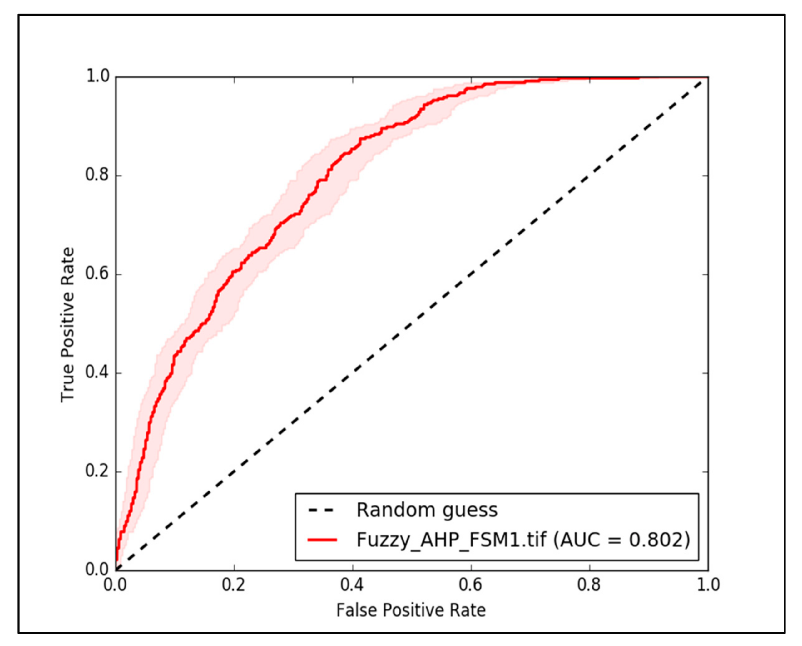
2.6. Validation Using AUROC Analysis

Assessing the accuracy of output models derived from any MCDM approach is a crucial aspect. The evaluation of these models can be effectively accomplished using the AUROC analysis, which relies on incidence data (specifically historical floods in this study) [90]. The AUROC analysis is widely recognized for its simplicity, comprehensiveness, and reasonable alignment with predictions [91]. The AUROC is generated by finding the ratio of sensitivity (true positive rate) and specificity (false positive rate) using the ArcSDM toolset in ArcGIS. The value of the curve ranges from 0.5 to 1, which is classified into five categories: poor (0.5–0.6), moderate (0.6–0.7), good (0.7–0.8), very good (0.8–0.9), and excellent (0.9–1) performance [92]. Based on the data, the area below the curve was calculated numerically using the following Equations (11) and (12):
Sensitivity = TP TP + FN
Specificity = TN FP + TN
where, TP: True Positive; TN: True Negative; FP: False Positive; and FN: False Negative
ROC = Sensitivity Specificity

3. Results

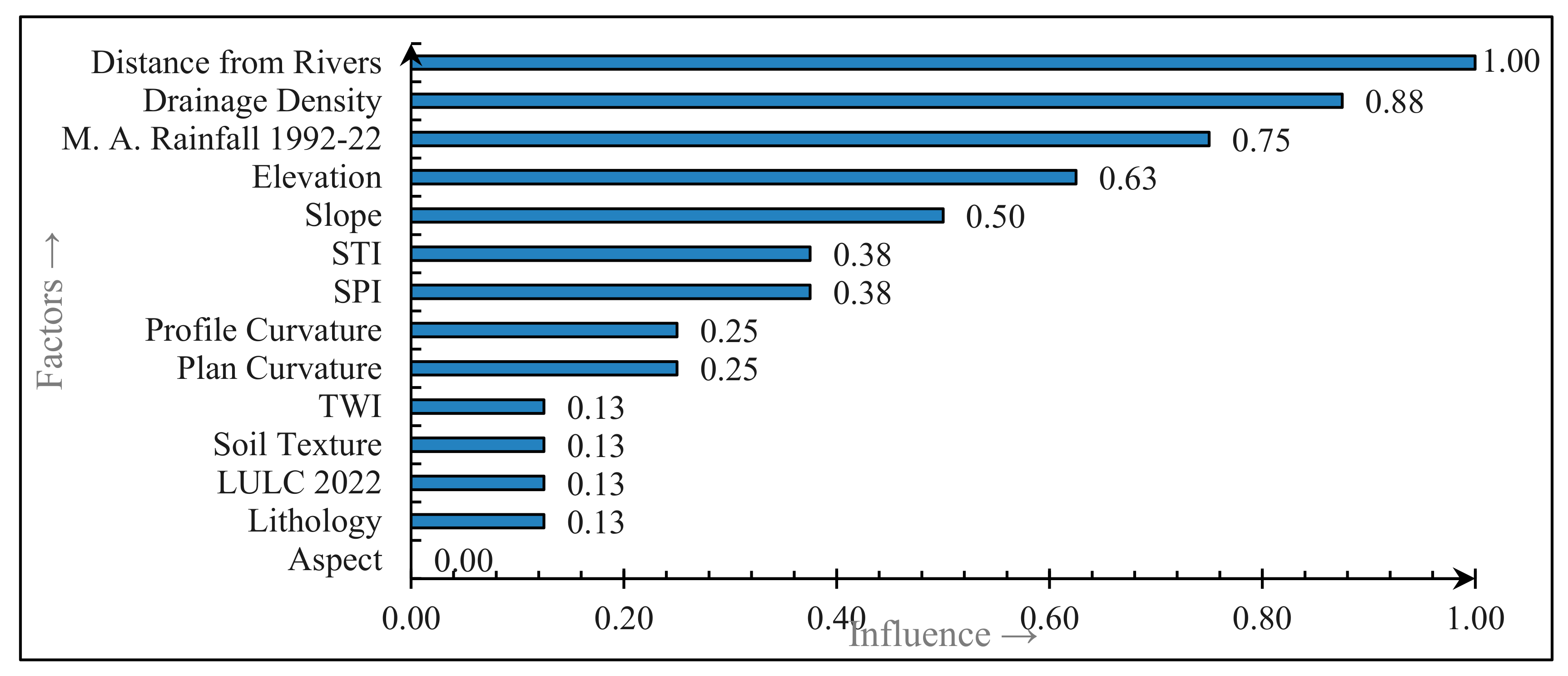
3.1. Influence of Factors on Riverine Floods

The significance of each factor in relation to riverine floods was determined through the computation of mean weights for factors affecting riverine floods, drawing from GDM weights as presented in Table 4.
It is found that the distance from rivers emerged as the most influential criterion, exerting a 100% impact, followed by drainage density at 87.5%, mean annual rainfall at 75%, elevation at 62.5%, slope at 50%, SPI and STI at 37.5%, and plan and profile curvature at 25%. Further down the list was lithology, LULC, soil texture, and topographic wetness index (TWI) at 12.5% and the factor with the least influence was aspect (Table 4, Figure 6).
In cases of major flood conditioning factors, it is found that the parts of the study area within 7.5 km of rivers, having a drainage density greater than 1.5 km/km2, and having mean annual rainfall of more than 167 cm are highly susceptible to riverine flooding. This scenario is further influenced by elevation being less than 260 m, slope less than 0.14°, SPI greater than 0.10, STI in the range of 3.50–0.31 and TWI in the range of 15.18–19.22. Areas with clayey soil texture, Mesozoic igneous rock lithology, and LULC types associated with water bodies and their adjacent areas are identified as being more susceptible to flooding in this scenario. Aspect holds the least sway in influencing riverine floods, with the west-facing flanks exhibiting more susceptibility. Ranks for the classes of each conditioning factor are given in Table S1.

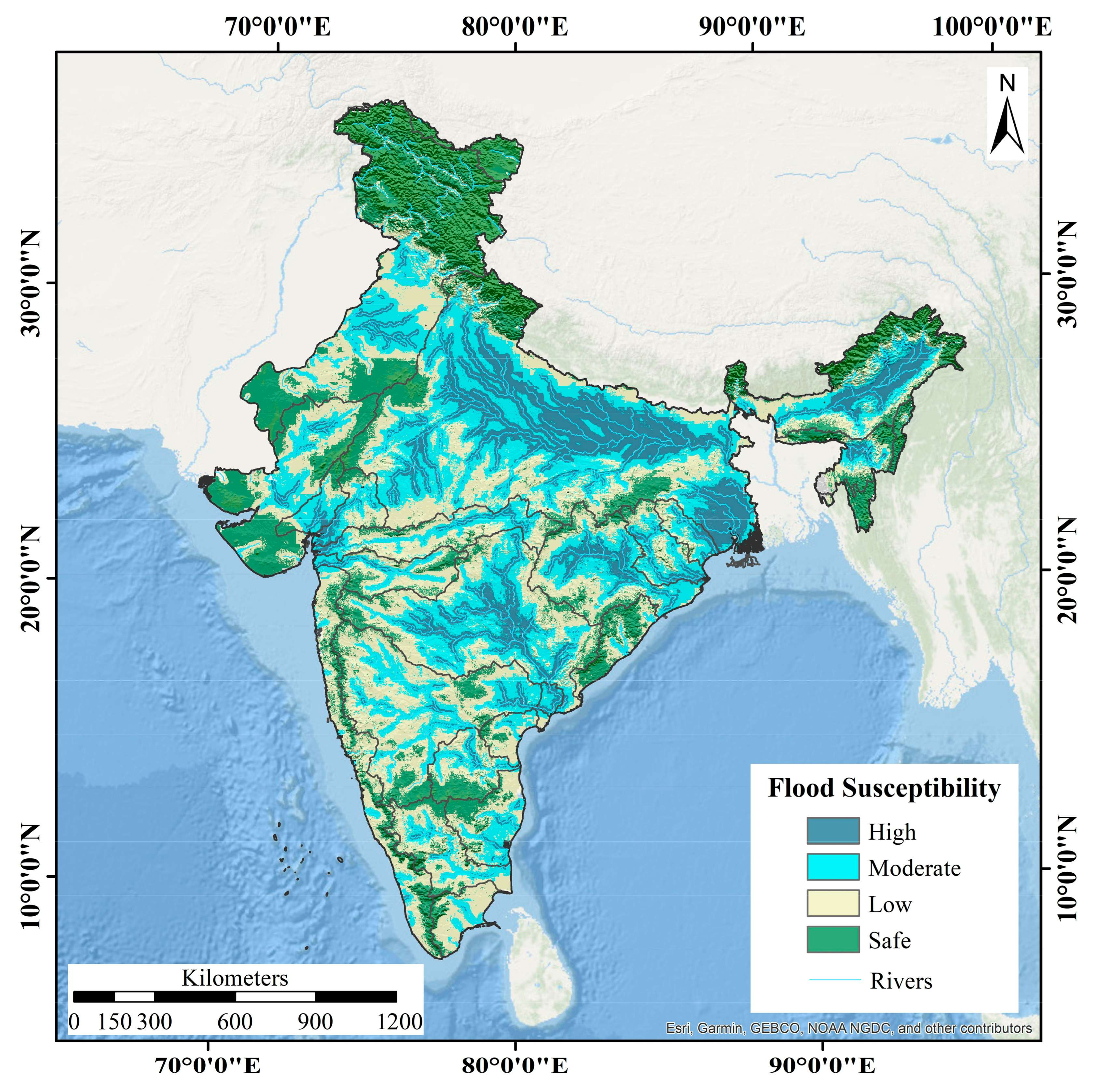
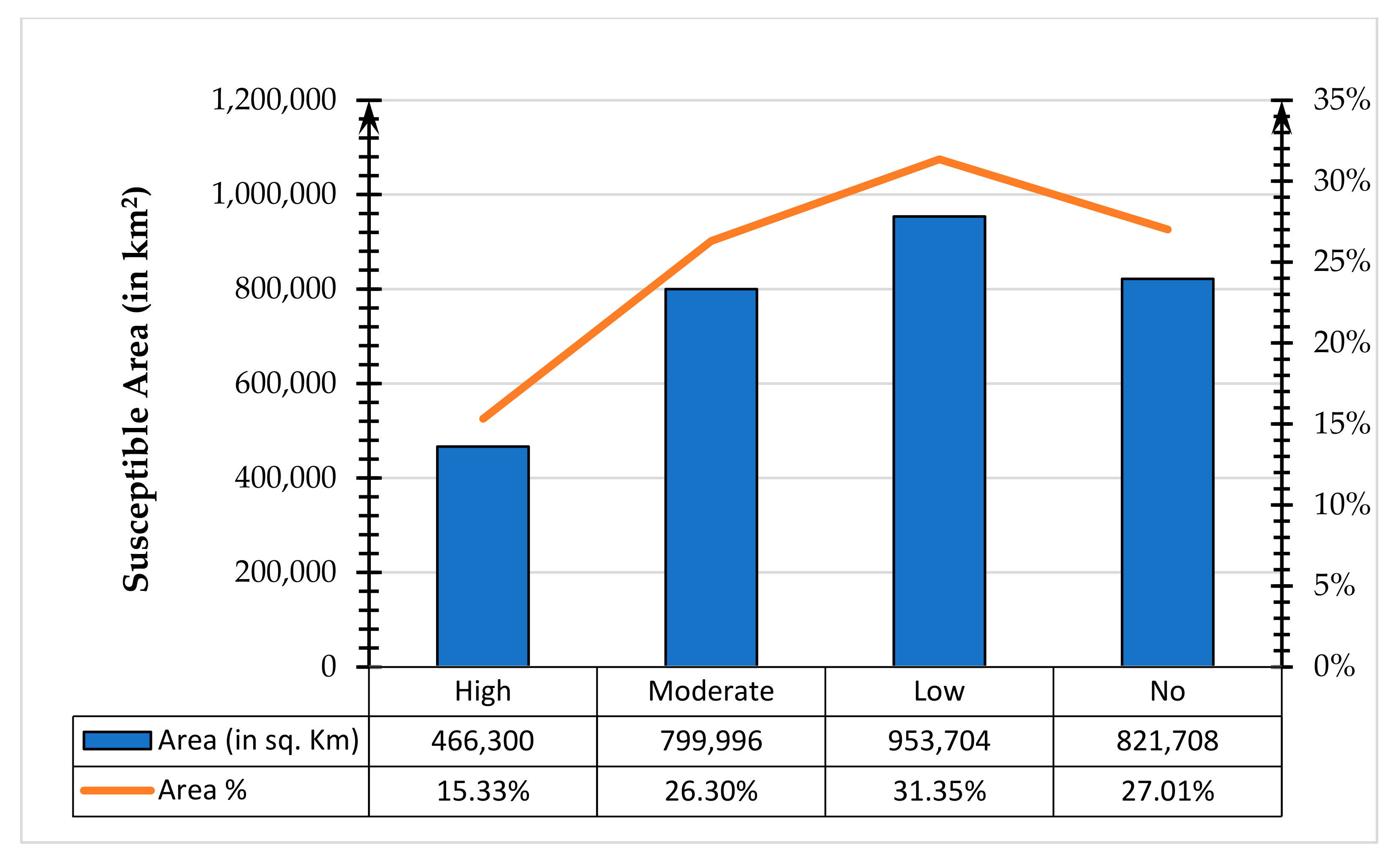
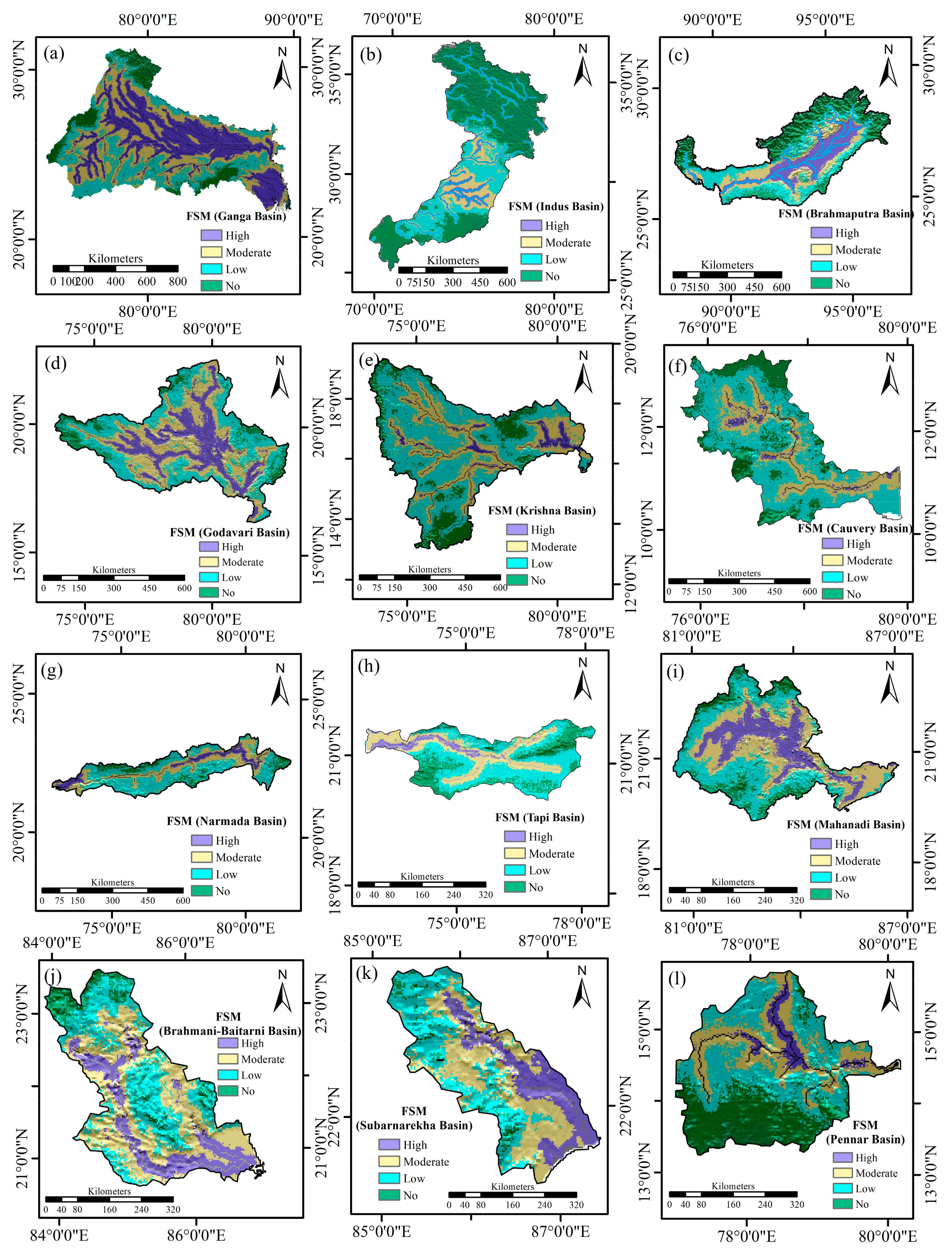
3.2. Flood Susceptibility Zonation

In this study, to synthesize the RFS zonation map of India using the FAHP, the AHP pair-wise comparison matrix (Table S2) was fuzzified using TFN analytical conversion operations, detailed in Table 2. Subsequently, FAHP geometric means, fuzzy weights, and normalized weights for the conditioning factors were derived using Equations (5)–(9), as presented in Table 5. The normalized weights were integrated with the raster layers and combined in accordance with Equation (10) to produce the RFS map of India. To enhance the map’s clarity, the RFS was classified into four distinct categories using the natural break method. This classification approach was chosen due to the region’s varied topography and expansive geographical coverage, resulting in the production of the RFS map, vividly illustrated in Figure 7.
The RFS map classification yielded four zones of flood susceptibility, i.e., high, moderate, low, and no flood susceptibility. Notably, the distribution of these zones across the country is such that 466,300 km2 (15.33%) area falls in the high flood zone, 799,996 km2 (26.30%) area in the moderate flood zone, 953,704 km2 (31.35%) area in the low flood zone, and 821,708 km2 (27.01%) area in the no flood susceptibility zone (Figure 8). To ascertain the accuracy of these zones, rigorous validation was performed through the area under the receiver operating characteristic curve (AUROC) analysis, leveraging true positive points as benchmarks.

3.3. Flood Susceptibility Validation Using AUROC Analysis

The validation process for the RFS map generated using the GIS-based FAHP technique encompassed the application of AUROC analysis. The validation data points were extracted from the UNDP flood zone map of India (Figure 9). The RFS Map, generated as a result of this investigation, demonstrates a noteworthy level of predictive accuracy at 80.2% (Figure 10). Based on the considerable level of precision attained, it is reasonable to deduce that the outcomes of the RFS Map, which was produced using the GIS-based FAHP methodology, possess a strong degree of reliability and are capable of providing credible forecasts. This highlights the efficacy of our technique in assigning weights to different contributing elements and doing subsequent computations, which have successfully delineated the actual levels of susceptibility throughout the research region.
The AUROC validation has yielded an accurate score in terms of relating the product of this study to the UNDP flood zone map of India, thereby reinforcing the credibility of our research findings. Notably, this study took a more holistic approach, incorporating a broader spectrum of factors, including geomorphological, hydrological, meteorological, and anthropogenic aspects, to determine flood-susceptible zones, unlike the UNDP flood zone map and the National Remote Sensing Centre’s (NRSC) flood susceptibility assessments, which are primarily focused on historical flood events. This comprehensive analysis provides invaluable insights into flood-prone regions across various parts of India, offering a detailed understanding of the intricate dynamics that govern riverine floods in India.

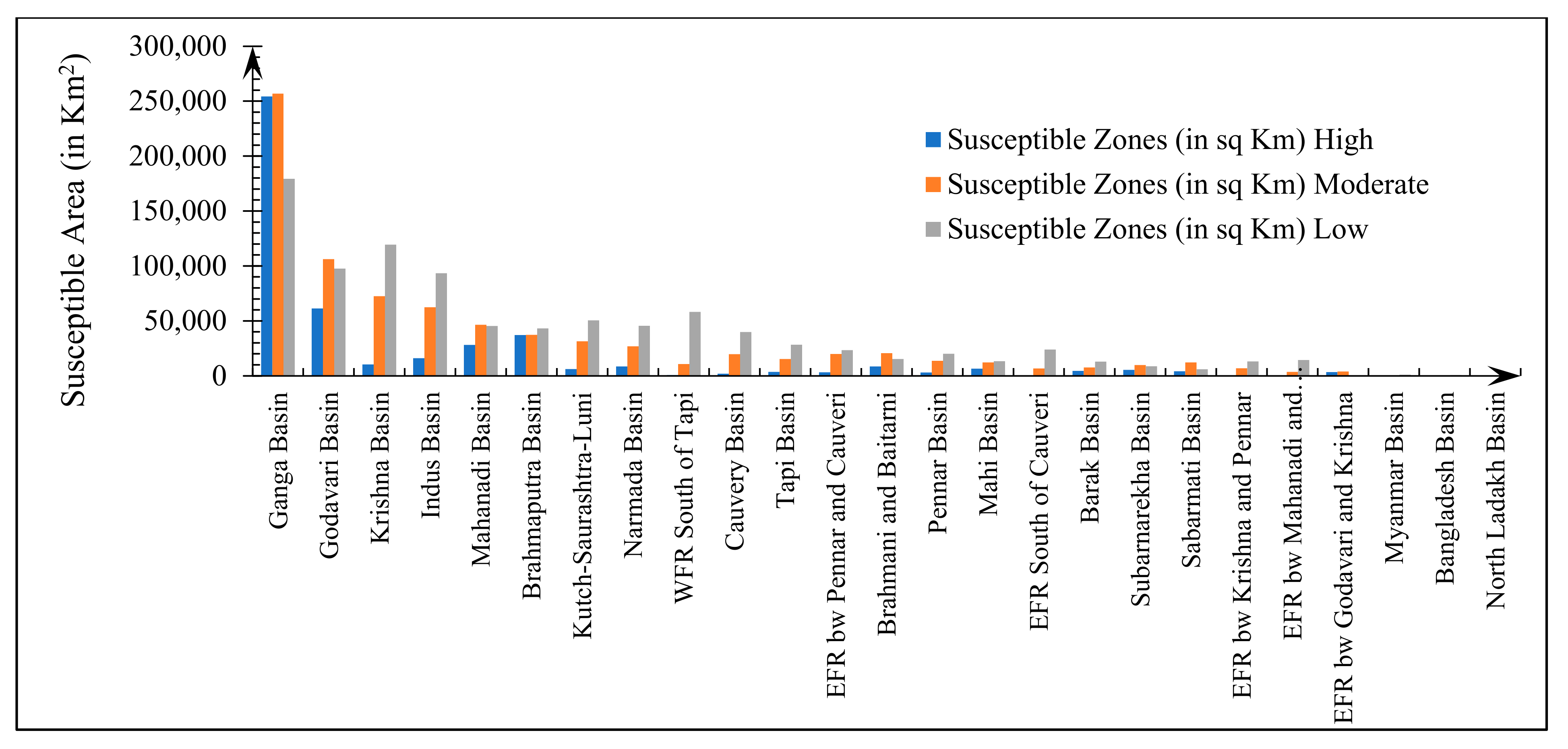
3.4. Riverine Flood Susceptibility (RFS) Assessment of Indian River Basins

The vast country of India is divided into 24 river basins, of which Ganga, Brahmaputra, Indus, Godavari, Krishna, Mahanadi, Cauvery, Narmada, and Tapi are delineated as the major river basins of the study area. The area of zones of susceptibility of all the basins separately was found using the ‘Tabulate Area’ tool. The susceptibility of Indian river basins to riverine floods is summarized in Table 6, complemented by visual representations in Figure 11, Figure 12 and Figure S1.
The Ganga Basin is the largest basin in India, covering 777,308 km2, and is ranked among the world’s most densely populated basins; it faces significant susceptibility to riverine floods. In this basin, the distribution of RFS zones is as follows: 254,296 km2 (32.71%) high, 256,740 km2 (33.03%) moderate, 179,304 km2 (23.07%) low, and 86,968 km2 (11.19%) no susceptible zone (Table 6, Figure 11a). This basin features the highest proportion of its expanse across the high susceptibility zone, resulting in substantial annual losses in terms of human lives, property, and agricultural output. Highly dense settlements in proximity to many rivers, high drainage density, substantially high rainfall, and the majority of the basin in a very low elevation zone have rendered a considerable portion of the basin at high risk.
Indus Basin spanning an area of 432,276 km2, has 16,132 km2 (3.73%), 62,488 km2 (14.46%), 93,304 km2 (21.58%), and 263,280 km2 (60.91%) of this basin fall into high, moderate, low, and no susceptible zones, respectively (Table 6, Figure 11b). This basin boasts the most extensive region protected from riverine flooding due to its location in an area characterized by scanty rainfall. A substantial 86% of its expanse is situated in low susceptibility and no susceptible zones, rendering it safe against riverine flooding.
Brahmaputra Basin stands as one of the most significant basins on a global scale, yet merely 175,380 km2 of its area lies within India’s borders (Table 6). This central part of the basin has a low elevation, which exhibits a moderate to high drainage density. Its susceptibility to riverine floods is amplified due to the interplay of high sedimentation and substantial precipitation. Within the basin, approximately 67% of the area is prone to flooding, in which 37,184 km2 (21.20%), 37,344 km2 (21.29%), and 43,112 km2 (24.73%) are in the high, moderate, and low susceptibility zones, respectively, while 57,740 km2 (32.92%) area of the basin falls in no susceptible zone (Table 6, Figure 11c).
Godavari Basin is the largest basin (292,044 km2) of peninsular India and the third largest basin of India (Table 6). The distribution of RFS zones in this basin is as followed: 61,368 km2 (21.01%) high, 106,192 km2 (36.36%) moderate, 97,676 km2 (33.45%) low, and 26,808 km2 (9.18%) no susceptible zone (Table 6, Figure 11d). Low proximity to rivers, moderate to high drainage density, high mean annual rainfall, and the presence of clayey and clay-loam soil in the central and southeastern part of the basin make the aforesaid parts of the basin highly susceptible to riverine floods.
Krishna Basin, the second largest basin in peninsular India, spans an extensive 243,968 km2 (Table 6). Of this area, 10,316 km2 (4.23%), 72,428 km2 (29.69%), 119,496 km2 (49.98%), and 41,728 km2 (17.1%) are distributed across high, low, moderate, and no susceptible zones, respectively. Despite its considerable proximity to rivers and a relatively high drainage density, the basin’s unique characteristics result in half of its total area falling into the category of low susceptibility. This can be attributed to the region’s limited rainfall (440–850 mm) and higher elevation range (250–1000 m). Only a small section in the eastern part of the Krishna Basin is classified as a high susceptibility zone (Figure 11e).
Mahanadi Basin covers an area of 138,824 km2, which is positioned to the south of the eastern Ganga basin (Table 6). The spatial distribution of RFS zones within this basin is outlined as follows: 28,124 km2 (20.26%) are designated as high susceptibility, 46,484 km2 (33.48%) as moderate susceptibility, 45,348 km2 (32.67%) as low susceptibility, and 18,868 km2 (13.59%) as non-susceptible zones (Table 6, Figure 11i). Despite having moderately low proximity to rivers and drainage density, more than half of the area of the basin, specifically its central and eastern segments, exhibits significant susceptibility to riverine floods. This susceptibility can be attributed to the combination of high mean annual rainfall (1000–2000 mm) and low elevation (<500 m) prevalent in the central and eastern parts of the basin.
Narmada Basin is centrally located in the western region of India, encompassing an area of 91,924 km2 (Table 6). Within this basin, the distribution of RFS zones is as follows: 8536 km2 (9.29%) high, 26,912 km2 (29.28%) moderate, 45,596 km2 (49.6%) low, and 10,880 km2 (11.83%) no susceptible zone (Table 6, Figure 11g). Predominantly, vast areas of the basin occupy low susceptibility zones due to factors such as a low drainage density (<0.7 km/km2), moderate distance from rivers, and relatively elevated terrain ranging from 260 m to 1200 m. The Narmada River, except for its central portion, has varying susceptibility to riverine floods. The eastern and western areas within 15 km from the banks are highly susceptible, while the central part has a moderate susceptibility due to lower rainfall.
Cauvery Basin is situated to the south of the Krishna basin in the leeward side of the Western Ghats, covering an impressive 78,228 km2. Within this basin, the RFS zones are distributed as follows: 1980 km2 (2.53%) were categorized as high susceptibility, 19,676 km2 (25.15%) as moderate susceptibility, 39,796 km2 (50.87%) as low susceptibility, and 16,776 km2 (21.45%) as non-susceptible zones (Table 6). A significant portion of the basin, accounting for more than half its total area, falls within the low susceptibility zone because of factors, including a moderate to very high distance from rivers, moderately low drainage density, a notably low mean annual rainfall range (436–856 mm), and relatively elevated terrain spanning from 550 to 2000 m. The RFS for this basin is visually represented in Figure 11f.
Kutch-Saurashtra-Luni Basin, located to the south of the Indus and west of the Ganga basins, encompasses an area of 174,348 km2. Within this basin, the distribution of RFS zones is as follows: 6100 km2 (3.5%) high, 31,472 km2 (18.05%) moderate, 50,424 km2 (28.92%) low, and 86,352 km2 (49.53%) no susceptible zones (Table 6). Notably, a substantial 78% of the basin’s total area is situated within safe and low RFS zones, primarily due to the exceedingly low mean annual rainfall and the extensive presence of loamy sand.
Other Himalayan Basins consist of the Barak basin, the North Ladakh basin, and parts of the Myanmar and Bangladesh basins. These basins predominantly drain through the Himalayan rivers. The spatial distribution of the RFS zones across these basins is presented in Table 6. These basins are characterized by their notably safe conditions, as none of them encompass substantial areas falling within the high and moderate susceptibility zones. The exceptions to this trend are the Barak Basin, which contains 4556 km2 (10.19%) in the high susceptibility zone and 7552 km2 (16.89%) in the moderate susceptibility zone, and the Myanmar basin, with a mere 12 km2 (0.13%) in the latter category. The majority of the area in these basins is designated as no susceptible zone. This is attributed to their considerable distance from rivers, low drainage density, and high to very high elevations. However, it is worth noting that the eastern portion of the Barak Basin exhibits a significant presence in the high and moderate susceptibility zones. This anomaly is a result of relatively high drainage density and increased rainfall in this particular region.
Other Peninsular River Basins comprise 12 basins, which are drained by seasonal rivers. Among these, eight basins are drained by east-flowing rivers (EFR), while four are drained by west-flowing rivers (WFR). The EFR basins encompass the Brahmani-Baitarini, Subarnarekha, Pennar, as well as five smaller basins situated between the southern end of Western Ghats, Cauvery, Pennar, Krishna, Godavari, and Mahanadi basins. On the other hand, the WFR basins include Tapi, the WFR basin to the south of Tapi (within the Western Ghats), Mahi, and the Sabarmati basins. The majority of these basins display characteristics of low and no susceptibility, mainly due to their very low drainage density (Table 6). However, in the basins located north of the Narmada and Mahanadi basins, certain areas exhibit a higher susceptibility, primarily due to the relatively high drainage density. An exception to this pattern is the EFR area located between the Godavari and Krishna basins. Here, a substantial portion falls within high susceptibility zones, covering 3436 km2 (45.16%), while another large portion falls within moderate susceptibility zones, covering 4044 km2 (53.15%, Table 6).

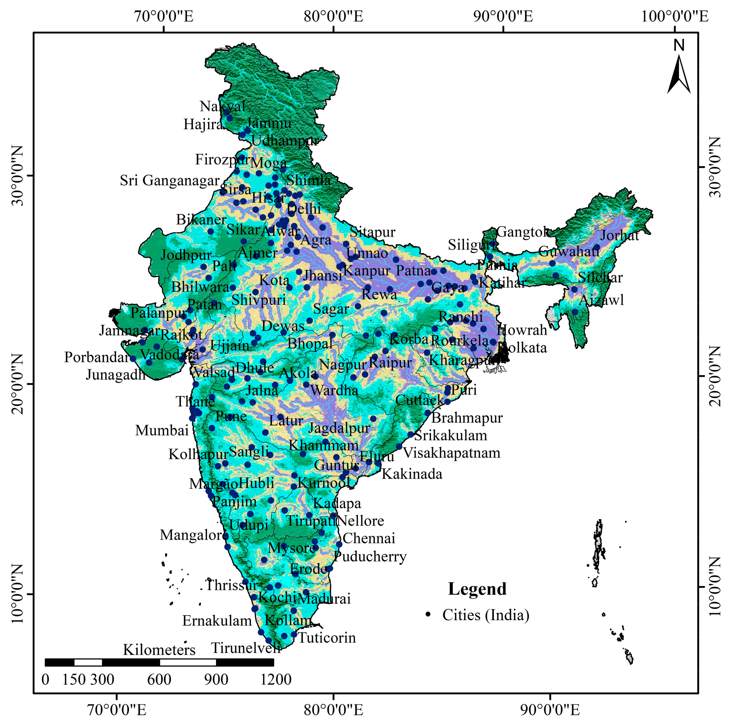
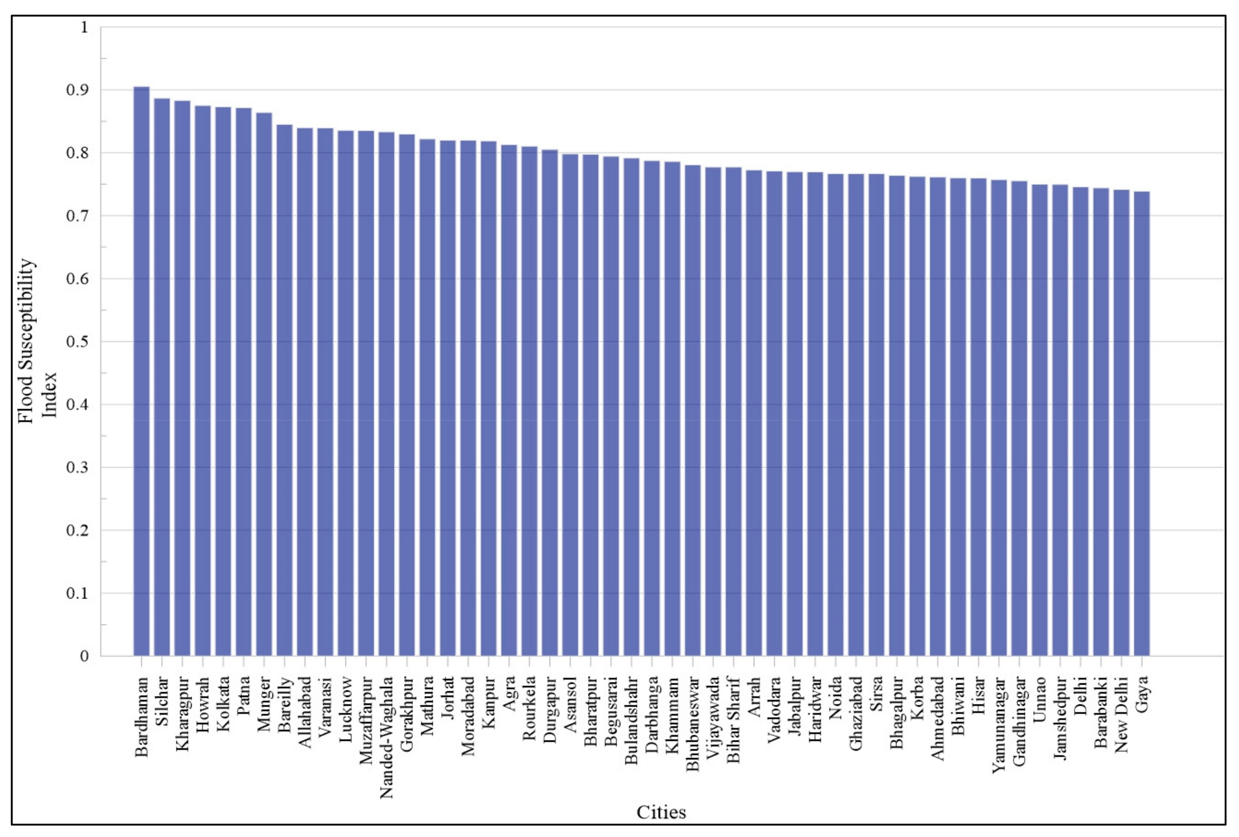
3.5. RFS Assessment of Indian Cities

The study reveals that a total of 54 cities (26.87%) fell into the high susceptibility zone, while 61 cities (30.35%) were categorized as moderate susceptibility areas. Additionally, 57 cities (28.36%) were in low susceptibility zones, with 29 cities (14.43%) falling outside susceptibility zones (Figure 13, Figure 14 and Figure 15). Notably, many cities within the high susceptibility zone were located in the Ganga and Brahmaputra basins. The top 10 most susceptible cities included Bardhaman, Silchar, Kharagpur, Howrah, Kolkata, Patna, Munger, Bareilly, Allahabad, and Varanasi Varanasi, each assigned RFS Indices ranging from 0.84 to 0.91 (Table S3). Furthermore, an analysis of Table S3 aided in identifying the cities that experienced the highest influence of each factor related to riverine floods. This analysis identified cities like Guwahati, Sri Ganganagar, Jagdalpur, Madurai, Burhanpur, Mathura, Bhiwani, Nellore, Panjim, and 43 others with a very high proximity to rivers. Additionally, 29 cities were found to be situated in areas characterized by very high drainage density. For cities with the highest drainage density, the list included Patna, Ellenabad, Sirsha, Agra, Bihar Sharif, Arrah, Bharatpur, Mathura, Kanpur, Aligarh, Bardhaman, Johrat, Unnao, and Begusarai, arranged in decreasing order. Regarding rainfall, Shillong, with 4185 mm, Udupi with 4163 mm, and Mangalore with 4051 mm, were the top three cities in India with the highest precipitation levels. Furthermore, cities situated in the Ganga, Brahmaputra, parts of the Indus basins, and the eastern coastline were found to have very low slope characteristics (<0.14°) (Table 6). Additionally, cities such as Gangtok, Shillong, Junagarh, and Tirupati exhibited high SPI, while Udhampur, Nakyal, Shillong, Shimla, Wanparti, and five other cities had high STI.

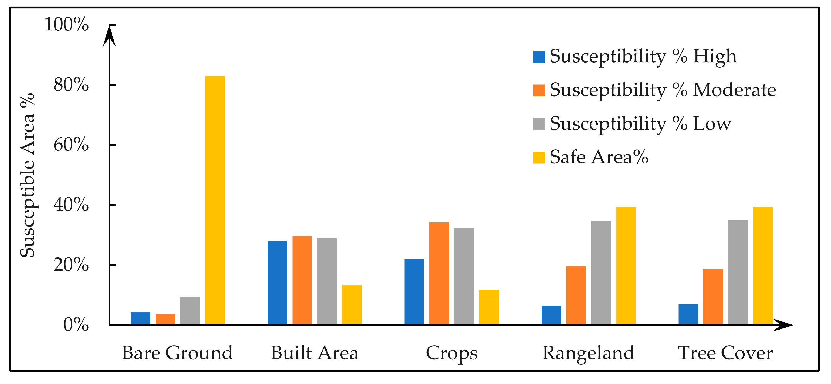
3.6. Land Cover Susceptibility Assessment of India

Conducting an RFS assessment of India’s land cover is essential for comprehensive land use planning. This assessment involved tabulating the areas of various land cover types within different susceptibility zones, utilizing RFS and LULC maps of India within ArcGIS.
The land cover categories include built area, crops, tree cover, rangeland, and bare ground, spanning 134,728 km2, 1,529,420 km2, 497,496 km2, 657,368 km2, and 141,268 km2, respectively. Within the total built area of India, 37,896 km2 (28.13%), 39,868 km2 (29.59%), 39,080 km2 (29.01%), and 17,884 km2 (13.27%) fell into high, moderate, low, and non-susceptible zones, respectively. Similarly, for the crop cover, 334,492 km2 (21.87%), 522,928 km2 (34.19%), 492,880 km2 (32.23%), and 179,120 km2 (11.71%) were categorized as high, moderate, low, and non-susceptible zones, respectively. In the case of tree cover, 34,424 km2 (6.92%), 93,232 km2 (18.74%), 173,556 km2 (34.89%), and 196,284 km2 (39.45%) were distributed among high, moderate, low, and non-susceptible zones, respectively. For rangeland, 42,304 km2 (6.44%), 128,552 km2 (19.56%), 227,416 km2 (34.59%), and 259,096 km2 (39.41%) were found in high, moderate, low, and non-susceptible zones, respectively. As for bare ground, 5916 km2 (4.19%), 4936 km2 (3.49%), 13,304 km2 (9.42%), and 117,108 km2 (82.90%) were allocated to high, moderate, low, and non-susceptible zones, respectively. Table 7 and Figure S2 depict the area of each land cover category in different RFS zones, while Table S4 and Figure 16 represent the same in percent. Agriculture has historically played a vital role in the Indian economy, but its performance has often been criticized for yielding low output. This study reveals that agricultural fields cover the largest portion of the total flood-susceptible area, followed by rangeland and tree cover. Focusing on production in low- and non-susceptible areas could significantly boost India’s economy. Furthermore, the study highlights that over 40% of the built-up area in India lies within flood-susceptible zones, with approximately 18,000 km2 falling into highly or moderately susceptible categories.

4. Discussion

The evaluation of susceptibility to riverine flooding at the national level and at the level of basins, cities, and across the land cover categories is a critical tool for making well-informed decisions, mitigating risks, enhancing emergency preparedness, strategizing infrastructure development, managing land usage, adapting to climate change, facilitating insurance protocols, and promoting ecological preservation.
This research conducted an analysis to examine the impact of several factors associated with RFS in India. Understanding the impact of numerous factors on riverine floods is of utmost significance, as it serves to mitigate the deleterious consequences of floods on both populations and the environment [93]. The FAHP was used to evaluate these parameters, resulting in an accuracy rate of 80.2% on the AUROC curve. The assessments provide a comprehensive understanding of flood susceptibility, enabling the implementation of effective strategies to protect human lives, assets, and ecosystems in flood-prone regions. Similar to previous studies by [94,95], the selection, assessment, and ranking of RFS influencing factors and their classes were conducted with the contribution of GDM. The study focused on macro- and meso-level RFS, RFS in cities, and land cover RFS. According to [52], the Ganga and Brahmaputra basins face the highest flood risk in the Indian subcontinent due to their high population density. However, the current study reveals that the Ganga, Godavari, and Brahmaputra basins cover the largest area under high RFS zones. Specifically, the area between the Godavari and Krishna basins, the Ganga basin, and the Subarnarekha basin has the highest percentage of their basin area categorized as high RFS zones. Additionally, our study assessed RFS in 201 cities and analyzed land cover in India using GIS techniques, which are essential for improved urban planning, flood management, and land use planning across the country.
The NRSC of ISRO recently published the Flood Affected Area Atlas of India in March 2023. It created a flood map of India and its states by processing historical satellite images from 1998 to 2022, identifying areas affected by past flood events and potential riverine flood zones where floods have not occurred in the past. However, the present study goes further by identifying high, moderate, low, and no riverine flood potential zones within India at the macroscale and in the Indian river basins at the mesoscale. The implementation of state-level planning, which is informed by individual state research, has resulted in interstate conflicts over river water resources in India, hence impeding the progress of holistic development. Hence, it is essential to implement basin-level planning that is centrally undertaken and informed by comprehensive basin-level investigations in order to mitigate the impact of floods and effectively manage water resources [96]. Consequently, our study focuses on Indian basins rather than Indian states.
The results of this study will provide significant insights for flood hazard managers and researchers in their selection of the GIS-based F-AHP approach for modeling RFS, conducting multilevel planning, urban planning, and land use planning. However, like any scientific endeavour, it has its limitations. Firstly, data availability and quality can be a challenge, as accurate and up-to-date information on basin morphology, rainfall patterns, and land-use changes may be lacking and distorted, especially on a large scale and in remote or poorly monitored areas. Secondly, the model’s effectiveness heavily depends on the accuracy of the input parameters and the choice of criteria, which can be subjective and influenced by the GDM’s judgment. Moreover, these models often assume static conditions, not accounting for evolving climate change impacts and socioeconomic dynamics. Thirdly, the spatial resolution of geospatial data can limit the precision of flood susceptibility assessments, especially in areas with complex topographies. Additionally, the model’s complexity may hinder its accessibility and usability for policymakers and local communities. Lastly, there is a need for validation and calibration against real-world flood events to assess the model’s accuracy and reliability, which entirely depend on the availability of accurate and well spatially distributed historical data. Addressing these limitations is crucial for enhancing the applicability and robustness of such flood susceptibility assessments. Moreover, it is important to acknowledge a notable constraint of the used methodology, as well as the broader practice of flood susceptibility mapping, which is the lack of capability to provide insights into flood depth or velocity. In order to enhance the comprehensiveness of future studies, it is recommended to integrate hydraulic modeling techniques, such as the advanced Hydrologic Engineering Center’s River Analysis System (HEC-RAS 5 and subsequent iterations). This software has the capability to produce two-dimensional maps depicting both depth and velocity.

5. Conclusions

The use of the integrated geographic MCDM model in this study facilitates the generation of precise RFS maps, hence enhancing the understanding of floods among many stakeholders, particularly decision-makers and the general public. This has the potential to enhance both mitigation and adaptation efforts. The objective of this research was to investigate the factors contributing to flooding in river basins, land cover, and urban areas in India. Additionally, a spatial model was constructed to assess the susceptibility to floods using MCDM and GIS. The investigation meticulously evaluated 14 factors, taking into consideration their association with floods. The FAHP model demonstrated that floods were primarily influenced by rainfall, drainage density, and proximity to streams. The river basins of the Ganga, Brahmaputra, and Godavari exhibited a high degree of vulnerability to flood risks. Conversely, some regions within the northern Indus basin, Luni basin, and western areas on the leeward side of the Western Ghats had lower susceptibility, with fewer occurrences of flood hazards. The geographical positioning of a majority of cities indicated a high susceptibility to flood hazards. Furthermore, the most flood-prone land use category was occupied by built-up and agricultural areas. Riverine floods have been shown to have significant impacts on both the structural and financial aspects of a country; however, it is worth noting that there may be some positive effects on farmers’ economies.
It is imperative that more investment be made by the government and relevant stakeholders in the domains of agriculture, land use, and urban planning. In order to facilitate the smooth flow of rainfall, it is recommended that new projects be situated at a considerable distance from streams and equipped with well-maintained drainage systems. It is important for residents to acquire knowledge of the causes and strategies for mitigating floods. Additionally, in order to improve on the findings of this study, it is recommended that future research endeavors include GIS in conjunction with emerging machine learning methodologies.

Supplementary Materials

The following supporting information can be downloaded at: https://www.mdpi.com/article/10.3390/w15223918/s1, Figure S1: Riverine Flood Susceptible Zones of Indian River Basins (in km2); Figure S2: Land Cover Area (in km2) in RFS Zones; Table S1: Ranks for the Classes of Conditioning Factors; Table S2: Pair-wise Comparison Matrix (FAHP); Table S3: Flood Susceptibility of the cities of India and their relation to major factors; Table S4: Land Cover Area (in %) in RFS Zones.

Author Contributions

Conceptualization, M.K. and R.K.; methodology, A.T., S.I.M. and S.B.; software, S.I.M., A.T. and S.B.; investigation, S.B.; validation, N.S.; data curation, R.K., A.T. and S.I.M.; resources, M.K. and N.S.; formal analysis, R.K., M.K., A.T., S.I.M. and S.B.; writing—original draft preparation, R.K., A.T., S.B., S.I.M. and M.K.; writing—review and editing, R.K., A.T., S.I.M., S.B., R.A. and M.K.; visualization, N.S.; supervision, N.S. and M.K.; project administration, M.K.; funding acquisition, R.A. All authors have read and agreed to the published version of the manuscript.

Funding

This research was partially funded by Grant-in-Aid for Scientific Research (c), grant number 21K05664 and Sumitomo Foundation grant number 2330169.

Data Availability Statement

All data generated or analyzed during the study are included in this published article.

Acknowledgments

The authors express their gratitude to the Department of Geography at the Central University of Haryana, Mahendragarh, India, for providing a technically robust platform, supporting software services (ArcGIS 10.8 and SPSS 26.0), and a supportive atmosphere for the successful execution of this research.

Conflicts of Interest

The authors unanimously declare that there are no conflict of interest to declare.

References

  1. Lee, S.; Kim, J.-C.; Jung, H.-S.; Lee, M.J.; Lee, S. Spatial prediction of flood susceptibility using random-forest and boosted-tree models in Seoul metropolitan city, Korea. Geomat. Nat. Hazards Risk 2017, 8, 1185–1203. [Google Scholar] [CrossRef]
  2. Ahmadlou, M.; Al-Fugara, A.; Al-Shabeeb, A.R.; Arora, A.; Al-Adamat, R.; Pham, Q.B.; Al-Ansari, N.; Linh, N.T.T.; Sajedi, H. Flood susceptibility mapping and assessment using a novel deep learning model combining multilayer perceptron and autoencoder neural networks. J. Flood Risk Manag. 2020, 14, e12683. [Google Scholar] [CrossRef]
  3. Diaz, J.H. Global Climate Changes, Natural Disasters, and Travel Health Risks. J. Travel Med. 2006, 13, 361–372. [Google Scholar] [CrossRef]
  4. Zêzere, J.L.; Pereira, S.; Tavares, A.O.; Bateira, C.; Trigo, R.M.; Quaresma, I.; Santos, P.P.; Santos, M.; Verde, J. DISASTER: A GIS database on hydro-geomorphologic disasters in Portugal. Nat. Hazards 2014, 72, 503–532. [Google Scholar] [CrossRef]
  5. He, B.; Huang, X.; Ma, M.; Chang, Q.; Tu, Y.; Li, Q.; Zhang, K.; Hong, Y. Analysis of flash flood disaster characteristics in China from 2011 to 2015. Nat. Hazards 2017, 90, 407–420. [Google Scholar] [CrossRef]
  6. Kundzewicz, Z.W.; Su, B.; Wang, Y.; Wang, G.; Wang, G.; Huang, J.; Jiang, T. Flood risk in a range of spatial perspectives—From global to local scales. Nat. Hazards Earth Syst. Sci. 2019, 19, 1319–1328. [Google Scholar] [CrossRef]
  7. Merz, B.; Blöschl, G.; Vorogushyn, S.; Dottori, F.; Aerts, J.C.J.H.; Bates, P.; Bertola, M.; Kemter, M.; Kreibich, H.; Lall, U.; et al. Causes, impacts and patterns of disastrous river floods. Nat. Rev. Earth Environ. 2021, 2, 592–609. [Google Scholar] [CrossRef]
  8. Purohit, J.; Rout, H.S. Impact of climate change on human health concerning climate-induced natural disaster: Evidence from an eastern Indian state. Clim. Chang. 2023, 176, 1–22. [Google Scholar] [CrossRef]
  9. Sanchez, M.C.J. World Disasters Report 2020: Chapter 4 Reducing Risks and Building Resilience–Minimizing the Impacts of Potential and Predicted Extreme Events. International Federation of Red Cross and Red Crescent Societies. 2020. Available online: https://research.utwente.nl/en/publications/world-disasters-report-2020-chapter-4-reducing-risks-and-building (accessed on 27 September 2023).
  10. Haynes, K.; Coates, L.; Honert, R.v.D.; Gissing, A.; Bird, D.; de Oliveira, F.D.; Darcy, R.; Smith, C.; Radford, D. Exploring the circumstances surrounding flood fatalities in Australia—1900–2015 and the implications for policy and practice. Environ. Sci. Policy 2017, 76, 165–176. [Google Scholar] [CrossRef]
  11. Jamali, B.; Bach, P.M.; Deletic, A. Rainwater harvesting for urban flood management–An integrated modelling framework. Water Res. 2019, 171, 115372. [Google Scholar] [CrossRef] [PubMed]
  12. Raj, R.; Yunus, A.P.; Pani, P.; Avtar, R. Towards evaluating gully erosion volume and erosion rates in the Chambal badlands, Central India. Land Degrad. Dev. 2022, 33, 1495–1510. [Google Scholar] [CrossRef]
  13. Saini, A.; Sahu, N.; Kumar, P.; Nayak, S.; Duan, W.; Avtar, R.; Behera, S. Advanced Rainfall Trend Analysis of 117 Years over West Coast Plain and Hill Agro-Climatic Region of India. Atmosphere 2020, 11, 1225. [Google Scholar] [CrossRef]
  14. Doswell, C.A.; Brooks, H.E.; Maddox, R.A. Flash Flood Forecasting: An Ingredients-Based Methodology. Weather Forecast. 1996, 11, 560–581. [Google Scholar] [CrossRef]
  15. Sahu, N.; Panda, A.; Nayak, S.; Saini, A.; Mishra, M.; Sayama, T.; Sahu, L.; Duan, W.; Avtar, R.; Behera, S. Impact of Indo-Pacific Climate Variability on High Streamflow Events in Mahanadi River Basin, India. Water 2020, 12, 1952. [Google Scholar] [CrossRef]
  16. Mohanty, M.P.; Mudgil, S.; Karmakar, S. Flood management in India: A focussed review on the current status and future challenges. Int. J. Disaster Risk Reduct. 2020, 49, 101660. [Google Scholar] [CrossRef]
  17. Manivannan, S.; Thilagam, V.K.; Khola, O. Soil and water conservation in India: Strategies and research challenges. J. Soil Water Conserv. 2017, 16, 312. [Google Scholar] [CrossRef]
  18. Bhawan, S.; Puram, R. Watershed Atlas of India. New Delhi Center Water Commision, 2014. Available online: https://www.researchgate.net/publication/316663108_WATERSHED_ATLAS_OF_INDIA (accessed on 24 September 2023).
  19. Sutradhar, S.; Mondal, P. Prioritization of watersheds based on morphometric assessment in relation to flood management: A case study of Ajay river basin, Eastern India. Watershed Ecol. Environ. 2023, 5, 1–11. [Google Scholar] [CrossRef]
  20. Panda, P.K. Vulnerability of flood in India: A remote sensing and GIS approach for warning, mitigation and management. Asian J. Sci. Technol. 2014, 5, 843–846. [Google Scholar]
  21. Green, C. Flood Risk Management in Europe: The Flood Problem and Interventions; Revision 4; STAR-FLOOD Consortium: Utrecht, The Netherlands, 2013. [Google Scholar]
  22. Conitz, F.; Zingraff-Hamed, A.; Lupp, G.; Pauleit, S. Non-Structural Flood Management in European Rural Mountain Areas—Are Scientists Supporting Implementation? Hydrology 2021, 8, 167. [Google Scholar] [CrossRef]
  23. Kron, W.; Steuer, M.; Löw, P.; Wirtz, A. How to deal properly with a natural catastrophe database—Analysis of flood losses. Nat. Hazards Earth Syst. Sci. 2012, 12, 535–550. [Google Scholar] [CrossRef]
  24. Nied, M.; Schröter, K.; Lüdtke, S.; Nguyen, V.D.; Merz, B. What are the hydro-meteorological controls on flood characteristics? J. Hydrol. 2017, 545, 310–326. [Google Scholar] [CrossRef]
  25. Youssef, A.M.; Pradhan, B.; Sefry, S.A. Flash flood susceptibility assessment in Jeddah city (Kingdom of Saudi Arabia) using bivariate and multivariate statistical models. Environ. Earth Sci. 2015, 75, 1–16. [Google Scholar] [CrossRef]
  26. Jothibasu, A.; Anbazhagan, S. Flood susceptibility appraisal in Ponnaiyar River Basin, India using frequency ratio (FR) and Shannon’s Entropy (SE) models. Int. J. Adv. Rem. Sens. GIS 2016, 5, 1946–1962. [Google Scholar]
  27. Rehman, S.; Hasan, M.S.U.; Rai, A.K.; Rahaman, M.H.; Avtar, R.; Sajjad, H. Integrated approach for spatial flood susceptibility assessment in Bhagirathi sub-basin, India using entropy information theory and geospatial technology. Risk Anal. 2022, 42, 2765–2780. [Google Scholar]
  28. Rahmati, O.; Pourghasemi, H.R.; Zeinivand, H. Flood susceptibility mapping using frequency ratio and weights-of-evidence models in the Golastan Province, Iran. Geocarto Int. 2015, 31, 42–70. [Google Scholar] [CrossRef]
  29. Zhao, G.; Pang, B.; Xu, Z.; Peng, D.; Xu, L. Assessment of urban flood susceptibility using semi-supervised machine learning model. Sci. Total Environ. 2018, 659, 940–949. [Google Scholar] [CrossRef]
  30. Chen, J.; Zhang, Y.; Chen, Z.; Nie, Z. Improving assessment of groundwater sustainability with analytic hierarchy process and information entropy method: A case study of the Hohhot Plain, China. Environ. Earth Sci. 2014, 73, 2353–2363. [Google Scholar] [CrossRef]
  31. Li, J. A data-driven improved fuzzy logic control optimization-simulation tool for reducing flooding volume at downstream urban drainage systems. Sci. Total Environ. 2020, 732, 138931. [Google Scholar] [CrossRef]
  32. Tien Bui, D.; Khosravi, K.; Shahabi, H.; Daggupati, P.; Adamowski, J.F.; Melesse, A.M.; Pham, B.T.; Pourghasemi, H.R.; Bahrami, S. Flood Spatial Modeling in Northern Iran Using Remote Sensing and GIS: A Comparison between Evidential Belief Functions and Its Ensemble with a Multivariate Logistic Regression Model. Remote Sens. 2019, 11, 1589. [Google Scholar] [CrossRef]
  33. Tiwari, M.K.; Chatterjee, C. Development of an accurate and reliable hourly flood forecasting model using wavelet–bootstrap–ANN (WBANN) hybrid approach. J. Hydrol. 2010, 394, 458–470. [Google Scholar] [CrossRef]
  34. Kia, M.B.; Pirasteh, S.; Pradhan, B.; Mahmud, A.R.; Sulaiman, W.N.A.; Moradi, A. An artificial neural network model for flood simulation using GIS: Johor River Basin, Malaysia. Environ. Earth Sci. 2011, 67, 251–264. [Google Scholar] [CrossRef]
  35. Elsafi, S.H. Artificial Neural Networks (ANNs) for flood forecasting at Dongola Station in the River Nile, Sudan. Alex. Eng. J. 2014, 53, 655–662. [Google Scholar] [CrossRef]
  36. Kourgialas, N.N.; Anyfanti, I.; Karatzas, G.P.; Dokou, Z. An integrated method for assessing drought prone areas–Water efficiency practices for a climate resilient Mediterranean agriculture. Sci. Total Environ. 2018, 625, 1290–1300. [Google Scholar] [CrossRef] [PubMed]
  37. Khosravi, K.; Pham, B.T.; Chapi, K.; Shirzadi, A.; Shahabi, H.; Revhaug, I.; Prakash, I.; Bui, D.T. A comparative assessment of decision trees algorithms for flash flood susceptibility modeling at Haraz watershed, northern Iran. Sci. Total Environ. 2018, 627, 744–755. [Google Scholar] [CrossRef]
  38. Tehrany, M.S.; Pradhan, B.; Mansor, S.; Ahmad, N. Flood susceptibility assessment using GIS-based support vector machine model with different kernel types. CATENA 2015, 125, 91–101. [Google Scholar] [CrossRef]
  39. Choubin, B.; Moradi, E.; Golshan, M.; Adamowski, J.; Sajedi-Hosseini, F.; Mosavi, A. An ensemble prediction of flood susceptibility using multivariate discriminant analysis, classification and regression trees, and support vector machines. Sci. Total Environ. 2018, 651, 2087–2096. [Google Scholar] [CrossRef]
  40. Termeh, S.V.R.; Kornejady, A.; Pourghasemi, H.R.; Keesstra, S. Flood susceptibility mapping using novel ensembles of adaptive neuro fuzzy inference system and metaheuristic algorithms. Sci. Total Environ. 2018, 615, 438–451. [Google Scholar] [CrossRef]
  41. Amodei, D.; Olah, C.; Steinhardt, J.; Christiano, P.; Schulman, J.; Mané, D. Concrete Problems in AI Safety. arXiv 2016, arXiv:1606.06565. [Google Scholar] [CrossRef]
  42. Poursabzi-Sangdeh, F.; Goldstein, D.G.; Hofman, J.M.; Vaughan, J.W.W.; Wallach, H. Manipulating and Measuring Model Interpretability. In Proceedings of the CHI’21: CHI Conference on Human Factors in Computing Systems, Yokohama, Japan, 8–13 May 2021. [Google Scholar]
  43. Murdoch, W.J.; Singh, C.; Kumbier, K.; Abbasi-Asl, R.; Yu, B. Definitions, methods, and applications in interpretable machine learning. Proc. Natl. Acad. Sci. USA 2019, 116, 22071–22080. [Google Scholar] [CrossRef]
  44. Saaty, T.L.; Tran, L.T. On the invalidity of fuzzifying numerical judgments in the Analytic Hierarchy Process. Math. Comput. Model. 2007, 46, 962–975. [Google Scholar] [CrossRef]
  45. Saaty, T.L. The Analytic Hierarchy Process; McGraw-Hill: New York, NY, USA, 1980. [Google Scholar]
  46. Kahraman, C.; Ruan, D.; Doǧan, I. Fuzzy group decision-making for facility location selection. Inf. Sci. 2003, 157, 135–153. [Google Scholar] [CrossRef]
  47. Das, B.; Pal, S.C. Combination of GIS and fuzzy-AHP for delineating groundwater recharge potential zones in the critical Goghat-II block of West Bengal, India. HydroResearch 2019, 2, 21–30. [Google Scholar] [CrossRef]
  48. van Laarhoven, P.; Pedrycz, W. A fuzzy extension of Saaty’s priority theory. Fuzzy Sets Syst. 1983, 11, 229–241. [Google Scholar] [CrossRef]
  49. Kubler, S.; Robert, J.; Derigent, W.; Voisin, A.; Le Traon, Y. A state-of the-art survey & testbed of fuzzy AHP (FAHP) applications. Expert Syst. Appl. 2016, 65, 398–422. [Google Scholar] [CrossRef]
  50. Panda, D.K.; Tiwari, V.M.; Rodell, M. Groundwater Variability Across India, Under Contrasting Human and Natural Conditions. Earth’s Future 2022, 10, 2513. [Google Scholar] [CrossRef]
  51. United Nations Department of Economic and Social Affairs. Population Division, World Population Prospects 2022: Summary of Results. UN DESA/POP/2022/TR/NO. 3. 2022. Available online: https://desapublications.un.org/file/989/download (accessed on 24 September 2023).
  52. Vegad, U.; Pokhrel, Y.; Mishra, V.; Ghosh, A.; Kar, S.K. Application of analytical hierarchy process (AHP) for flood risk assessment: A case study in Malda district of West Bengal, India. Hydrol. Earth Syst. Sci. Discuss. 2018, 94, 349–368. [Google Scholar]
  53. Ganio, L.M.; Torgersen, C.E.; Gresswell, R.E. A geostatistical approach for describing spatial pattern in stream networks. Front. Ecol. Environ. 2005, 3, 138–144. [Google Scholar] [CrossRef]
  54. Horton, R.E. Erosional development of streams and their drainage basins; hydrophysical approach to quantitative morphology. Geol. Soc. Am. Bull. 1945, 56, 275–370. [Google Scholar] [CrossRef]
  55. Wolock, D.M.; McCabe, G.J., Jr. Comparison of single and multiple flow direction algorithms for computing topo-graphic parameters in TOPMODEL. Water Resour. Res. 1995, 31, 1315–1324. [Google Scholar] [CrossRef]
  56. Yin, J.; Guo, S.; Liu, Z.; Yang, G.; Zhong, Y.; Liu, D. Uncertainty analysis of bivariate design flood estimation and its im-pacts on reservoir routing. Water Resour. Manag. 2018, 32, 1795–1809. [Google Scholar] [CrossRef]
  57. Jenks, G.F. Optimal Data Classification for Choropleth Maps. Dep. Geogr. Univ. Kans. Occas. Pap. 1977. Available online: https://cir.nii.ac.jp/crid/1570572700325134464 (accessed on 5 October 2023).
  58. Campbell, J.B.; Wynne, R.H. Introduction to Remote Sensing; Guilford Press: New York, NY, USA, 2011. [Google Scholar]
  59. Tehrany, M.S.; Kumar, L. The application of a Dempster–Shafer-based evidential belief function in flood susceptibility mapping and comparison with frequency ratio and logistic regression methods. Environ. Earth Sci. 2018, 77, 490. [Google Scholar] [CrossRef]
  60. Kaliraj, S.; Chandrasekar, N.; Magesh, N. Morphometric analysis of the River Thamirabarani sub-basin in Kanya-kumari District, South west coast of Tamil Nadu, India, using remote sensing and GIS. Environ. Earth Sci. 2015, 73, 7375–7401. [Google Scholar] [CrossRef]
  61. Mousavi, S.M.; Ataie-Ashtiani, B.; Hosseini, S.M. Comparison of statistical and mcdm approaches for flood susceptibility mapping in northern Iran. J. Hydrol. 2022, 612, 128072. [Google Scholar] [CrossRef]
  62. Ohlmacher, G.C. Plan curvature and landslide probability in regions dominated by earth flows and earth slides. Eng. Geol. 2007, 91, 117–134. [Google Scholar] [CrossRef]
  63. Mahmoud, S.H.; Gan, T.Y. Urbanization and climate change implications in flood risk management: Developing an efficient decision support system for flood susceptibility mapping. Sci. Total Environ. 2018, 636, 152–167. [Google Scholar] [CrossRef] [PubMed]
  64. Domeneghetti, A.; Tarpanelli, A.; Brocca, L.; Barbetta, S.; Moramarco, T.; Castellarin, A.; Brath, A. The use of remote sensing-derived water surface data for hydraulic model calibration. Remote Sens. Environ. 2014, 149, 130–141. [Google Scholar] [CrossRef]
  65. Montgomery, D.R.; Dietrich, W.E. Source areas, drainage density, and channel initiation. Water Resour. Res. 1989, 25, 1907–1918. [Google Scholar] [CrossRef]
  66. Abu El-Magd, S.A.; Orabi, H.O.; Ali, S.A.; Parvin, F.; Pham, Q.B. An integrated approach for evaluating the flash flood risk and potential erosion using the hydrologic indices and morpho-tectonic parameters. Environ. Earth Sci. 2021, 80, 694. [Google Scholar] [CrossRef]
  67. Wicks, J.; Bathurst, J. SHESED: A physically based, distributed erosion and sediment yield component for the SHE hydrological modelling system. J. Hydrol. 1996, 175, 213–238. [Google Scholar] [CrossRef]
  68. Graham, D.J.; Rollet, A.; Piégay, H.; Rice, S.P. Maximizing the accuracy of image-based surface sediment sampling techniques. Water Resour. Res. 2010, 46, 6940. [Google Scholar] [CrossRef]
  69. Beven, K.J.; Kirkby, M.J. A physically based, variable contributing area model of basin hydrology/Un modèle à base physique de zone d’appel variable de l’hydrologie du bassin versant. Hydrol. Sci. J. 1979, 24, 43–69. [Google Scholar] [CrossRef]
  70. Nandi, A.; Mandal, A.; Wilson, M.; Smith, D. Flood hazard mapping in Jamaica using principal component analysis and logistic regression. Environ. Earth Sci. 2016, 75, 465. [Google Scholar] [CrossRef]
  71. Anni, A.H.; Cohen, S.; Praskievicz, S. Sensitivity of urban flood simulations to stormwater infrastructure and soil in-filtration. J. Hydrol. 2020, 588, 125028. [Google Scholar] [CrossRef]
  72. Sugianto, S.; Deli, A.; Miswar, E.; Rusdi, M.; Irham, M. The Effect of Land Use and Land Cover Changes on Flood Occurrence in Teunom Watershed, Aceh Jaya. Land 2022, 11, 1271. [Google Scholar] [CrossRef]
  73. Budyko, M.I. Climate and Life; Academic Press: Cambridge, MA, USA, 1974. [Google Scholar]
  74. Eriyagama, N.; Thilakarathne, M.; Tharuka, P.; Munaweera, T.; Muthuwatta, L.; Smakhtin, V.; Premachandra, W.W.; Pindeniya, D.; Wijayarathne, N.S.; Udamulla, L. Actual and perceived causes of flood risk: Climate versus anthropogenic effects in a wet zone catchment in Sri Lanka. Water Int. 2017, 42, 874–892. [Google Scholar] [CrossRef]
  75. Arnold, C.L., Jr.; Gibbons, C.J. Impervious Surface Coverage: The Emergence of a Key Environmental Indicator. J. Am. Plan. Assoc. 1996, 62, 243–258. [Google Scholar] [CrossRef]
  76. AghaKouchak, A.; Feldman, D.; Hoerling, M.; Huxman, T.; Lund, J. Water and climate: Recognize anthropogenic drought. Nature 2015, 524, 409–411. [Google Scholar] [CrossRef]
  77. Ghosh, S.; Saha, S.; Bera, B. Flood susceptibility zonation using advanced ensemble machine learning models within Himalayan foreland basin. Nat. Hazards Res. 2022, 2, 363–374. [Google Scholar] [CrossRef]
  78. Merz, B.; Thieken, A.; Gocht, M. Flood Risk Mapping at The Local Scale: Concepts and Challenges. In Landslides in Sensitive Clays; Springer Science and Business Media LLC: New York, NY, USA, 2007; pp. 231–251. [Google Scholar]
  79. Handfield, R.; Walton, S.V.; Sroufe, R.; Melnyk, S.A. Applying environmental criteria to supplier assessment: A study in the application of the Analytical Hierarchy Process. Eur. J. Oper. Res. 2002, 141, 70–87. [Google Scholar] [CrossRef]
  80. Spanidis, P.-M.; Roumpos, C.; Pavloudakis, F. A fuzzy-AHP methodology for Planning the risk management of Natural hazards in surface mining projects. Sustainability 2021, 13, 2369. [Google Scholar] [CrossRef]
  81. Calantone, R.J.; Benedetto, C.A.; Schmidt, J.B. Using the Analytic Hierarchy Process in New Product Screening. J. Prod. Innov. Manag. 1999, 16, 65–76. [Google Scholar] [CrossRef]
  82. Zadeh, L.A. Fuzzy sets. Inf. Control 1965, 8, 338–353. [Google Scholar] [CrossRef]
  83. Do, Q.H.; Chen, J.-F.; Hsieh, H.-N. Trapezoidal fuzzy AHP and fuzzy comprehensive evaluation approaches for evaluating academic library service. WSEAS Trans. Comput. 2015, 14, 607–619. [Google Scholar]
  84. Herrera-Viedma, E.; Pasi, G.; Lopez-Herrera, A.G.; Porcel, C. Evaluating the information quality of web sites: A methodology based on fuzzy computing with words. J. Am. Soc. Inf. Sci. Technol. 2006, 57, 538–549. [Google Scholar] [CrossRef]
  85. Kannan, D.; Khodaverdi, R.; Olfat, L.; Jafarian, A.; Diabat, A. Integrated fuzzy multi criteria decision making method and multi-objective programming approach for supplier selection and order allocation in a green supply chain. J. Clean. Prod. 2013, 47, 355–367. [Google Scholar] [CrossRef]
  86. Esmaeili, A.; Kahnali, R.A.; Rostamzadeh, R.; Kazimieras, E.; Sepahvand, A. The Formulation of Organizational Strategies Through Integration of Freeman Model, Swot, and Fuzzy Mcdm Methods: A Case Study of Oil Industry. Transform. Bus. Econ. 2014, 13, 602–627. [Google Scholar]
  87. Chen, H.; Wood, M.D.; Linstead, C.; Maltby, E. Uncertainty analysis in a GIS-based multi-criteria analysis tool for river catchment management. Environ. Model. Softw. 2011, 26, 395–405. [Google Scholar] [CrossRef]
  88. Moslem, S.; Ghorbanzadeh, O.; Blaschke, T.; Duleba, S. Analysing Stakeholder Consensus for a Sustainable Transport Development Decision by the Fuzzy AHP and Interval AHP. Sustainability 2019, 11, 3271. [Google Scholar] [CrossRef]
  89. Mallick, J.; Singh, R.K.; AlAwadh, M.A.; Islam, S.; Khan, R.A.; Qureshi, M.N. GIS-based landslide susceptibility evalua-tion using fuzzy-AHP multi-criteria decision-making techniques in the Abha Watershed, Saudi Arabia. Environ. Earth Sci. 2018, 77, 276. [Google Scholar] [CrossRef]
  90. Nachappa, T.G.; Piralilou, S.T.; Gholamnia, K.; Ghorbanzadeh, O.; Rahmati, O.; Blaschke, T. Flood susceptibility mapping with machine learning, multi-criteria decision analysis and ensemble using Dempster Shafer Theory. J. Hydrol. 2020, 590, 125275. [Google Scholar] [CrossRef]
  91. Tehrany, M.S.; Pradhan, B.; Jebur, M.N. Spatial prediction of flood susceptible areas using rule based decision tree (DT) and a novel ensemble bivariate and multivariate statistical models in GIS. J. Hydrol. 2013, 504, 69–79. [Google Scholar] [CrossRef]
  92. Yesilnacar, E.; Topal, T. Landslide susceptibility mapping: A comparison of logistic regression and neural networks methods in a medium scale study, Hendek region (Turkey). Eng. Geol. 2005, 79, 251–266. [Google Scholar] [CrossRef]
  93. Kundzewicz, Z.W.; Hegger, D.; Matczak, P.; Driessen, P. Flood-risk reduction: Structural measures and diverse strategies. Proc. Natl. Acad. Sci. USA 2018, 115, 12321–12325. [Google Scholar] [CrossRef]
  94. Ceccato, L.; Giannini, V.; Giupponi, C. Participatory assessment of adaptation strategies to flood risk in the Upper Brahmaputra and Danube river basins. Environ. Sci. Policy 2011, 14, 1163–1174. [Google Scholar] [CrossRef]
  95. Sarmah, T.; Das, S.; Narendr, A.; Aithal, B.H. Assessing human vulnerability to urban flood hazard using the analytic hierarchy process and geographic information system. Int. J. Disaster Risk Reduct. 2020, 50, 101659. [Google Scholar] [CrossRef]
  96. Gao, X.; Schlosser, C.A.; Fant, C.; Strzepek, K. The impact of climate change policy on the risk of water stress in southern and eastern Asia. Environ. Res. Lett. 2018, 13, 064039. [Google Scholar] [CrossRef]
Figure 1. Study Area: Indian river basins.
Water 15 03918 g001
Figure 2. Flow chart of methodology.
Water 15 03918 g002
Figure 3. Spatial database of conditioning factors; (a) distance from rivers, (b) drainage density, (c) elevation, (d) slope, (e) aspect, (f) plan curvature, (g) profile curvature, (h) SPI, (i) STI, (j) TWI, (k) soil texture, (l) mean annual rainfall, (m) lithology, (n) LULC.
Water 15 03918 g003aWater 15 03918 g003b
Figure 4. Triangular fuzzy number.
Water 15 03918 g004
Figure 5. Fuzzy linguistic terms [85].
Water 15 03918 g005
Figure 6. Influence of factors on riverine floods.
Water 15 03918 g006
Figure 7. RFS Map of India.
Water 15 03918 g007
Figure 8. Riverine flood susceptible area: India.
Water 15 03918 g008
Figure 9. Validation points.
Water 15 03918 g009
Figure 10. AUROC curve.
Water 15 03918 g010
Figure 11. RFS maps of Indian river basins; (a) Ganga Basin, (b) Indus Basin, (c) Brahamaputra Basin, (d) Godavari Basin, (e) Krishna Basin, (f) Cauvery Basin, (g) Narmada Basin, (h) Tapi Basin, (i) Mahanadi Basin, (j) Brahmani-Baitarni Basin, (k) Subarnarekha Basin, (l) Pennar Basin.
Water 15 03918 g011
Figure 12. Riverine flood-susceptible zones of Indian river basins (in km2).
Water 15 03918 g012
Figure 13. RFS Map of the Indian cities.
Water 15 03918 g013
Figure 14. Number of cities in RFS zones.
Water 15 03918 g014
Figure 15. RFS Index of 50 highly susceptible cities.
Water 15 03918 g015
Figure 16. Land cover area (in %) in RFS zones.
Water 15 03918 g016
Table 1. Specifications, relation, and method of data used in the study.
FactorsMap LayerResolution/ScalePreparation MethodRelation with
Flood Susceptibility
Data SourcePeriod
Hydrological FactorsProximity
to Rivers
30 m × 30 mMultiple ring bufferingPositive RelationSRTM Plus V3
(https://earthexplorer.usgs.gov/); accessed on 30 October 2022.
2013
Drainage DensitySpatial analysis using the line density tool
Geomorphological FactorsElevationDEM Classification
Spatial analysis using slope, aspect and curvature tools respectively
Negative Relation
Slope
AspectNorth Facing More Susceptible
and vice-versa
Plan CurvatureNegative Relation
Profile CurvaturePositive Relation
TWICalculating map algebra using raster calculator and Equations (1) and (2)
SPI
STI
Soil Texture1:5,000,000Clipped from World Soil Database. Sequence No. matched in attribute tableNegative RelationFAO (https://data.apps.fao.org/map/catalog/srv/eng/catalog.search#/metadata/cc45a270-88fd-11da-a88f-000d939bc5d8); accessed on 4 December 2022.1972
LithologyClipped from World Geology DatabaseUSGS WEP (https://pubs.er.usgs.gov/publication/ofr97470C); accessed on 7
November 2022.
1997
Meteorological FactorMean Annual Rainfall0.5° × 0.5°30 years gridded
data interpolation using IDW
Positive RelationCRU TS v. 4.07
(https://crudata.uea.ac.uk/cru/data/hrg/cru_ts_4.07/cruts.2304141047.v4.07/pre/); accessed on 22 March 2023.
1992–2022
Anthropogenic FactorLULC10 m × 10 mClipped from World LULC DatabaseSENTINEL 2A
(https://www.arcgis.com/home/item.html?id=d3da5dd386d140cf93fc9ecbf8da5e31); accessed on 10 November 2022.
2020
Ancillary DataIndia Outline1:1,000,000Downloaded and merged internal polygons SOI (https://onlinemaps.surveyofindia.gov.in/Digital_Product_Show.aspx); accessed on 30 October 2022.
Table 2. Triangular fuzzy numbers analytical conversion operations [85].
Saaty ScaleLinguistic TermsTriangular Fuzzy
Numbers Scale
Reversed ValuesTFN Conversion
1Equal (EQ)(1,1,1)1/1(1/1, 1/1, 1/1)
3Moderate (MD)(2,3,4)1/3(1/4, 1/3, 1/2)
5Strong (ST)(4,5,6)1/5(1/6, 1/5, 1/4)
7Very Strong (VS)(6,7,8)1/7(1/8, 1/7, 1/6)
9Extremely Strong (ES)(9,9,9)1/9(1/9, 1/9, 1/9)
2 (1,2,3)1/2(1/3, 1/2, 1/1)
4Intermediate Values(3,4,5)1/4(1/5, 1/4, 1/3)
6 (5,6,7)1/6(1/7, 1/6, 1/5)
8 (7,8,9)1/8(1/9, 1/8, 1/7)
Table 3. Random index values [45].
n3456789101112131415
RI0.580.901.121.241.321.411.451.511.521.541.561.581.59
Table 4. Rank of Factors.
FactorsRankInfluence
Distance from Rivers141.00
Drainage Density130.88
M. A. Rainfall 1992–2022120.75
Elevation110.63
Slope100.50
SPI90.38
STI90.38
Plan Curvature80.25
Profile Curvature80.25
Lithology70.13
LULC 202270.13
Soil Texture70.13
TWI70.13
Aspect60.00
Table 5. FAHP normalized weights.
FactorsGeometric MeanFuzzy WeightsNormalized Weights
Distance from Rivers4.084.935.740.23590.22840.21700.2271
Drainage Density3.414.144.910.19750.19180.18550.1916
Rainfall 1992–20222.813.414.100.16280.15800.15490.1586
Elevation1.171.591.990.06770.07380.07530.0722
Slope1.181.571.950.06820.07280.07390.0716
SPI1.011.291.670.05830.05970.06310.0604
STI1.011.291.670.05830.05970.06310.0604
Plan Curvature0.530.730.990.03070.03390.03720.0339
Profile Curvature0.520.720.970.03010.03330.03680.0334
Lithology0.390.480.610.02270.02210.02310.0226
LULC 20220.380.460.590.02180.02140.02250.0219
Soil Texture0.380.460.590.02180.02140.02250.0219
TWI0.230.290.380.01330.01340.01420.0136
Aspect0.190.220.290.01080.01040.01080.0107
Table 6. Basin-wise area of varied degrees of riverine flood-susceptible zones.
BASINSSusceptible Zones (in km2)Susceptible Area
(in km2)
Safe Area
(in km2)
Total Area
(in km2)
High Susceptible
Area %
HighModerateLow
Ganga Basin25,4296256,740179,304690,34086,968777,30832.71
Godavari Basin61,368106,19297,676265,23626,808292,04421.01
Krishna Basin10,31672,428119,496202,24041,728243,9684.23
Indus Basin16,13262,48893,304168,996263,280432,2763.73
Mahanadi Basin28,12446,48445,348119,95618,868138,82420.26
Brahmaputra Basin37,18437,34443,112117,64057,740175,38021.20
Kutch-Saurashtra-Luni Basin610031,47250,42487,99686,352174,3483.50
Narmada Basin853626,91245,59681,04410,88091,9249.29
WFR South of Tapi Basin65610,80058,25269,70842,432112,1400.58
Cauvery Basin198019,67639,79661,45216,77678,2282.53
Tapi Basin351215,34028,25247,10415,49662,6005.61
EFR bw Pennar and Cauvery Basin322819,90023,42446,55216,50063,0525.12
Brahmani and Baitarni Basin857220,57215,24444,388441648,80417.56
Pennar Basin296813,72020,12436,81217,76054,5725.44
Mahi Basin650012,12813,23231,860506036,92017.61
EFR South of Cauvery Basin112671223,87630,700714837,8480.30
Barak Basin4556755213,00825,11619,59644,71210.19
Subarnarekha Basin55049920872424,14890025,04821.97
Sabarmati Basin418012,252600022,432709229,52414.16
EFR bw Krishna and Pennar Basin348692813,04420,320421224,5321.42
EFR bw Mahanadi and Godavari Basins20363214,40018,05225,34043,3920.05
EFR bw Godavari and Krishna Basin3436404412876080760845.16
Myanmar Basin0129881000814891480.00
Bangladesh Basin0065265210,47611,1280.00
North Ladakh Basin0029629626,08026,3760.00
Table 7. Land cover area (in km2) in RFS zones.
Land CoverSusceptible Zones (in km2)Susceptible Area (in km2)Safe Area
(in km2)
Total Area
(in km2)
HighModerateLow
Bare Ground5916493613,304130,412117,108141,264
Built Area37,89639,86839,08056,96417,884134,728
Crops334,492522,928492,880672,000179,1201,529,420
Rangeland42,304128,552227,416486,512259,096657,368
Tree Cover34,42493,232173,556369,840196,284497,496
Disclaimer/Publisher’s Note: The statements, opinions and data contained in all publications are solely those of the individual author(s) and contributor(s) and not of MDPI and/or the editor(s). MDPI and/or the editor(s) disclaim responsibility for any injury to people or property resulting from any ideas, methods, instructions or products referred to in the content.

