

Progressive Dam-Failure Assessment by Smooth Particle Hydrodynamics (SPH) Method
Abstract
:1. Introduction
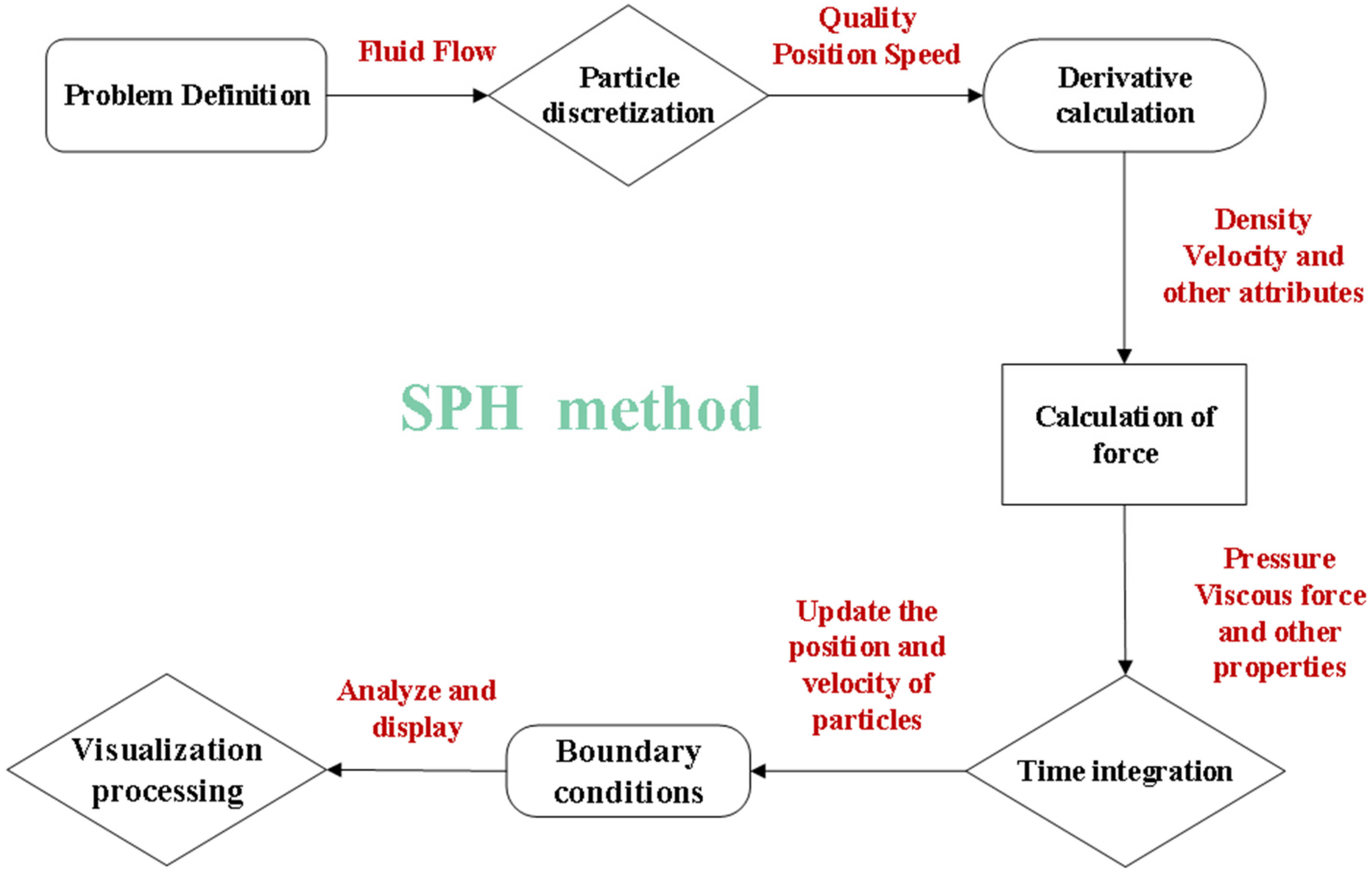
2. SPH Basic Theory
2.1. SPH Basic Ideas
2.2. SPH Basic Equation
2.3. SPH Method for Solving the N-S Equation
2.3.1. Navier–Stokes Equations
2.3.2. Density Particle Approximation Method for Solving the N-S Equation
2.4. Smooth Kernel Function Construction
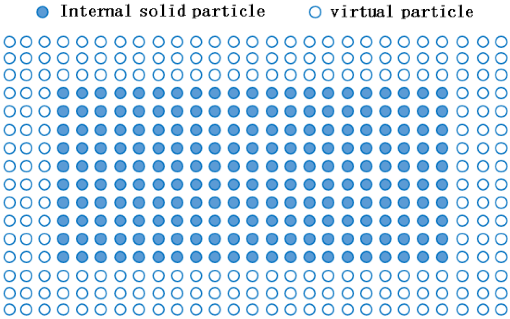
2.5. Other Key Technologies
3. Calculus Analysis
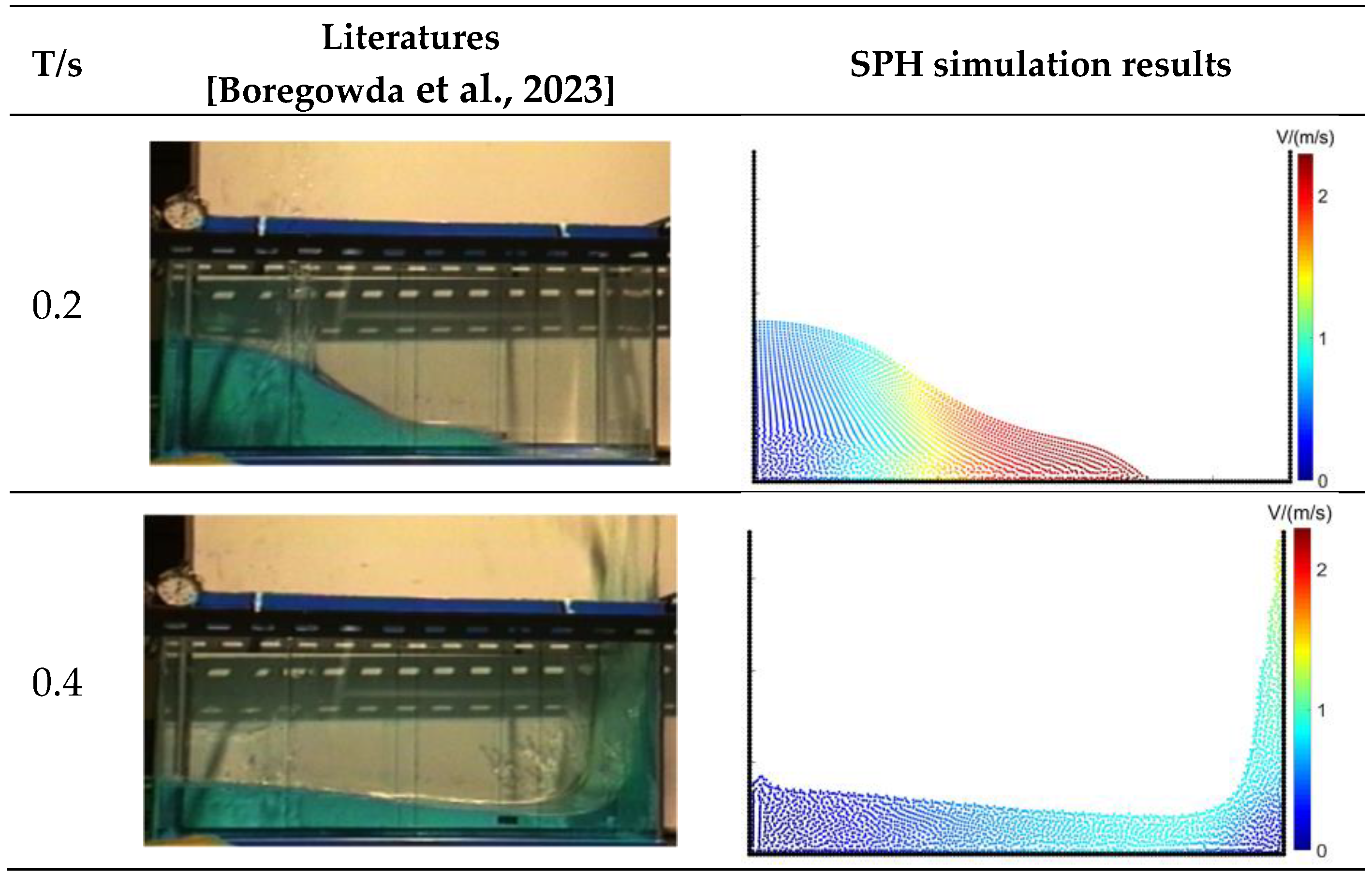
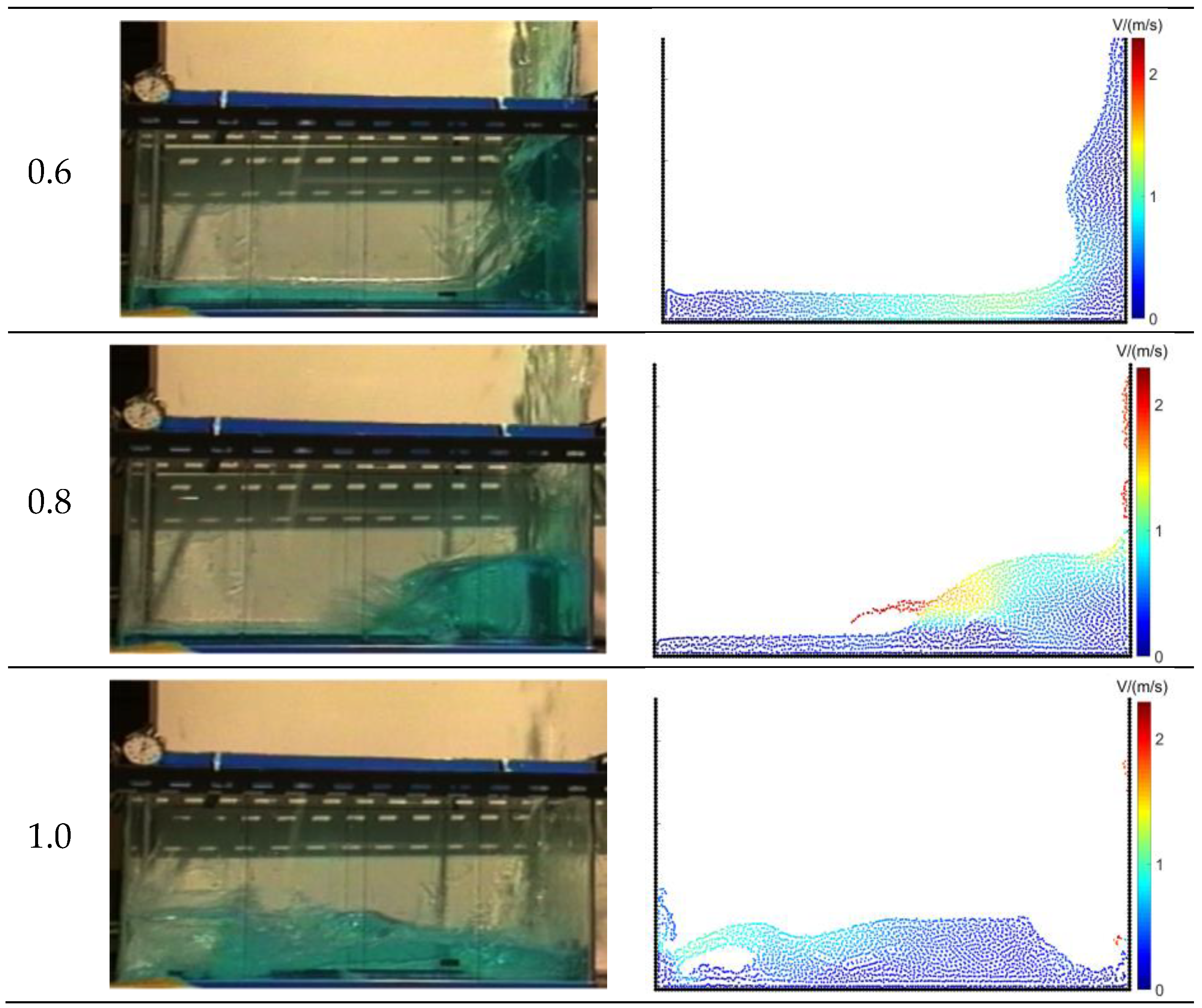
3.1. Transient Dam-Failure Arithmetic Simulation
3.2. Example Simulation of Gradual Collapse
- (1)
- The model has some improvements in the way the points are laid out, which can optimize the model to some extent for the traditional SPH dam-failure model;
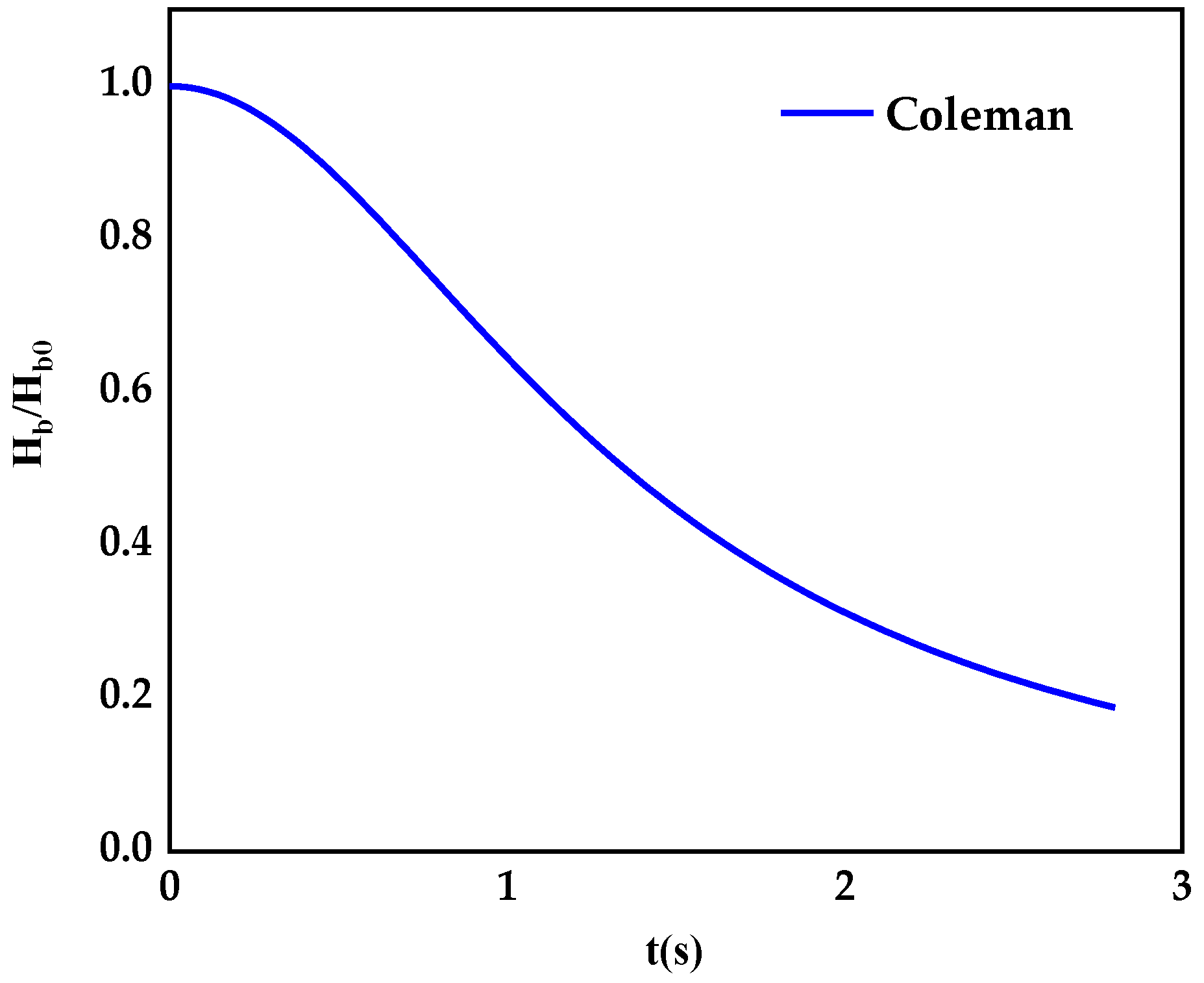
- (2)
- The model facilitates the development of later studies, and the calculation of the height of the initial dam height versus the height of the moment of failure over time can be analyzed in comparison with Coleman’s theoretical solutions in the literature.
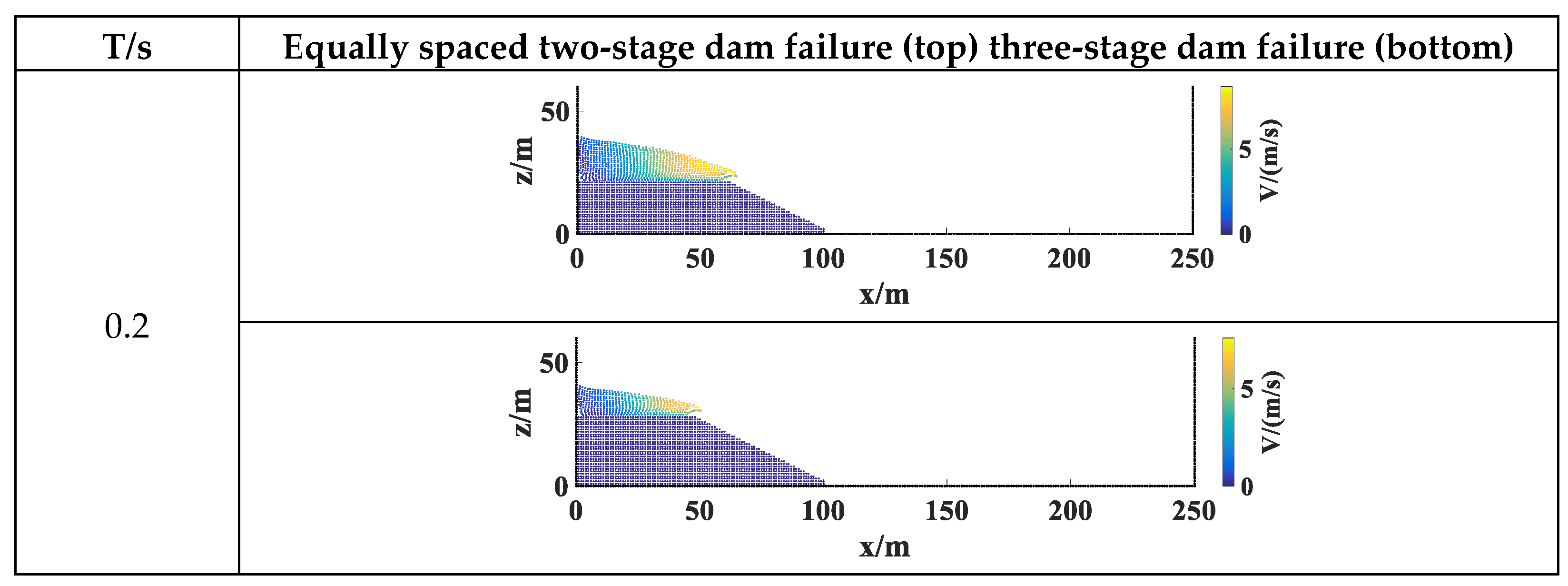
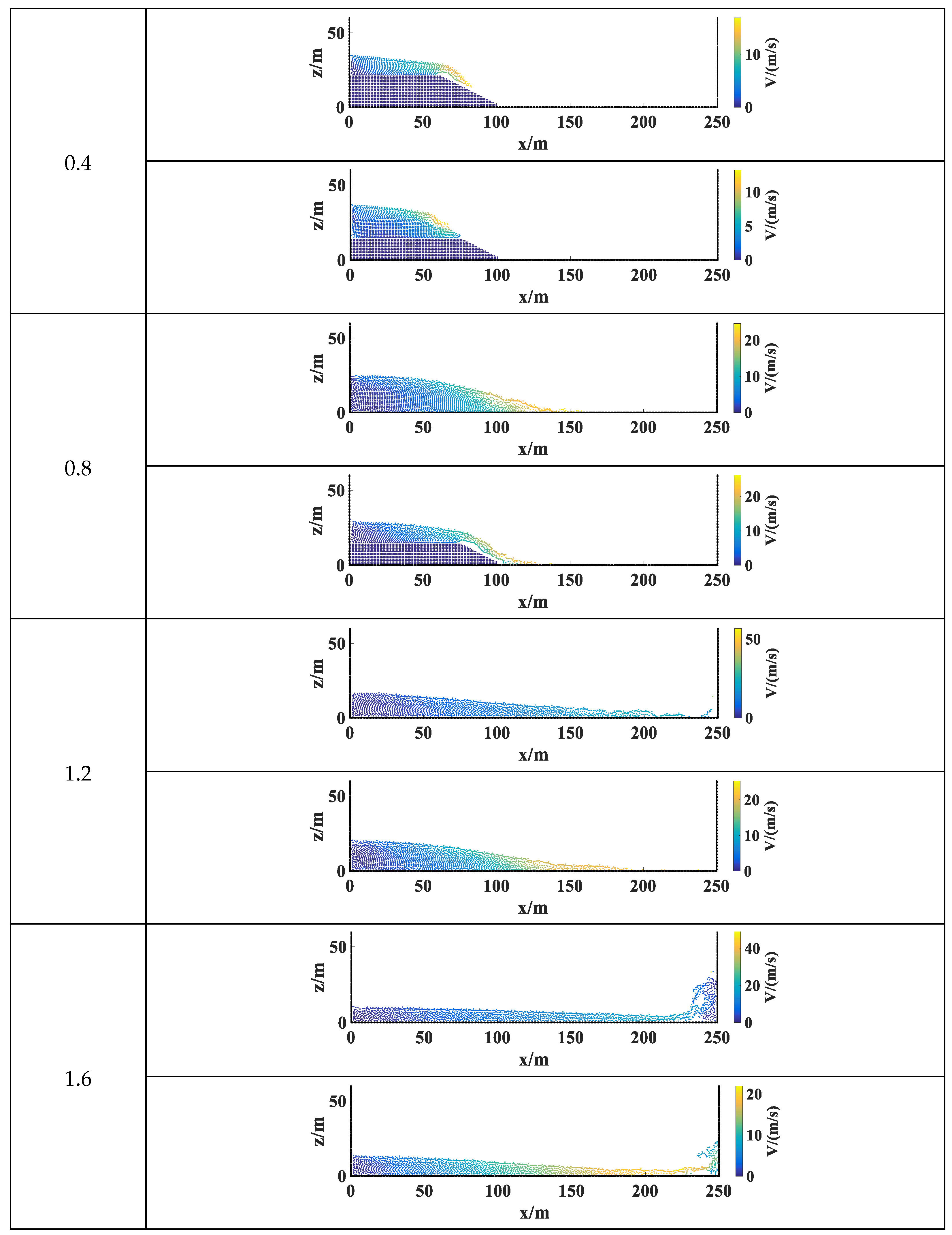
3.2.1. Equally Spaced Collapse Simulation
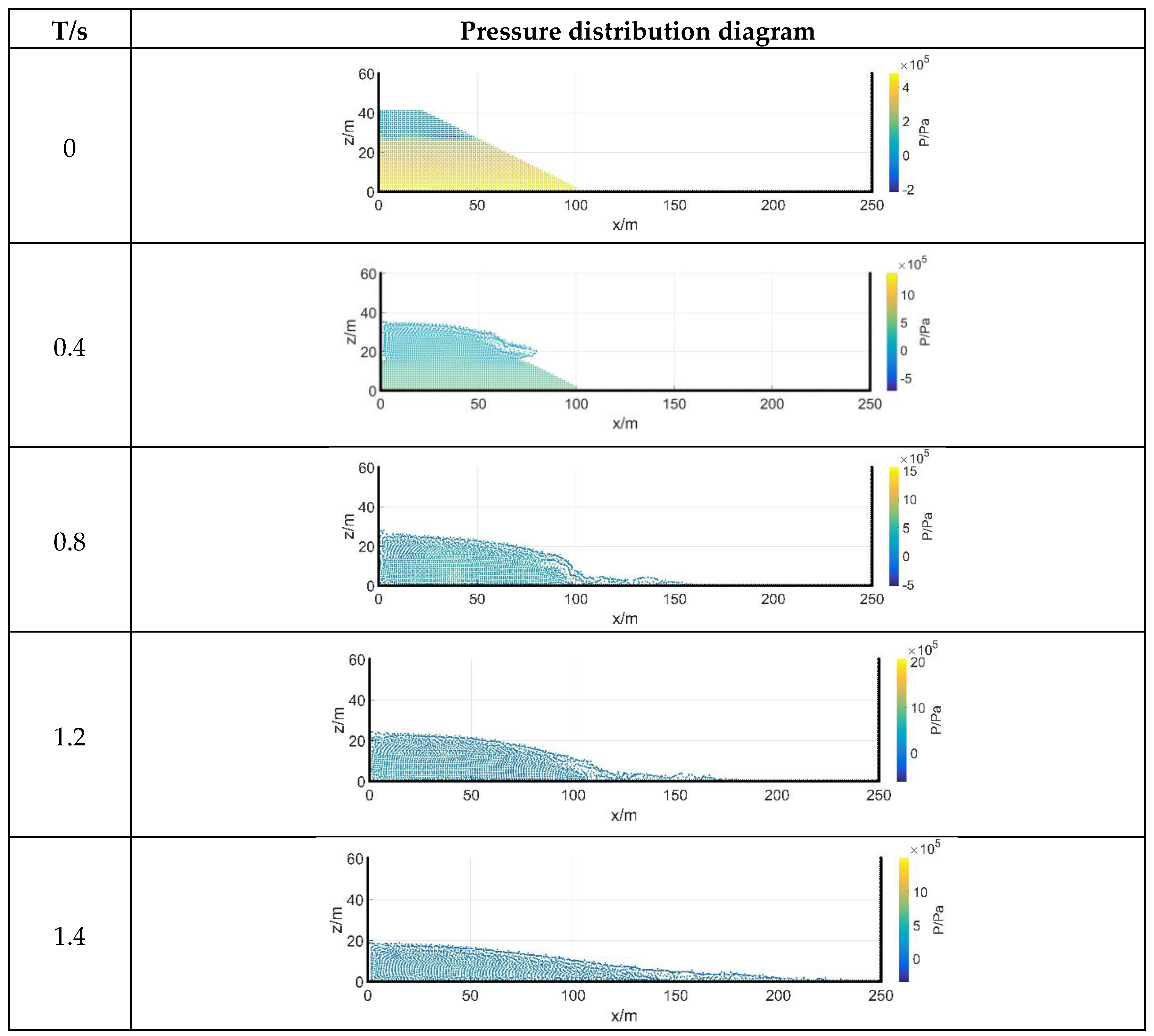
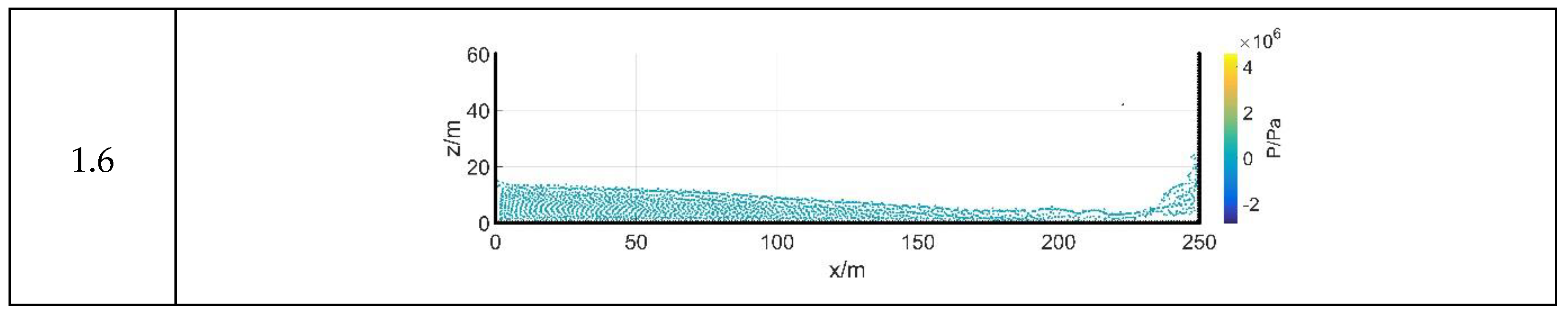
3.2.2. Progressive Collapse Simulation
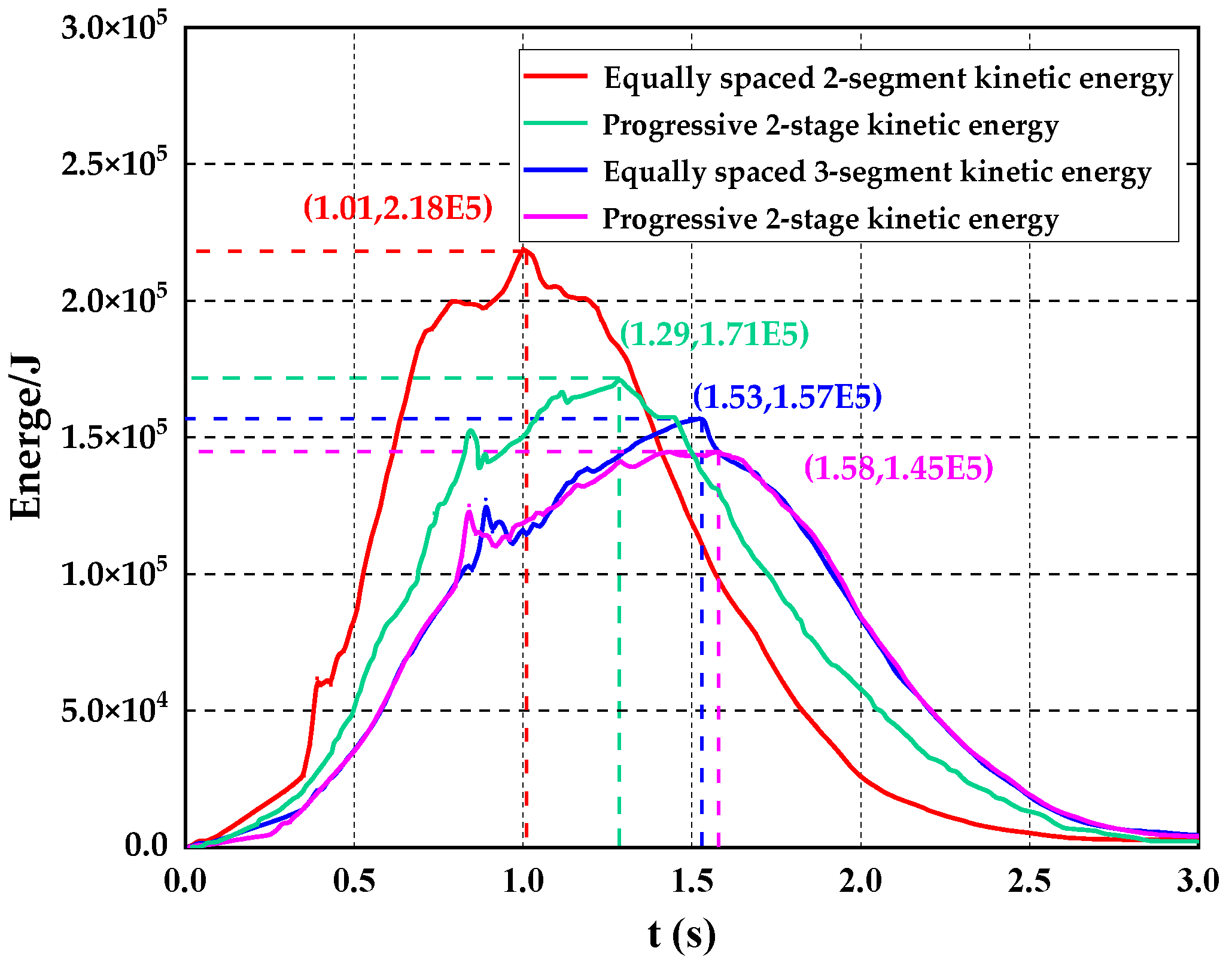
3.2.3. Analysis of Results
4. Conclusions
4.1. Conclusions
- The simulation of dam-failure flow using the smooth particle hydrodynamics (SPH) method, including the simulation of the classical dam-failure mode and the simulation of the step-by-step dam-failure mode, as well as the further division of the two modes of study of the equal-spaced and progressive modes were investigated to explore the failure modes in line with the dam-failure flow;
- Compared to instantaneous dam failure, the calculation results of the breach development considering the progressive gradual dam-failure model are more consistent with the theoretical solution and closer to the actual dam-failure process;
- Under multiple progressive dam-failure modes, as the number of segments increases, the degree of agreement between the calculated results of the breach development and the theoretical solution increases, and progressive dam failure has a higher degree of agreement than equal-interval dam failure, while the total kinetic energy of the breaching flood decreases with the increase in the number of segments of the progressive dam failure.
4.2. Outlook
Author Contributions
Funding
Data Availability Statement
Conflicts of Interest
References
- Ru, N. Dam Accidents and Safety; China Water Conservancy and Hydropower Press: Beijing, China, 1995. [Google Scholar]
- Jiang, J.; Yang, Z. Laws of dam failures of small-sized reservoirs and countermeasures. Chin. J. Geotech. Eng. 2008, 30, 1626–1631. [Google Scholar]
- Brufau, P.; Garcia-Navarro, P. Two-dimensional dam break flow simulation. Int. J. Numer. Methods Fluids 2000, 33, 35–37. [Google Scholar] [CrossRef]
- Shi, H.; Liu, Z. Research progress in numerical simulation of dam break flow. Adv. Water Sci. 2006, 17, 129–135. [Google Scholar]
- Hanson, G.; Cook, K.; Britton, S. Observed Erosion Processes During Embankment Overtopping Tests. In Proceedings of the 2003 ASAE Annual Meeting, Las Vegas, NV, USA, 27–30 July 2003. [Google Scholar]
- Alonso, E.E.; Gens, A. Aznalcóllar dam failure. Part 1: Field observations and material properties. Géotechnique 2006, 56, 165–183. [Google Scholar] [CrossRef]
- Zhang, H.; Hao, Z.; Feng, Z. Application of Lattice Boltzmann method to simulation of impact of droplet on liquid surface. J. Hydraul. Eng. 2008, 39, 1316–1320. [Google Scholar]
- Saikali, E.; Bilotta, G.; Hérault, A.; Zago, V. Accuracy Improvements for Single Precision Implementations of the SPH Method. Int. J. Comput. Fluid Dyn. 2020, 34, 774–787. [Google Scholar] [CrossRef]
- Wang, Z.; Li, D.; Li, Y.; Niu, J. Numerical studies on droplet impact to wettable solid boundary based on SPH method. Chin. Sci. Bull. 2017, 62, 2788–2795. [Google Scholar] [CrossRef]
- Chen, J.Y.; Feng, D.L.; Liu, J.H.; Yu, S.Y.; Lu, Y. Numerical Modeling of the Damage Mechanism of Concrete-soil Multilayered Medium Subjected to Underground Explosion Using the GPU-Accelerated SPH. Eng. Anal. Bound. Elem. 2023, 151, 265–274. [Google Scholar] [CrossRef]
- He, X.F.; Wang, Z.; Zhang, J.; He, Q. Simulation analysis of dam discharge process based on smooth particle hydrodynamics (SPH). SCIENTIA SINICA Technol. 2019, 49, 109–114. [Google Scholar] [CrossRef]
- Liu, J.; Bao, X.; Tan, H.; Wang, J.; Guo, D. Dynamical artificial boundary for fluid medium in wave motion problems. Chin. J. Theor. Appl. Mech. 2017, 49, 1418–1427. [Google Scholar]
- Du, T.; Wang, Y.; Huang, C.; Liao, L. Study on coupling effects of underwater launched vehicle. Chin. J. Theor. Appl. Mech. 2017, 49, 782–792. [Google Scholar]
- Chen, W.; Fu, Y.; Guo, S.; Jiang, C. Fluid-solid coupling and dynamic response of vortex-induced vibration of slender ocean cylinders. Adv. Mech. 2017, 47, 25–91. [Google Scholar]
- He, T.; Zhang, K.; Wang, T. AC-CBS-based partitioned semi-implicit coupling algorithm for fluid-structure interaction using sta-bilized second-order pressure scheme. Commun. Comput. Phys. 2017, 21, 1449–1474. [Google Scholar] [CrossRef]
- Liu, Z.-M.; Nan, S.; Shi, Y. Hemodynamic parameters analysis for coro-nary artery stenosis of intermediate severity model. Chin. J. Theor. Appl. Mech. 2017, 49, 1058–1064. [Google Scholar]
- Gingold, R.A.; Monaghan, J.J. Smoothed particle hydrodynamics: Theory and application to non-spherical stars. Mon. Not. R. Astron. Soc. 1977, 181, 375–389. [Google Scholar] [CrossRef]
- Colagrossi, A.; Landrini, M. Numerical simulation of interfacial flows by smoothed particle hydrodynamics. J. Comput. Phys. 2003, 191, 448–475. [Google Scholar] [CrossRef]
- Wang, Z.; Zhang, W. Impact of earthquake landslides on bridge piles based on parallel SPH method. J. Hunan Univ. 2022, 49, 54–65. [Google Scholar]
- Monaghan, J.J. Simulating Free Surface Flows with SPH. J. Comput. Phys. 1994, 110, 399–406. [Google Scholar] [CrossRef]
- Zhang, L.; Zhang, J. Comparative Study of SPH Method and LBM Method in Dam Break Flow Simulation Rural water conservancy and hydropower in China. China Rural. Water Hydropower 2020, 10, 234–241. [Google Scholar]
- Lo, E.; Shao, S. Simulation of Near-shore Solitary Wave Mechanics by an Incompressible SPH Method. Appl. Ocean. Res. 2002, 24, 275–286. [Google Scholar]
- Zhu, C.; Hu, N.; Zhang, X.; He, M.; Tao, Z.; Yin, Q.; Meng, Q. Numerical Simulation of Bidirectional Charge Accumulation Tensioning Blasting Based on Smooth Particle Flow Method. J. Cent. South Univ. (Nat. Sci. Ed.) 2022, 53, 2122–2133. [Google Scholar]
- Dalrymple, R.A.; Rogers, B.D. Numerical Modeling of Water Waves with the SPH Method. Coast. Eng. 2006, 53, 141–147. [Google Scholar] [CrossRef]
- Xu, X. An Improved SPH Method for Simulating 3D Dam Break Flows with Broken Waves. Comput. Methods Appl. Mech. Eng. 2016, 311, 723–742. [Google Scholar] [CrossRef]
- Boregowda, P.; Liu, G.-R. On the Accuracy of SPH Formula with Boundary Integral Terms. Math. Comput. Simul. 2023, 210, 320–345. [Google Scholar] [CrossRef]
- Gong, K.; Liu, Y.; Wang, B. Improvement of SPH fixed wall boundary treatment method. Chin. Q. Mech. 2008, 29, 507–514. [Google Scholar]
- Zhang, W.; Gao, Y.; Huang, Y.; Maeda, K. Normalized correction of soil-water-coupled SPH model and its application. J. Geotech. Eng. 2018, 40, 262–269. [Google Scholar]
- Wang, Z.; Li, D.; Hu, Y. A SPH stress correction algorithm and its application in free surface flow. Chin. J. Comput. Mech. 2017, 34, 101–105. [Google Scholar]
- Wu, K.; Yang, D.; Wright, N. A Coupled SPH-DEM Model for Fluid-Structure Interaction Problems with Free-surface Flow and Structural Failure. Comput. Struct. 2016, 177, 141–161. [Google Scholar] [CrossRef]
- Coleman, S.E.; Andrews, D.P.; Webby, M.G. Overturning failure of non cohesive homogeneous embankment. J. Hydraul. Eng. 2002, 128, 829–838. [Google Scholar] [CrossRef]
- Liu, J.; Li, L.; Lin, Y.; Chen, W.; Li, X. Depth Erosion and Tracing of Overtopping Landslide Dam Breach. J. Jilin Univ. 2020, 50, 183–191. [Google Scholar]


| Serial Number | Calculation Condition | Parameter Condition |
|---|---|---|
| 1 | Total number of particles | 2812 |
| 2 | Boundary particle spacing | 0.0026 |
| 3 | SPH particle spacing | 0.0038 |
| 4 | Fluid density/(kg/m3) | 1000 |
| 5 | Kernel function type | Cubic spline function |
| 6 | Density approximation methods | Approximation of the continuity equation |
| 7 | Time step | 0.0001 s |
| 8 | Smooth length | 1.25 particle spacing |
| 9 | Coefficient of viscosity | 1.2 |
| 10 | Time | 1.0 |
| Time | T = 0.2 s | T = 0.4 s | T = 0.8 s | Average |
|---|---|---|---|---|
| Similarity | 92.1% | 90.7% | 82.3% | 88.4% |
| Serial Number | Calculation Condition | Parameter Condition |
|---|---|---|
| 1 | Total number of particles | 2911 |
| 2 | Boundary particle spacing/m | 1 |
| 3 | SPH particle spacing/m | 1 |
| 4 | Kernel function type | Cubic spline function |
| 5 | Density approximation methods | Approximation of the continuity equation |
| 6 | Time step | 0.0001 s |
| 7 | Smooth length h | 1.25 particle spacing |
| 8 | Fluid density/(kg/m3) | 1000 |
| 9 | Coefficient of viscosity | 1.2 |
| 10 | Time/s | 2.0 |
| Gradual Dam-Failure Condition | 2 Paragraph | 3 Paragraph | 4 Paragraph | 5 Paragraph |
|---|---|---|---|---|
| Equidistant dam failure | 72.2% | 85.9% | 92% | 95.4% |
| Progressive dam failure | 79.1% | 95.2% | 96.9% | 97.1% |
Disclaimer/Publisher’s Note: The statements, opinions and data contained in all publications are solely those of the individual author(s) and contributor(s) and not of MDPI and/or the editor(s). MDPI and/or the editor(s) disclaim responsibility for any injury to people or property resulting from any ideas, methods, instructions or products referred to in the content. |
© 2023 by the authors. Licensee MDPI, Basel, Switzerland. This article is an open access article distributed under the terms and conditions of the Creative Commons Attribution (CC BY) license (https://creativecommons.org/licenses/by/4.0/).
Share and Cite
Zhang, J.; Wang, B.; Li, H.; Zhang, F.; Wu, W.; Hu, Z.; Deng, C. Progressive Dam-Failure Assessment by Smooth Particle Hydrodynamics (SPH) Method. Water 2023, 15, 3869. https://doi.org/10.3390/w15213869
Zhang J, Wang B, Li H, Zhang F, Wu W, Hu Z, Deng C. Progressive Dam-Failure Assessment by Smooth Particle Hydrodynamics (SPH) Method. Water. 2023; 15(21):3869. https://doi.org/10.3390/w15213869
Chicago/Turabian StyleZhang, Jianwei, Bingpeng Wang, Huokun Li, Fuhong Zhang, Weitao Wu, Zixu Hu, and Chengchi Deng. 2023. "Progressive Dam-Failure Assessment by Smooth Particle Hydrodynamics (SPH) Method" Water 15, no. 21: 3869. https://doi.org/10.3390/w15213869
APA StyleZhang, J., Wang, B., Li, H., Zhang, F., Wu, W., Hu, Z., & Deng, C. (2023). Progressive Dam-Failure Assessment by Smooth Particle Hydrodynamics (SPH) Method. Water, 15(21), 3869. https://doi.org/10.3390/w15213869