Abstract
Canopy resistance is a key parameter in the Penman–Monteith (P–M) equation for calculating evapotranspiration (ET). In this study, we compared a machine learning algorithm–support vector machine (SVM) and an analytical solution (Todorovic, 1999) for estimating canopy resistances. Then, these estimated canopy resistances were applied to the P–M equation for estimating ET; as a benchmark, a constant (fixed) canopy resistance was also adopted for ET estimations. ET data were measured using the eddy-covariance method above three sites: a grassland (south Ireland), Cypress forest (north Taiwan), and Cryptomeria forest (central Taiwan) were used to test the accuracy of the above two methods. The observed canopy resistance was derived from rearranging the P–M equation. From the measurements, the average canopy resistances for the grassland, Cypress forest, and Cryptomeria forest were 163, 346, and 321 (s/m), respectively. Our results show that both methods tend to reproduce canopy resistances within a certain range of intervals. In general, the SVM model performs better, and the analytical solution systematically underestimates the canopy resistances and leads to an overestimation of evapotranspiration. It is found that the analytical solution is only suitable for low canopy resistance (less than 100 s/m) conditions.
1. Introduction
Evapotranspiration (or latent heat flux, LE) is a crucial subject in understanding water cycles, micrometeorology, and climate change. Information about LE can be applied to research focusing on cooling effects, energy balances in green roofs, and water resource management for reservoirs and agriculture. Furthermore, it constitutes fundamental knowledge for achieving the United Nations Sustainable Development Goals, particularly in the realms of sustainable cities and communities (Goal #11) and climate action (Goal #13).
Among the various methods for estimating evapotranspiration, the Penman–Monteith (P–M) equation is the most widely adopted one [1]. For instance, the Food and Agriculture Organization (FAO) of the United Nations utilizes the P–M equation to estimate crop evapotranspiration. This method primarily combines the Monin–Obukhov similarity theory (MOST) with the resistance concept and utilizes measured net radiation, soil heat flux, air temperature, humidity, and wind speed to estimate evapotranspiration. However, this method also requires two additional parameters: aerodynamic resistance (ra) and surface resistance (rs). When the surface is covered by water, rs is equal to zero. When the surface is densely covered with vegetation, rs represents the canopy resistance (rc). The aerodynamic resistance can be calculated using the MOST. The major challenge with the P–M equation is the requirement for accurate surface (or canopy) resistances [2,3,4].
Canopy resistances can be obtained from historical observed values or calculated using analytical or statistical models. The FAO [1] adopted a constant value of rc (=70 s/m) in the P–M equation to estimate the reference evapotranspiration. This reference evapotranspiration is further multiplied by a crop coefficient to calculate the actual evapotranspiration. While this method is straightforward, it is considered less accurate [5,6]. In addition to using a fixed (constant) canopy resistance in the P–M equation, using variable canopy resistance estimated from models is also adopted.
Many parameterization models [7,8,9,10,11] expressed rc as a function of meteorological variables (such as net radiation, wind speed, relative humidity, and air temperature). The Jarvis multiplicative model [7] stands as a representative example of such models. However, calibrations of regression coefficients for different vegetation types and meteorological conditions are required before using such models. Founded upon certain assumptions, Todorovic [12] proposed a mechanistic approach (analytical solution) to calculate canopy resistance; his model is also a function of climatic variables and aerodynamic resistance, but no calibration coefficients are needed. Pauwels and Samson [13] found that rc calculated from Todorovic’s equation has some problems above a wet, sloping grassland. On the other hand, Lecina et al. [14] and Perez et al. [15] recommended Todorovic’s model for semiarid conditions. Perez et al. [15] also found that through a constant canopy resistance, there could be an underestimate of evapotranspiration in the summer and an overestimate in the winter; it was shown that using a monthly averaged surface resistance instead of a constant value would lead to a better estimation of evapotranspiration at seasonal time scale. Li et al. [16] studied surface resistances under arid conditions with a dense canopy (maize field) and a partial canopy (vineyard). Their results showed that Todorovic’s method performed poorly in both cases, while the Jarvis multiplicative model performed better on dense canopy than partial canopy.
In addition to estimating LE by the P–M equation in conjunction with rc estimated from Todorovic’s or parameterization methods, machine learning (ML) models have also gained widespread use for the estimations of surface fluxes in recent times [17,18]. However, as far as our current knowledge goes, there are no published studies using ML approaches to estimate canopy resistance. Huang and Hsieh [19] employed five ML models, including support vector machine (SVM), random forest, multi-layer perceptron, deep neural network, and long short-term memory, for the gap-filling of surface fluxes. They concluded that the five ML models performed well and similarly for estimating sensible heat, latent heat, and CO2 fluxes, and SVM is a little bit better than the other four ML models in LE estimations.
According to previous studies, canopy resistance estimation methods have different specific responses to different climatic conditions and vegetation surfaces. Therefore, the objectives of this study are (1) to study the SVM model and Todorovic’s analytical equation for estimating canopy resistance over three different ecosystems: a humid grassland, a mountain Cypress forest, and a mountain Cryptomeria forest; (2) to integrate these two model estimated canopy resistances with the P–M equation to estimate evapotranspiration, and compare with measured values to assess the performance of each model. To the best of our knowledge, previous studies have mainly focused on using physical process models or machine learning approaches for flux estimations. This study is the first to employ a ML model for estimating canopy resistance and integrate it with a physical process model (P–M equation) for predicting evapotranspiration.
2. Sites and Data
The study sites include a grassland, a Cypress forest, and a Cryptomeria forest. Detailed descriptions for these three areas and experiments are provided in Section 2.1, Section 2.2 and Section 2.3 and summarized in Table 1. Section 2.4 introduces the procedure of data processing.

Table 1.
Summary of site features and instrumental heights.
2.1. Dripsey Grassland Experiment
The grassland experimental site is located in Dripsey, County Cork, southwestern Ireland (latitude 51°59′ N; longitude 8°46′ W), with an average elevation of 200 m. The climate in this area is mild and humid, with an annual average temperature of 9.6 °C and an annual average precipitation of 1222.7 mm. The data of this study area cover the period from 1 January 2013 to 31 December 2013.
The dominant plant species in the area is perennial ryegrass (Lolium perenne L.), with vegetation heights ranging from 0.2 to 0.45 m during the summer. The leaf area index for summer and winter is approximately 2.0–2.5 m2/m2 and 0.5–1.0 m2/m2, respectively.
The experiment employed a tipping bucket rain gauge (ARG100, Environmental Measurements Ltd., North Shields, UK) to measure precipitation. Net radiation was measured using a net radiometer (CNR1, Kipp & Zonen, Lincoln, UK). Air temperature and humidity were recorded using a temperature and humidity sensor (HMP45C, Campbell Scientific, North Logan, UT, USA). These instruments were installed at heights of 0, 4, and 2.5 m above the ground, respectively. Soil heat flux at 0.1 m below the ground was measured using a heat flux plate (HFP01, Hukseflux, Delft, The Netherlands); soil temperature sensors were also installed at 1.5, 5, and 7.5 cm to measure the soil temperature and to calculate the heat storage in this soil layer. The soil heat flux at the ground surface was then calculated as the sum of the soil heat flux at 0.1 m depth and the heat storage in this layer. All meteorological measurements were taken at a 1 min sampling frequency, and all data were averaged every 30 min. The CR23X data logger (Campbell Scientific) was employed to record all averaged data.
In this study, surface fluxes were measured using the eddy-covariance method. Three-dimensional wind speeds were measured using a 3-D sonic anemometer (CSAT3, Campbell Scientific), while water vapor and carbon dioxide concentrations were measured using an open-path infrared gas analyzer (LI-7500, Li-Cor). Both of these instruments were installed at 5 m above the ground. All data were recorded at a frequency of 10 Hz and averaged every 30 min. Further details regarding the experimental data can be found in Peichl et al. [20].
2.2. Chi-Lan Forest Experiment
This Chi-Lan forest site is a uniform Cypress montane forest in northeastern Taiwan (24°35′ N, 121°30′ E). Meteorological data and surface flux measurements were conducted at a walk-up tower (elevation of 1650 m) from 1 May 2005 to 30 April 2007. The location is frequently covered by fog and clouds, resulting in relatively reduced solar radiation. According to historical records, the annual average temperature is around 13 °C, and the annual precipitation is approximately 4000 mm. Due to the frequent precipitation, the soil moisture at 30 cm depth is approximately 0.3–0.4 m3/m3, and this value remains relatively stable. The soil moisture conditions have a minimal impact on daily evapotranspiration and do not play a dominant role in the water resource cycle in this Cypress forest. The canopy in this study site was closed and uniform, with an average canopy height of 10.3 m and a leaf area index of 6.3 m2/m2. As a result, the soil heat flux at the surface was quite low, ranging from −15 to 25 W m−2 throughout the year. The soil heat flux at 0.1 m and soil temperature at 0.05 m below the ground were measured using a heat flux plate (HFP01) and a soil temperature sensor.
In this experiment, in addition to the primary meteorological data, we also employed the eddy-covariance method to measure the surface fluxes in this study area. The meteorological instruments were installed on a 23.4 m tall meteorological tower situated in an area with flat terrain. The net radiation was measured using a CNR1 radiometer (Kipp & Zonen), which measured both upward and downward shortwave and longwave radiation components. The radiometer was installed at 22.5 m. Air temperature and humidity were measured using an HMP45A (Vaisala, Vantaa, Finland) sensor positioned at 23.6 m. The measured data were transmitted to a data logger (CR23X) and averaged every 30 min. The eddy-covariance system was installed at 24 m above the ground and consisted of an R.M. Young 81000 ultrasonic anemometer for measuring 3-D wind speed and air temperature and an open-path infrared gas analyzer (LI-7500, Li-Cor) for measuring water vapor and CO2 concentrations. The sampling frequency of the eddy-covariance system was 10 Hz, and the data were averaged and recorded every 30 min. More detailed information can be found in Chu et al. [21]
2.3. Sitou Forest Experiment
The Sitou forest site is located in Nantou County, central Taiwan. This site is part of the Experimental Forest of National Taiwan University. Due to its location in a subtropical monsoon climate zone, the climate is warm and humid. Additionally, the area frequently experiences fog and mist during the autumn and winter seasons. Based on its historical data, the annual average temperature is 16.6 °C, the average humidity is 89%, and the annual rainfall is 2635 mm. The experimental forest covers an area of approximately 2500 hectares and spans an elevation range from 800 to 2000 m. Within this forested area, there are two meteorological towers (Tower A and B) situated in the Japanese cedar (Cryptomeria) region. These towers are located at an elevation of approximately 1250 m. The area of this Cryptomeria region is about 80 hectares and has an average slope of 13.6°. The average canopy height was about 26 m. Tower A (23°39′50′′ N, 120°47′46′′ E) is located at an elevation of 1252 m. Tower B (23°39′51′′ N, 120°47′45′′ E) is situated approximately 64 m away from Tower A. The heights of Tower A and B are 35 and 40 m, respectively. The measurements used in these data were collected from Tower A.
In this site, surface fluxes were also measured using the eddy-covariance method. The open-path eddy-covariance system was installed on Tower A at a height of 28 m above the ground. This system included a 3-D sonic anemometer (CSAT3, Campbell Scientific) for measuring wind speeds and an open-path gas analyzer (Li-7500, Li-Cor) for measuring CO2 and H2O concentrations. Additionally, a data logger was used to collect data at 10 Hz, with the averages taken every 30 min. For meteorological data, a net radiometer (NR-LITE) and a rain gauge (TE525MM) were installed to measure net radiation and precipitation. At 27.5 m above the ground, temperature and humidity measurements were collected using a temperature and humidity sensor (HMP45C); at the same height, a precision infrared temperature sensor (IRTS-P) was used to measure canopy surface temperature. Soil heat flux at 0.05 m below the ground was measured using a heat flux plate (HFP01); a soil temperature sensor was also installed at 5 cm depth to measure the soil temperature for calculating the heat storage in this soil layer. All meteorological data were connected to a data logger (CR23X) with a sampling frequency of 30 s and an averaging period of 30 min. The data collection period for this study was from 22 May 2009 to 31 July 2010.
2.4. Data Processing
For calculating surface fluxes from the eddy-covariance system, the general standard data processing procedure [22] was completed, which included (1) a double rotation of the x coordinate to be along with the mean wind direction; (2) the Webb, Pearman, and Leuning correction [23]. For the purpose of this study, the following data selection criteria were applied.
- (1)
- In the evening, due to small evapotranspiration, the measured canopy resistance calculated from Equation (3) can be unreasonably large; hence, only daytime data (Rn > 0) were used for this study.
- (2)
- If a measured rc is less than 0 or larger than 1050 s/m, this data point is not reliable and excluded from further analysis.
- (3)
- Obvious outliers and anomalies values in the data were removed.
Based on the findings of Huang and Hsieh [19], considering the time factor can effectively enhance the accuracy of surface flux gap-filling for certain ecosystems. Therefore, in this study, the input factors for ML predictions of rc are (1) time factor (i.e., Julian day) and (2) meteorological factors (i.e., available energy, air temperature, wind speed, and vapor pressure deficit). These input factors for training the ML model are also summarized in Table 2. To build the ML model, the ratio of training and testing datasets is 6:4. Each dataset is sorted chronologically, with the first 60% used for training and the remaining 40% used for validation.
Table 2.
List of input factors used in the support vector machine model.
3. Methods
3.1. Penman–Monteith Equation
The P–M equation for estimating the actual evapotranspiration from a vegetated surface can be expressed as [24,25]
where LE is the latent heat flux (W/m2), Δ (kPa K−1) is the slope of the saturation vapor pressure-temperature curve calculated at the air temperature Ta, γ (=ρCp/0.622Lv) (kPa K−1) denotes psychrometric constant, ρ is the air density, Cp (=1005 J kg−1 K−1) is the specific heat of air, Lv (=2.46 × 10⁶ J kg−1) represents the latent heat of vaporization, Qn (=Rn–G) is the available energy, where Rn (W m−2) and G (W m−2) stand for the net radiation and soil heat flux at the ground surface, respectively, D (kPa) represents vapor pressure deficit, ra (s m−1) is the aerodynamic resistance, and rc (s m−1) is the canopy resistance. Note that for a vegetated surface and the canopy is closed, the surface resistance equals the canopy resistance, and the soil evaporation can be ignored. The term ra in Equation (1) can be calculated using MOST [26]:
where U (m/s) represents the wind speed, z (m) is the measurement height, d (m) stands for the zero-plane displacement (≈2/3 h), h (m) is the canopy height, z0m (m) is the roughness length for momentum (≈0.1 h), z0v (m) is the roughness length for water vapor (≈0.01 h), k (=0.4) is the von Kármán constant.
By rearranging Equation (1), the measured rc is computed as
with measured Qn and LE.
3.2. Todorovic’s Analytical Equation
Todorovic [11] assumed that if the vegetated surface is not fully wet (rc > 0), part of the available energy is required to heat the canopy to extract water. Therefore, this additional energy (H’) would raise the canopy temperature by an amount t, which is the temperature difference between the mean level (d + z0m) of source or sink for H and LE and the level in canopy (i.e., saturated level). Todorovic [11] then expressed LE as the difference between the potential evapotranspiration (PET) and H’, which is
where H’ is expressed as
In Equation (5), r′ is the “pseudo” resistance for heat transferred from the evaporating plant surface to d + z0m. A linear relationship between saturation vapor pressure and temperature and neutral atmospheric conditions were assumed by Todorovic [11]. As a result, the temperature difference, t, in Equation (5) could be calculated as
Todorovic argued that r′ is close to rc and then rc could be solved analytically by a quadratic equation as
By Equation (7), the solution for rc is
where
In Equations (7)–(11), ri is the isothermal resistance first introduced by Monteith [24] and defined as
The isothermal resistance (ri) is simply the sum of rc + ra under the isothermal condition , in which H = 0 and LE = Rn−G.
The beauty of Todorovic’s approach is that only meteorological variables are needed for solving rc and no training data are needed a priori.
Now, by substituting Equations (1), (5) and (6) into (4), we have
If for a site where the vapor pressure deficit is close to zero, Equation (13) becomes
Equation (14) is true only if rc = 0; in other words, Todorovic’s analytical solution is valid for the sites where rc is small. Equation (14) provides the limitation where this analytical solution for rc can be applied.
3.3. Constant Canopy Resistance Method
For a comparative baseline (benchmark), a fixed (constant) rc in the P–M equation for estimating LE was also used in this study. The determination of the constant rc followed an average calculation approach. That is, the preprocessed data underwent Equation (3) to calculate the measured canopy resistance for each time step. Subsequently, the average of all calculated canopy resistances was taken as the constant rc.
3.4. Support Vector Machine
The SVM is a ML algorithm introduced by Vladimir Vapnik in 1990. Initially, it was developed for classification tasks involving large datasets. Until 1995, Vapnik improved the algorithm to be used for regression problems. The application of SVM to regression problems is also referred to as support vector regression. In this study, we use the term SVM to encompass both classification and regression applications.
The SVM method offers two main advantages:
- (1)
- Balancing model accuracy and complexity: SVM utilized the principle of structural risk minimization to estimate the classification or regression hyperplane. By finding a decision boundary that maximizes the separation between classes or regression targets, SVM effectively delineates data points of different categories within a high-dimensional plane. This approach sets SVM apart from other ML methods as it simultaneously balances accuracy and model complexity. While enhancing model accuracy, it also helps mitigate issues like overfitting and excessive computational time.
- (2)
- Simplified weight estimation process: The process of weight determination in SVM is simplified into a quadratic programming problem, making it solvable using a standardization procedure.
In this study, the SVM was implemented using the Scikit-Learn package (version 0.22.1) in Python (version 3.6). The hyperparameters of the SVM model were tuned using a grid-search method. The candidate hyperparameters for SVM include kernel function (radial basis function and linear function), penalty coefficient, and the Gamma value used in the radial basis function kernel. The search range for the penalty coefficient and Gamma value was set between 2–5 and 25. For a more comprehensive understanding of SVM, the details can be found in Cork and Vapnik [27].
4. Results and Discussion
4.1. Diurnal Variations in Observed rc and LE
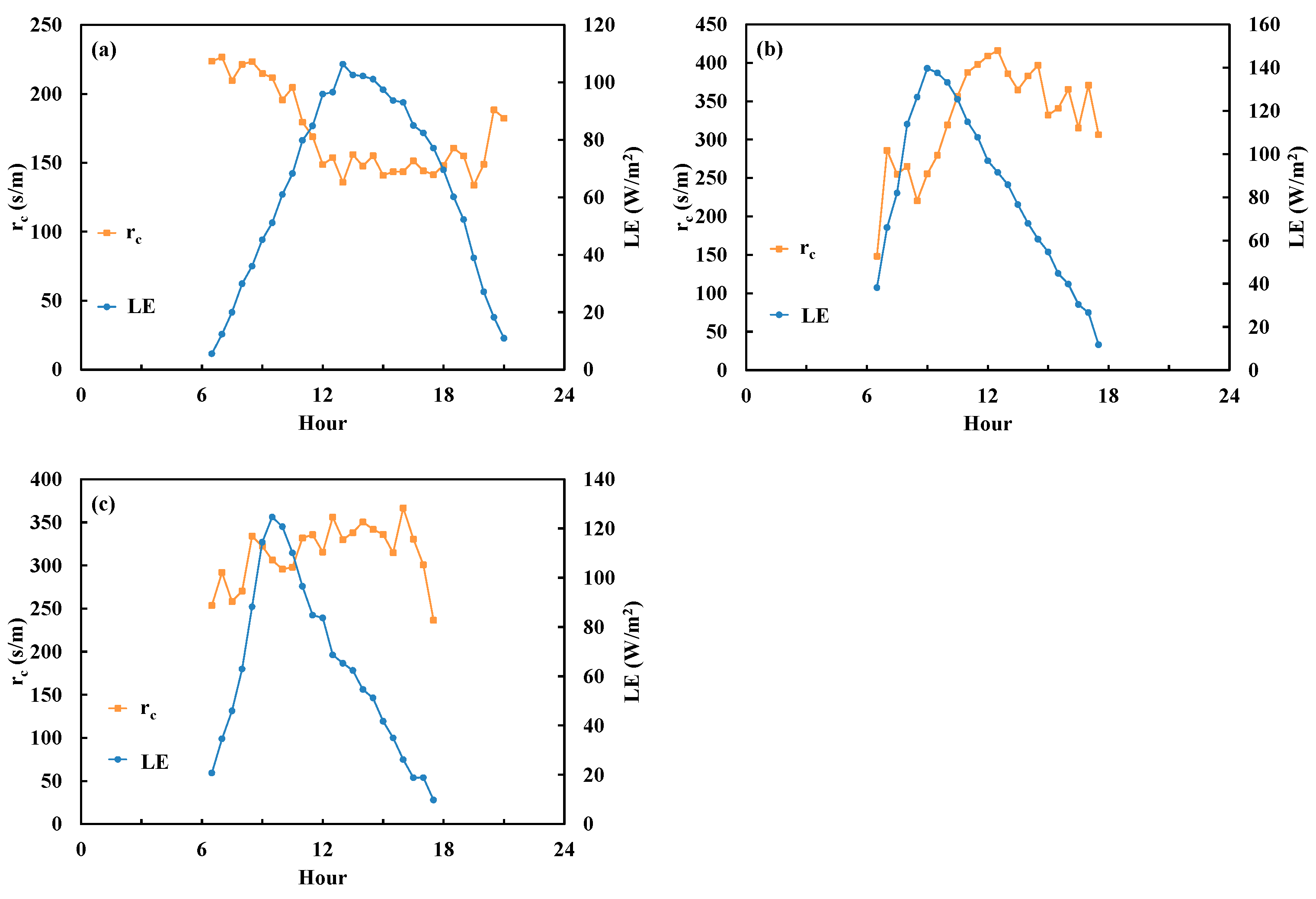
To examine the mean diurnal variations in rc and LE during the daytime (Grassland site: 06:30–21:00; forest sites: 06:30–17:30), we plotted the mean (averaged over the entire observation period) rc and LE as a function of local time (Figure 1). Notice that for the grassland, rc was larger in the early morning and then decreased to its lowest value (around 150 s/m) at 12:00 and maintained this value till 18:00 (Figure 1a).
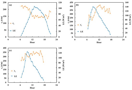
Figure 1.
Diurnal variations in canopy resistance (rc) and latent heat flux (LE) above (a) Dripsey grassland, (b) Chi-Lan forest, and (c) Sitou forest.
In contrast to the grassland area, both the Chi-Lan and Sitou forests exhibit a distinct pattern (Figure 1b,c). In these areas, rc was the lowest during the sunrise period (around 06:30) and then increased to its largest value around noon (12:00). This phenomenon is attributed to the presence of abundant dew on forest vegetation and the prevalence of fog, creating an environment akin to a wet surface in the early morning. As a result, the rc was lower, then subsequent to the evaporation of dew and the dispersal of fog, the rc gradually increased as the canopy became drier.
As to the diurnal variation in LE, Figure 1a shows that the peak LE happened around 12:00 at the grassland, but the maximum LE happened earlier (around 9:00) for both the forest sites (Figure 1b,c). This early LE peak for this kind of cloud-foggy forest can be attributed to the water that remained on the leaf surface from the early morning (see Gu et al. [28]).
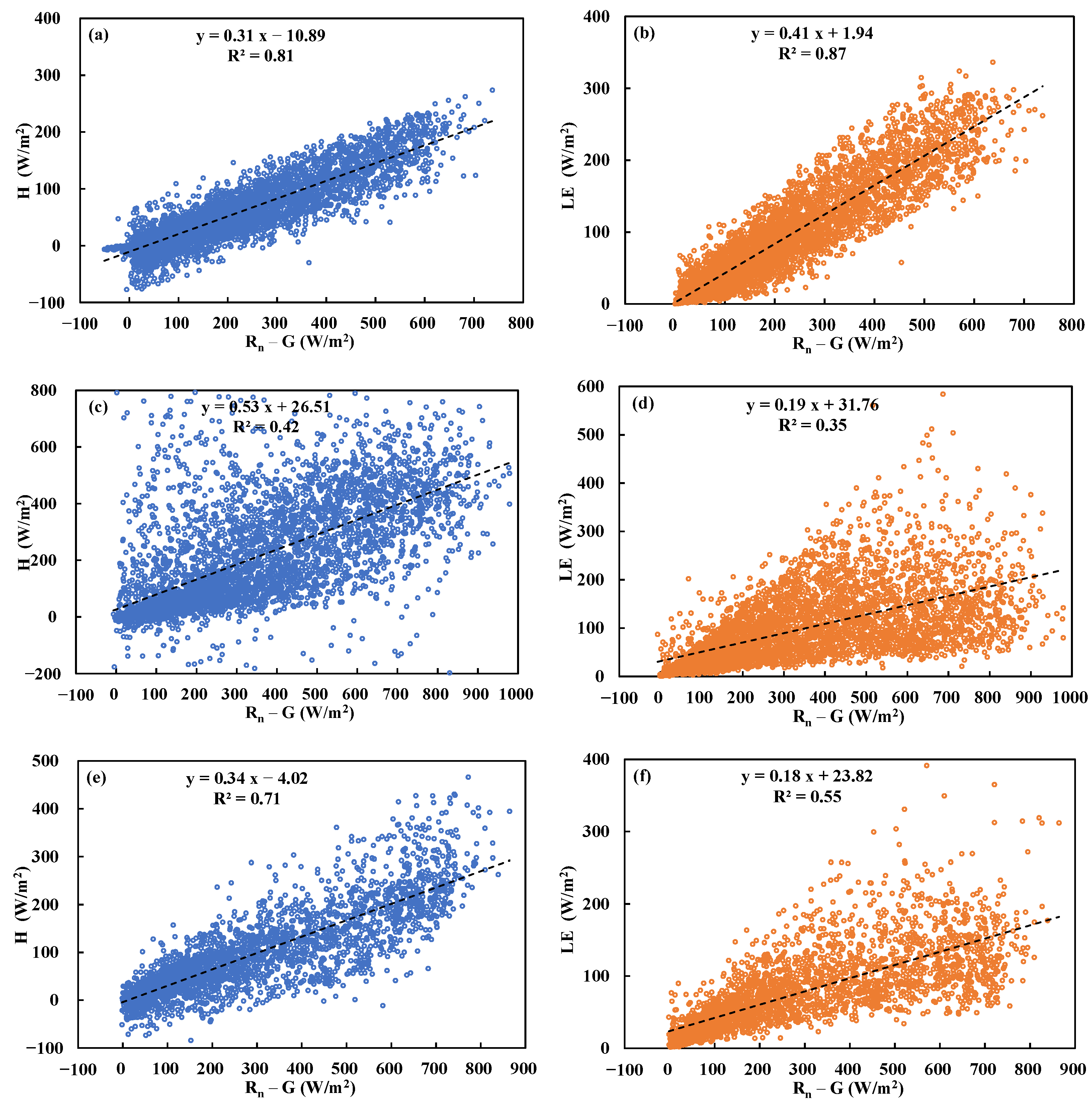
To check the energy closure rate and energy partition ratio, Figure 2 shows the scatter plots of sensible heat (H) and latent heat (LE) as a function of available energy (Rn–G). From Figure 2a,b, it can be inferred that in the Dripsey grassland, approximately 31% of the available energy is allocated to sensible heat flux, while about 41% is distributed to LE. The overall energy closure rate is 72%. On the other hand, for the Chi-Lan forest, the available energy is distributed with approximately 53% and 19% to sensible heat and latent heat fluxes, respectively. As for Sitou forest, the distribution of available energy is approximately 34% to H and 18% to LE. In the grassland, the available energy contributed in similar proportions to heating air and evapotranspiration. However, in the forests, a majority of the energy was utilized for sensible heat flux, with only a small portion being allocated to evapotranspiration. The energy closure ratios for Dripsey grassland and Chi-Lan forest are around 72% and are normal compared with the literature. The discrepancy in energy closure rate (only 52%) in the Sitou forest might predominantly arise from the storage of some Rn energy within the canopy layer. The lack of energy closure indicates that in these study areas, when using the P–M equation with available energy (Rn–G) for predicting LE, there might be an overestimation of LE.

Figure 2.
Scatter plots of sensible heat (H) and latent heat (LE) fluxes as a function of Rn−G above the Dripsey grassland (a,b), Chi-Lan forest (c,d), and Sitou forest (e,f).
4.2. Model Performance in Estimating rc
4.2.1. Dripsey Grassland
Table 3 lists the performance metrics for the model estimated rc at the grassland. Figure 3 shows the comparison between the measured and model-estimated rc above the grassland in a 1:1 plot. At this grassland, the average of measured rc was 163 s/m, and this value was used to estimate LE in the constant canopy resistance method. From Table 3, it is evident that none of the two methods (SVM and Todorovic’s equation) were able to accurately estimate rc; R2 are both less than 0.22, and RMSEs are larger than 165 (s/m) for an average rc of 163 s/m.
Table 3.
Summary of linear regression between measured and model estimated canopy resistance (rc) and latent heat flux (LE) above Dripsey grassland. rc_SVM and rc_TOD denote the rc estimated by SVM and Todorovic’s method, respectively; LE_SVM_rc, LE_TOD_rc, and LE_avg_rc denote the estimated LE where the rc is from SVM, Todorovic’s method, and the average, respectively. RMSE: root mean square error.

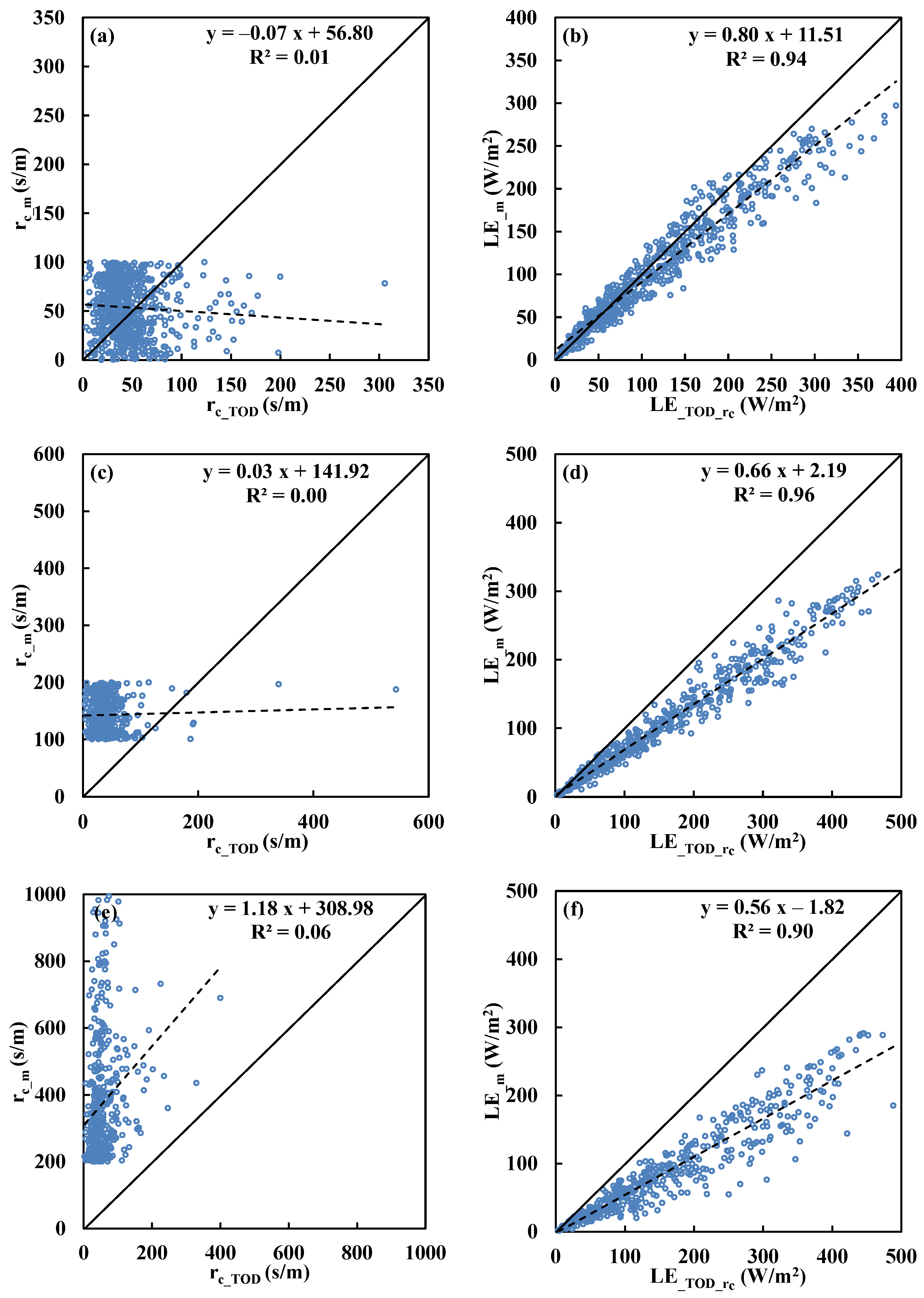
Figure 3.
Comparisons between measured canopy resistance (rc_m) and estimations by (a) SVM (rc_SVM) model and (b) Todorovic’s analytical solution (rc_TOD) above Dripsey grassland.
For the predictive trends, both methods tend to predict rc within specific ranges (the constant canopy resistance method uses fixed value). The SVM method has a wider prediction range, primarily falling within the range of 100 to 200 s/m. On the other hand, Todorovic’s analytical equation tends to predict very low canopy resistance values (mostly between 0–100 s/m), as explained in Equations (13) and (14). In other words, it can be inferred that Todorovic’s method tends to provide more accurate predictions of LE when dealing with smaller measured rc (rc < 100). However, when encountering medium to high measured rc, larger errors might occur.
4.2.2. Chi-Lan Forest
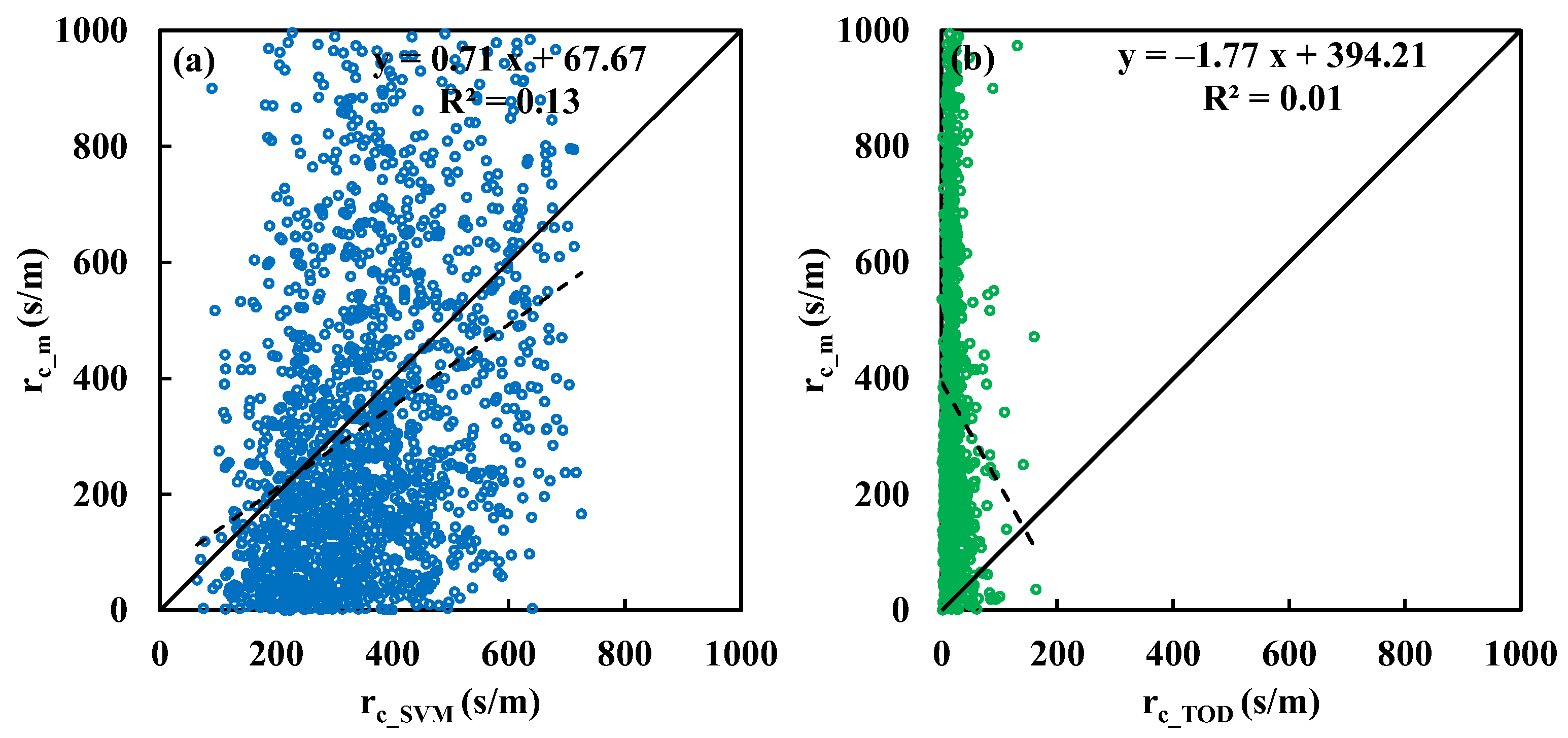
Table 4 presents the performance measures for estimated rc at the Chi-Lan forest. Figure 4 illustrates the comparison of measured and model-estimated rc in a 1:1 plot. From Table 4, both methods failed to reproduce rc well in the Chi-Lan forest. In terms of correlation, the R2 (=0.13) of the estimated rc using the SVM is even lower than that at the grassland. Similarly, the R2 for Todorovic’s analytical solution estimations is only 0.01. The RMSEs for the SVM and Todorovic’s methods are 248 and 425 s/m, respectively, with an average rc of 346 s/m at this Cypress forest.
Table 4.
Summary of linear regression between measured and model estimated canopy resistance (rc) and latent heat flux (LE) above Chi-Lan forest. rc_SVM and rc_TOD denote the rc estimated by SVM and Todorovic’s method, respectively; LE_SVM_rc, LE_TOD_rc, and LE_avg_rc denote the estimated LE where the rc is from SVM, Todorovic’s method, and the average, respectively. RMSE: root mean square error.

Figure 4.
Comparisons between measured canopy resistance (rc_m) and estimations by (a) SVM (rc_SVM) model and (b) Todorovic’s analytical solution (rc_TOD) above Chi-Lan forest.
Regarding to the predictive trend, the SVM method exhibits a broader range (150–600 s/m) of predicted rc values. On the other hand, Todorovic’s method tends to predict extremely low rc, with most of the predictions less than 75 s/m. The majority of predicted rc values from Todorovic’s method are below 50 s/m.
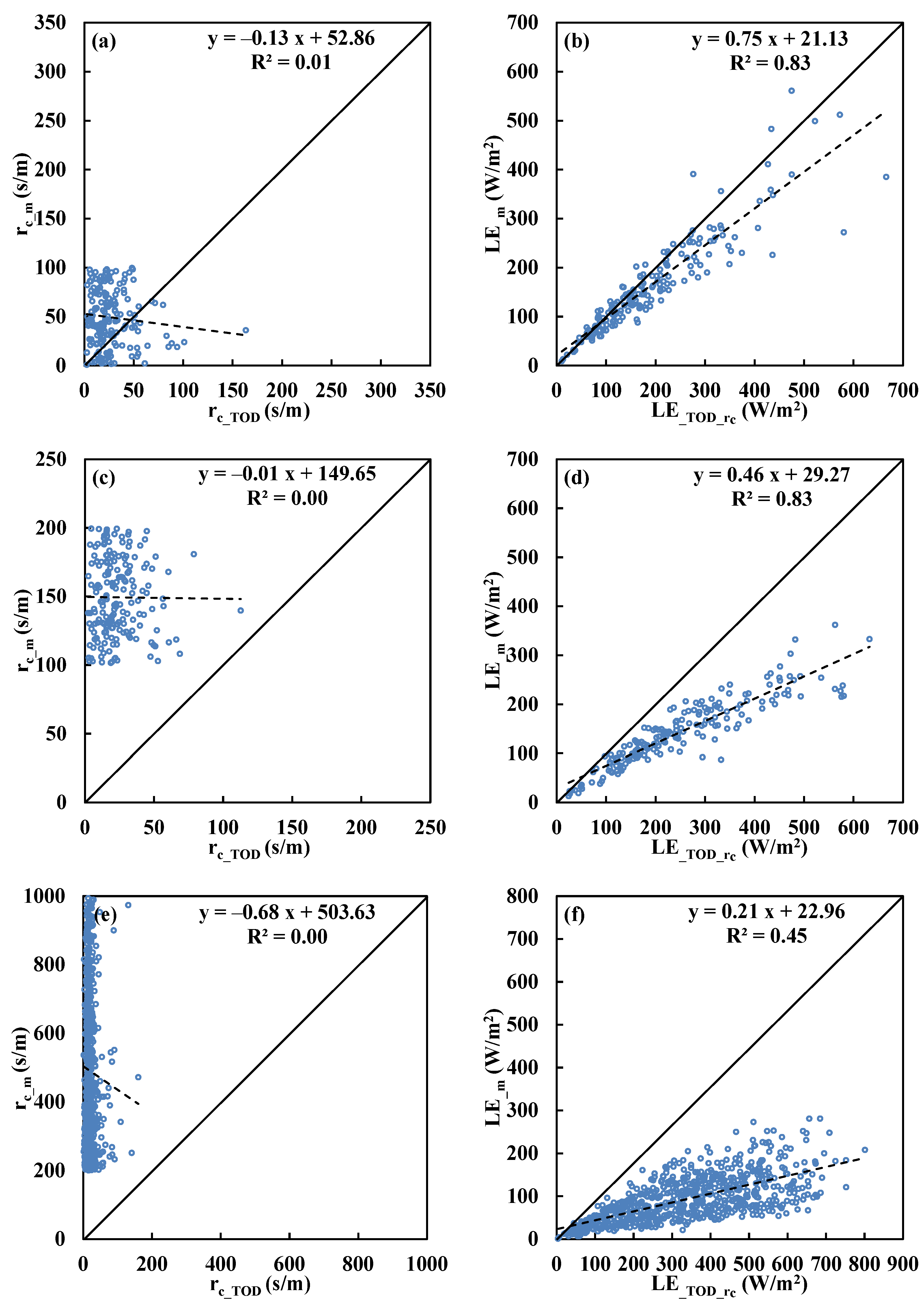
4.2.3. Sitou Forest
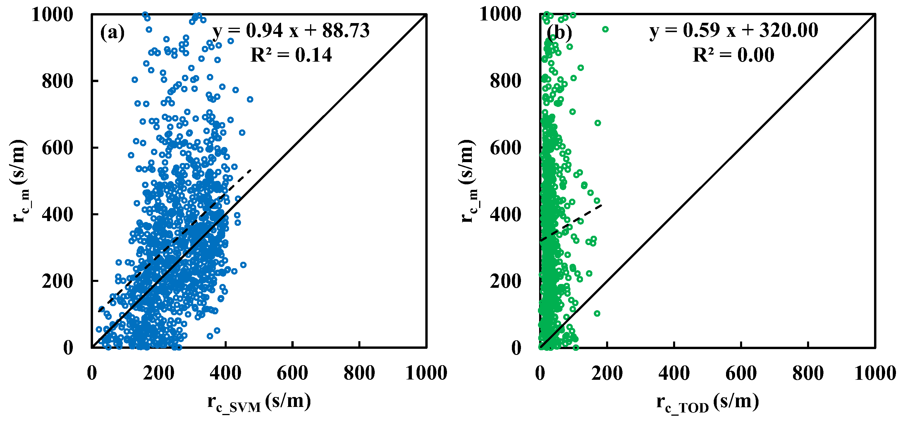
Table 5 summarizes the performance metrics for predicting rc in the Sitou forest, while Figure 5 illustrates the comparison of predictions against the measured rc in a 1:1 plot. From Table 5, the performances for rc prediction in the Sitou forest are quite similar to those in the Chi-Lan forest. Both methods failed to reproduce rc. At this Cryptomeria forest, the R2 value for rc prediction using the SVM method is 0.14, while Todorovic’s analytical solution predictions showed no correlation with the measurements (R2 = 0). The RMSEs of the SVM and Todorovic’s methods are 150 and 373 s/m, respectively, while the average rc for this site is 321 s/m.
Table 5.
Summary of linear regression between measured and model estimated canopy resistance (rc) and latent heat flux (LE) above Sitou forest. rc_SVM and rc_TOD denote the rc estimated by SVM and Todorovic’s method, respectively; LE_SVM_rc, LE_TOD_rc, and LE_avg_rc denote the estimated LE where the rc is from SVM, Todorovic’s method, and the average, respectively. RMSE: root mean square error.

Figure 5.
Comparisons between measured canopy resistance (rc_m) and estimations by (a) SVM (rc_SVM) model and (b) Todorovic’s analytical solution (rc_TOD) above Sitou forest.
In terms of the prediction range of rc, the SVM estimated rc ranged from 0 to 400 s/m. On the other hand, same as the grassland and Cypress forest sites, Todorovic’s method tends to predict low rc values (<100 s/m).
In summary, both the SVM and Todorovic’s methods do not provide accurate rc estimations, though Todorovic’s method works better at the grassland than the two forests. The failure of Todorovic’s analytical solution comes from the assumptions of this method, which were not satisfied above these three sites. The uncertainty of SVM estimations comes from the measured rc. Detail discussions are provided in Section 4.5 and Section 4.6.
4.3. Model Performance in Estimating LE
Figure 6, Figure 7 and Figure 8 show the comparisons between the observed and P–M equation predicted LE by the SVM, Todorovic’s analytical solution, and the constant canopy resistances. Although poor results for estimating rc, the estimated LE was in better agreement with the measurements. In the following sections, we will provide detailed explanations for the Dripsey grassland, Chi-Lan forest, and Sitou forest, respectively.
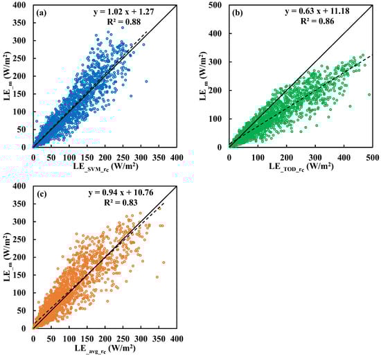
Figure 6.
Comparisons between measured latent heat flux (LE_m) and estimations by (a) SVM (LE_SVM_rc) model, (b) Todorovic’s analytical solution (LE_TOD_rc), and (c) constant rc (LE_avg_rc) above the Dripsey grassland.

Figure 7.
Comparisons between measured latent heat flux (LE_m) and estimations by (a) SVM (LE_SVM_rc) model, (b) Todorovic’s analytical solution (LE_TOD_rc), and (c) constant rc (LE_avg_rc) above Chi-Lan forest.
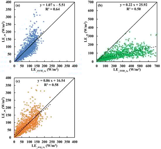
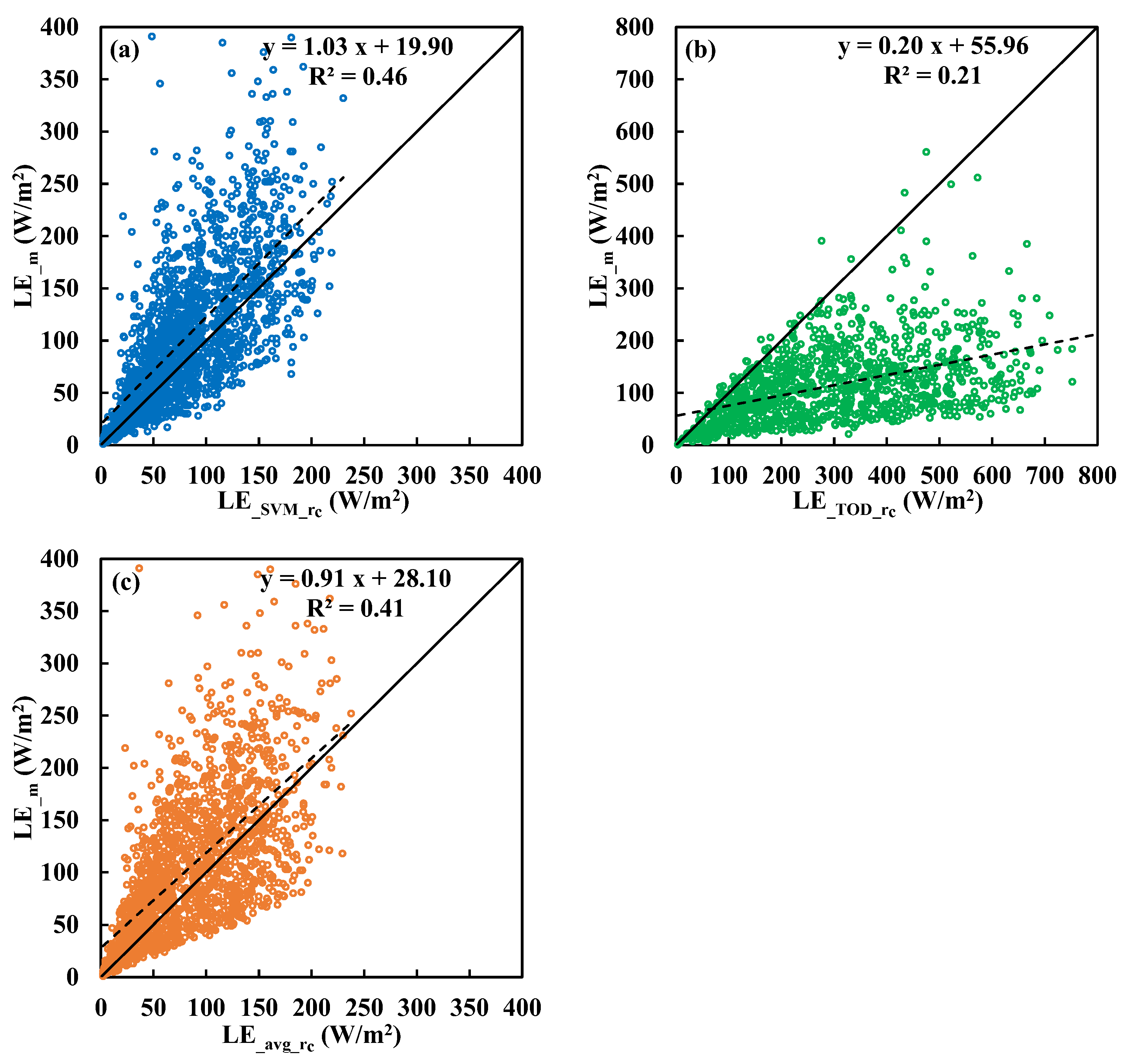
Figure 8.
Comparisons between measured latent heat flux (LE_m) and estimations by (a) SVM (LE_SVM_rc) model, (b) Todorovic’s analytical solution (LE_TOD_rc), and (c) constant rc (LE_avg_rc) above Sitou forest.
4.3.1. Dripsey Grassland
Figure 6 shows the comparisons between measured LE and P–M equation estimated LE using the rc values from the SVM, Todorovic’s analytical solution, and the constant (i.e., the average) canopy resistance at the grassland. The regression analyses between LE measurements and predictions are also summarized in Table 3. All LE predictions from the three methods are strongly correlated with the measurements (R2 = 0.83 to 0.88); however, Todorovic’s method tends to overestimate LE by 58.7% (slope = 0.63, see Table 3) and results in a high RMSE (=64 W/m2) while the other two methods’ RMSEs are less than 30 W/m2.
The overestimation of LE in Todorovic’s method is attributed to the following:
- (1)
- Surface energy imbalance. In this grassland, the energy closure rate is approximately 72% (H+LE is 72% of Qn). Hence, if we take this into account and force the energy to be closed, the ratio of measured LE to the estimated LE by Todorovic’s method combined with the P–M equation should be 87.5% (slope = 0.63/0.72 = 0.875); in other words, the overestimation rate is only 14%. In both the SVM and constant canopy resistance methods, since the training target values used for both methods are all based on the rc calculated from Equation (3), the energy imbalance in Equation (1) is compensated automatically.
- (2)
- The study area does not meet the assumption of Todorovic’s method. According to the assumption in Todorovic’s study [11], the pseudo resistance (r′) should be the same as the rc, that is, r′ = rc. However, this is not the case in Dripsey grassland. A detailed discussion is provided in Section 4.5.
4.3.2. Chi-Lan Forest
Figure 7 is the same as Figure 6 but for the Chi-Lan forest. The regression analyses between the measured and estimated LE are also summarized in Table 4. From Figure 7 and Table 4, the R2 between measured and estimated LE from the three methods are low: 0.46 (SVM), 0.21 (Todorovic), and 0.41 (constant rc); nevertheless, these low values are comparable to the R2 (=0.35) between measured LE and Qn (Figure 2d). Similar to the results at the grassland, Todorovic’s analytical solution overestimated LE (regression slope = 0.20) and resulted in a high RMSE (=233 W/m2), while the other two methods’ RMSEs are less than 60 W/m2 at this Cypress forest site. As indicated by Equation (14), Todorovic’s method is more suitable for environments with smaller measured rc, and in the Chi-Lan forest, the average rc (=346 s/m) is quite large, indicating that this Cypress forest is not suitable for the application of Todorovic’s method and thus exhibits larger errors. Even after taking into account the effect of energy imbalance (closure rate = 72%), the regression slope is still very low (0.20/0.72 = 0.278), showing a strong overestimation by Todorovic’s method.
Also, notice that in this forest site, the constant canopy resistance in conjunction with the P–M equation also slightly overestimated LE (Figure 7c, regression slope = 0.91). This implies that the average rc in the training dataset is slightly different from the average rc in the testing dataset. In other words, the average rc in this forest changed with time (seasons).
4.3.3. Sitou Forest
Figure 8 shows the comparisons between measured and predicted LE by P–M equation in conjunction with the rc from SVM, Todorovic, and constant canopy resistance methods at the Sitou forest. The performances of these three methods in this study area are quite similar to the results observed at the Chi-Lan forest (see regression summary in Table 5). From Table 5, the RMSE values obtained by the three methods range from 33.74 to 218.53 (W/m2), which are slightly lower than those in the Chi-Lan forest. The R2 values ranged from 0.50 (Todorovic) to 0.64 (SVM) and are comparable to the R2 (0.55) between measured LE and Qn (Figure 2f) at Sitou forest. Hence, the performance of the P–M equation in this Cryptomeria forest is better than that in the Chi-Lan forest (R2 = 0.20–0.46).
Again, Todorovic’s method systematically overestimated LE. After the correction for energy imbalance (closure rate = 52%), the regression slope is still low (0.22/0.52 = 0.423), showing a significant overestimation by Todorovic’s method.
Also, similar to the Chi-Lan forest, the constant canopy resistance in conjunction with the P–M equation also slightly overestimated LE (Figure 8c, regression slope = 0.86). This implies that the average rc in this Cryptomeria forest varied with time (seasons).
4.4. Model Performance in Different Ranges of Canopy Resistance
According to Lin et al. [6], the P–M equation exhibits varying sensitivity across different ranges of rc values. Particularly, it shows high sensitivity in the range of rc = 0–100 (s/m), medium sensitivity in the range of 100–200 (s/m), and low sensitivity for rc larger than 200 (s/m). Since Todorovic’s analytical solution tends to produce a small rc, it can be inferred that with smaller measured rc values (rc < 100), the error between LE estimations and measurements would be smaller. However, when encountering situations with larger measured rc, significant errors would occur and lead to a decrease in the overall model performance. In this section, we compiled the performance metrics of SVM and Todorovic’s methods for the above three sensitivity ranges at the three study sites.
Table 6 summarizes the model performances for estimating canopy resistance and LE in the high (rc: 0–100 s/m), medium (rc: 100–200 s/m), and low (rc > 200 s/m) sensitivity ranges above the Dripsey grassland. From the analysis of rc estimations in Section 4.2, it was noticed that both SVM and Todorovic’s methods tend to produce rc within a certain interval. Therefore, at this grassland, as the SVM tends to reproduce rc in the medium range (where the RMSE for estimated rc is the smallest among the three ranges), the RMSE (=21.59 W/m2) of LE estimation in this interval is then the lowest compared with the high sensitivity interval (RMSE = 27.25 W/m2) and the low sensitivity interval (RMSE = 27.66 W/m2).
Table 6.
Summary of linear regression between measured and model estimated canopy resistance (rc) and latent heat flux (LE) above Dripsey grassland for three different ranges (0–100, 100–200, and >200) of measured canopy resistance (rc_m). rc_SVM and rc_TOD denote the rc estimated by SVM and Todorovic’s method, respectively; LE_SVM_rc and LE_TOD_rc the estimated LE where the rc is from SVM and Todorovic’s method, respectively. RMSE: root mean square error; Int.: intercept.
On the other hand, Todorovic’s method tends to predict rc within the high sensitivity interval; therefore, the RMSE of predicted LE in the high sensitivity interval is also the lowest (26.32 W/m2) compared with the other two intervals. As the measured rc increases to the medium and low sensitivity intervals, the RMSE of LE predictions also increases to 70 and 90 (W/m2), respectively. Detailed scatter plots of LE v.s. Rn–G and comparisons between measurements and predictions of rc and LE by SVM and Todorovic’s methods for these three intervals at the Dripsey grassland are presented in Appendix A.1.
Table 7 is the same as Table 6 but for the Chi-Lan forest. In this forest, Todorovic’s method also tends to predict rc more accurately in the high sensitivity interval, resulting in the lowest error of LE estimations with an RMSE of 55.48 (W/m2). However, as rc_m increases to the medium and high sensitivity intervals, the RMSE significantly rises to 132 and 279 (W/m2), respectively. On the contrary, due to being trained by historical data, the SVM tends to predict rc mainly ranging from 150 to 600 (s/m), with maximum values reaching around 750 (s/m). It is observed that the SVM method achieves the lowest RMSE in the low sensitivity interval (=32.87 W/m2). As rc_m decreases to medium or high sensitivity intervals, the errors in predicting LE also increase to 60 and 91 (W/m2), respectively. Noticed that, for the SVM model, the best rc estimation is in the medium range; however, the best LE estimation is in the low sensitivity range. This is because, in the low range, the LE estimation is not sensitive to the rc value [6].
Table 7.
Summary of linear regression between measured and model estimated canopy resistance (rc) and latent heat flux (LE) above Chi-Lan forest for three different ranges (0–100, 100–200, and >200) of measured canopy resistance (rc_m). rc_SVM and rc_TOD denote the rc estimated by SVM and Todorovic’s method, respectively; LE_SVM_rc and LE_TOD_rc the estimated LE where the rc is from SVM and Todorovic’s method, respectively. RMSE: root mean square error; Int.: intercept.
Table 8 is the same as Table 6 but for the Sitou forest. Although both the Chi-Lan and Sitou areas belong to the foggy mountain forest, and the errors for LE estimations are quite similar, there is a notable difference in coefficients of determination (R2) between the two sites. From Table 7 and Table 8, in all three intervals, the R2 values for LE estimations by the SVM model are higher (0.77–0.89) at the Sitou forest and smaller (0.64–0.76) at the Chi-Lan forest. The same results are found in the LE estimations by Todorovic’s analytical solution. This phenomenon can be explained by noting that the correlation between LE and Rn–G is higher at the Sitou forest site. From Figure 2, Figure A1, Figure A4 and Figure A7, it is evident that the correlation between LE and Rn–G determines the R2 between LE measurements and estimates by the P–M equation. This is because the P–M equation uses Rn–G to estimate LE.
Table 8.
Summary of linear regression between measured and model estimated canopy resistance (rc) and latent heat flux (LE) above Sitou forest for three different ranges (0–100, 100–200, and >200) of measured canopy resistance (rc_m). rc_SVM and rc_TOD denote the rc estimated by SVM and Todorovic’s method, respectively; LE_SVM_rc and LE_TOD_rc the estimated LE where the rc is from SVM and Todorovic’s method, respectively. RMSE: root mean square error; Int. intercept.
Also, same as the Chi-Lan forest site, noticed that, for the SVM model, the best rc estimation is in the medium range; however, the best LE estimation is in the low sensitivity range. Detailed scatter plots of LE v.s. Rn–G and comparisons between measured and predicted rc and LE by SVM and Todorovic’s methods for these three intervals at the Chi-Lan forest and Sitou forest are provided in Appendix A.2 and Appendix A.3, respectively.
4.5. Uncertainty of Todorovic’s Analytical Solution
To investigate why Todorovic’s approach did not work, we have to check the following two assumptions (arguments) made in this method: (1) whether r’ can be represented by rc? (2) if the approximation for t, i.e., Equation (6), is valid?
By replacing r′ with rc, Equation (5) becomes
where H′ by Equation (4) is expressed as
In conjunction with Equation (16) and measured LE, Qn, and rc, Equation (15) provides an analytical solution for t (canopy temperature increase). Now by substituting Equation (6) into Equation (5), we have
In conjunction with Equation (16) and measured LE and Qn, Equation (17) provides an analytical solution for r′.
Using the mean measured LE, Qn, and rc, Figure 9a shows the t comparison between Todorovic’s expression (tTOD, i.e., Equation (6)) and the analytical solution (tana, i.e., Equation (15)) at the Dripsey grassland. It is clear from Figure 9a that the t value obtained from Todorovic’s expression is systematically lower than the t value required from the analytical solution. This indicates that if r′ = rc, then Todorovic’s expression (i.e., Equation (6)) for t is not valid at this grassland.
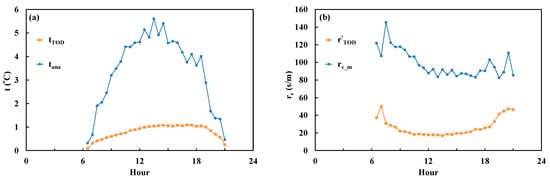
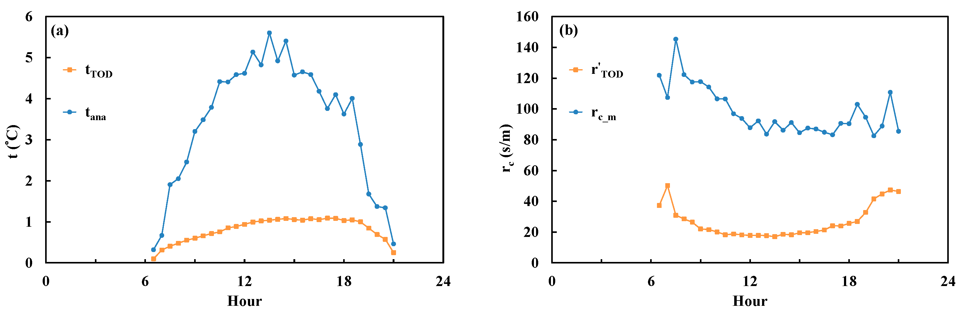
Figure 9.
Comparisons between (a) canopy temperature increase calculated by Todorovic’s expression (tTOD, Equation (6)) and the analytical solution (tana, Equation (16)); (b) pseudo resistance (r’TOD, calculated by Equation (17)) and measured canopy resistance (rc_m, calculated by Equation (3)) above Dripsey grassland.
Using the mean measured LE, Qn, and t from Todorovic’s expression (i.e., Equation (6)), Figure 9b shows the comparison between r′ (calculated from Equation (17)) and rc (calculated from Equation (3)). It is clear that r′ is much smaller than the measured rc in Figure 9b. The measured rc during the early morning period was around 100 (s/m) and maintained around 90 (s/m) for the noon and afternoon periods. In contrast, the r’ was only about 20 (s/m) for most of the daytime. This indicates that if Todorovic’s expression (i.e., Equation (6)) is valid, then the assumption of r′ = rc is not satisfied at this grassland. Notice that the rc_m in Figure 9b is different from the rc_m in Figure 1a, where rc_m is first calculated by Equation (3) for each data and then averaged.
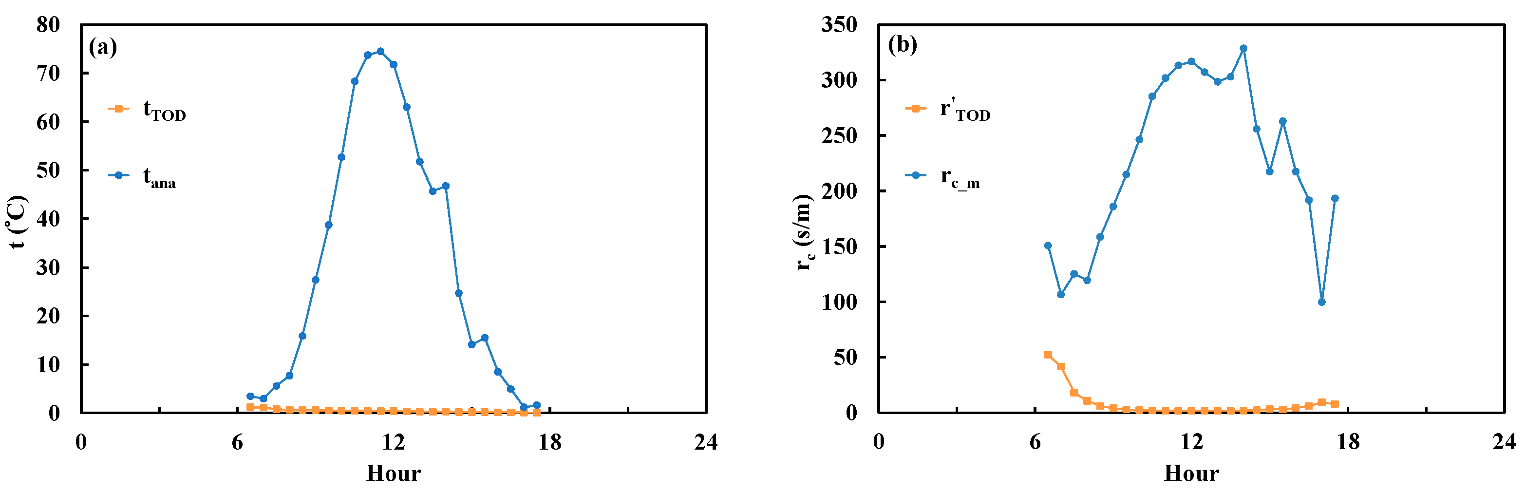
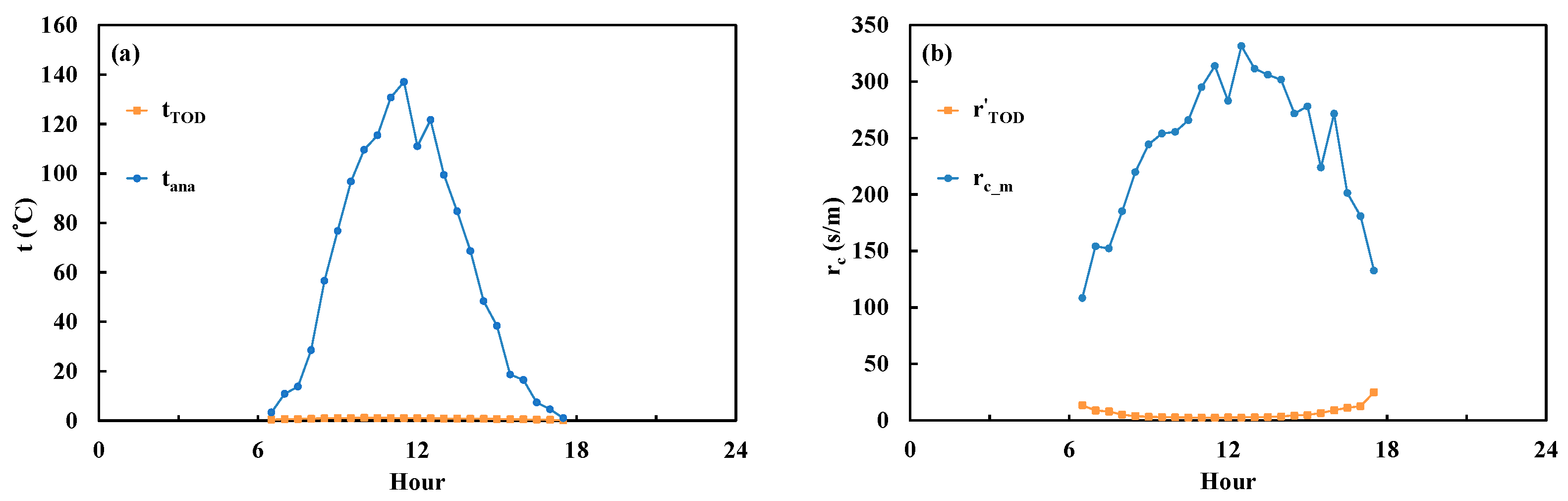
Figure 10 is the same as Figure 9 but for the Chi-Lan forest. As shown in Figure 10a, within this forest, the theoretical temperature increase in the canopy (tana) calculated from Equation (16) was very high and not reasonable (maximum = 74.52 °C at 11:30); this high value of t resulted from the high value of rc at this site and assuming r’ = rc. However, the t values calculated using the approximation proposed by Todorovic are small (maximum around 1 °C) and similar to those in the grassland.
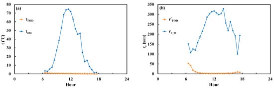
Figure 10.
Comparisons between (a) canopy temperature increase calculated by Todorovic’s expression (tTOD, Equation (6)) and the analytical solution (tana, Equation (16)); (b) pseudo resistance (r’TOD, calculated by Equation (17)) and measured canopy resistance (rc_m, calculated by Equation (3)) above Chi-Lan forest.
Figure 10b illustrates that, for the Chi-Lan forest, r′ is very different from rc and is much smaller. The disagreement between r′ and rc_m for this Cypress forest is much larger than that observed in the Dripsey grassland, which further indicates that Todorovic’s analytical solution for rc is not suitable for this forest site.
Figure 11 is the same as Figure 9 but for the Sitou forest. The trends of tTOD and tana in Figure 11a are quite similar to those in Figure 10a, but the maximum tana (around 140 °C) is even higher than that in the Chi-Lan forest; part of this is caused by the larger energy imbalance at the Sitou forest. As to the comparison between r′ and rc, similar results to those in Chi-Lan Forest were also found in Sitou Forest (Figure 11b). Figure 11a,b demonstrates that Todorovic’s method is not suitable for this Cryptomeria forest.
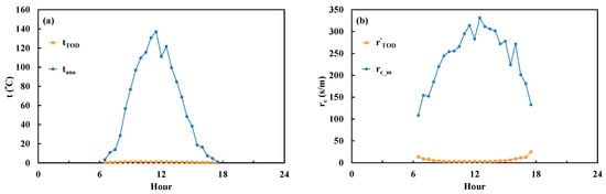
Figure 11.
Comparisons between (a) canopy temperature increase calculated by Todorovic’s expression (tTOD, Equation (6)) and the analytical solution (tana, Equation (16)); (b) pseudo resistance (r’TOD, calculated by Equation (17)) and measured canopy resistance (rc_m, calculated by Equation (3)) above Sitou forest.
4.6. Uncertainty of the P–M Equation, Support Vector Machine, and Constant Canopy Resistance
The uncertainty of SVM for estimating rc mainly comes from the measured rc for training the SVM model. From Equation (3), the canopy resistance is a function of available radiation energy, LE, air temperature, wind speed, and vapor pressure deficit. In Appendix B we plotted measured rc as a function of these meteorological variables for Dripsey grassland, Chi-Lan forest, and Sitou forest, respectively. From Appendix B, it is clear that rc spreads out a lot with the meteorological variables; this explains why the SVM model was not able to predict rc well.
From Equation (1), it is clear that the major uncertainty of the P–M equation for estimating LE comes from the surface energy imbalance. However, since the measured rc in this study was calculated from the reverse of Equation (1), i.e., Equation (3), the energy imbalance portion has been taken into account in the SVM and constant canopy resistance methods (recall: the SVM model were trained by the historical observed rc; the constant canopy resistance method takes the average of the historical observed rc as the constant rc). However, the LE calculated from the rc estimated by Todorovic’s analytical solution would suffer from this energy imbalance problem. From Figure 2, Table 3, Table 4 and Table 5, and Appendix A, it is evident that the R2 between measured and predicted LE depends on the correlation of measured LE v.s. Rn–G, and not sensitive to the accuracy of rc estimation; also, from Table 3, Table 4, Table 5, Table 6, Table 7 and Table 8, the RMSE of LE estimation depends on the accuracy of rc.
To investigate the errors caused by the surface energy imbalance from Todorovic’s method, we calculated the percentage error for the three sites. The percentage errors are 47.5%, 194.1%, and 244.8% for Dripsey grassland, Chi-Lan forest, and Sitou forest, respectively. The energy closure rates are 72%, 72%, and 52% for Dripsey grassland, Chi-Lan forest, and Sitou forest, respectively. After forcing the surface energy to be closed, in other words, the available energy, Qn, in Equation (3) is replaced by H+LE; then the percentage errors are 6.2%, 111.8%, 79.3%, respectively.
5. Conclusions
In this study, two methods (Support Vector Machine and Todorovic’s analytical solution) are used to estimate the canopy resistances of a grassland and two forests. These estimated canopy resistances were then applied in the P–M equation for estimating ET; as a benchmark, a constant canopy resistance was also adopted for ET estimations. Our results demonstrate the following:
- (1)
- The estimated rc from Todorovic’s analytical solution exhibits no correlation with the observed rc. On the other hand, the support vector machine’s rc estimation is slightly better, with R2 values ranging between 0.13 and 0.22 across the three research areas. Both methods tend to reproduce the canopy resistances within a certain range of intervals.
- (2)
- Contrary to rc estimations, the LE estimations are in better agreement with the observations when the estimated rc are adopted in the Penman–Monteith equation. In general, the SVM model performs better than the analytical solution.
- (3)
- The failure of the analytical solution in estimating rc is attributed to the assumption of r′ = rc. Using this method will lead to a significant underestimation of canopy resistance and subsequently an overestimation of latent heat flux. This discrepancy is more obvious in forests where rc is in a bigger value (around 320 s/m).
- (4)
- The coefficient of determination (R2) of regression between the measured and P–M equation estimated LE is strongly dependent on the correlation between measured LE and available energy (Rn–G) and not sensitive to the accuracy of rc estimation; however, the RMSE of LE estimation depends on the accuracy of rc.
If there is sufficient and reliable on-site measurement data, the machine learning method would be a better approach for estimating canopy resistance. When data availability is limited, considering the site vegetation condition becomes crucial. If the site is humid and covered with low canopy resistance vegetation (e.g., grassland), Todorovic’s analytical solution can be considered for estimating canopy resistance.
Author Contributions
C.-I.H. conceived the research idea; C.-I.H., C.-T.L. and I.-H.H. performed the analytical model simulations; C.-I.H. designed the input factors of machine learning approach. I.-H.H. performed the machine learning model simulations; C.-I.H. performed the Chi-Lan and Sitou forest experiments; all authors took part in the discussion, data analysis, and interpretation of the data and model estimations; C.-I.H., I.-H.H. and C.-T.L. wrote the manuscript. C.-I.H. finalized the manuscript. All authors have read and agreed to the published version of the manuscript.
Funding
This work was supported, in part, by the Ministry of Science and Technology, Taiwan [grant number: MOST 111-2111-M-002-010] and the Core Research Project, National Taiwan University [project number: NTU-CC-112L900504; NTU-CC-112L7452].
Data Availability Statement
The data used to support the findings of this study are available from the corresponding author upon request.
Acknowledgments
The Chi-Lan forest data used for this study were from the project by YJ Hsia, SC Chang, and CI Hsieh under the contracts with Environmental Protection Agency, Taiwan (EPA-94-L105-02-201 and EPA-96-FA11-03-A027-2). The authors are grateful to Shih-Min Cheng for her great help with the Sitou forest experiment. The grassland data were supported by G. Kiely, University College Cork, Ireland. The authors would like to thank the support received from Professor Yu-Li Wang and the Agricultural Net-Zero Carbon Technology and Management Innovation Research Center at National Taiwan University.
Conflicts of Interest
The authors declare no conflict of interest.
Appendix A. Energy Closure and Latent Heat Flux Estimations in Different Canopy Resistance Intervals
Appendix A.1. Dripsey Grassland Experiment
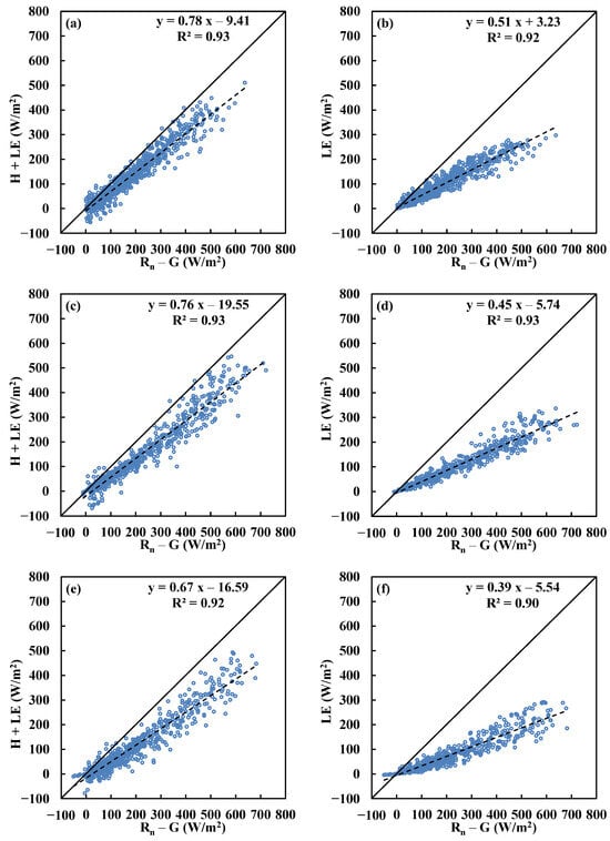
Figure A1.
Comparisons of H+LE v.s. Rn–G and LE v.s. Rn–G under different ranges of measured canopy resistance (rc): (a,b) rc < 100 (s/m), (c,d) rc =100–200 (s/m), and (e,f) rc > 200 (s/m) above Dripsey grassland.
Figure A1.
Comparisons of H+LE v.s. Rn–G and LE v.s. Rn–G under different ranges of measured canopy resistance (rc): (a,b) rc < 100 (s/m), (c,d) rc =100–200 (s/m), and (e,f) rc > 200 (s/m) above Dripsey grassland.

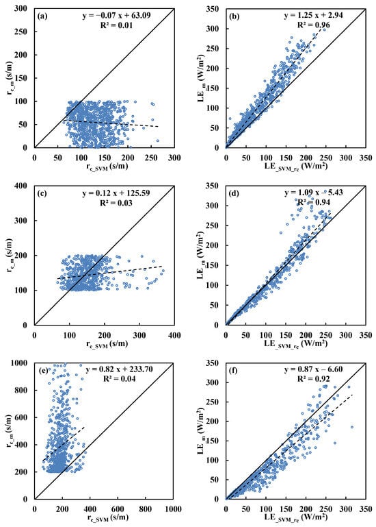
Figure A2.
Comparisons of measured canopy resistance (rc_m) and latent heat flux (LE_m) with estimations by SVM model (rc_svm, LE_SVM_rc) under different ranges of measured canopy resistance (rc): (a,b) rc < 100 (s/m), (c,d) rc =100–200 (s/m), and (e,f) rc > 200 (s/m) above Dripsey grassland.
Figure A2.
Comparisons of measured canopy resistance (rc_m) and latent heat flux (LE_m) with estimations by SVM model (rc_svm, LE_SVM_rc) under different ranges of measured canopy resistance (rc): (a,b) rc < 100 (s/m), (c,d) rc =100–200 (s/m), and (e,f) rc > 200 (s/m) above Dripsey grassland.
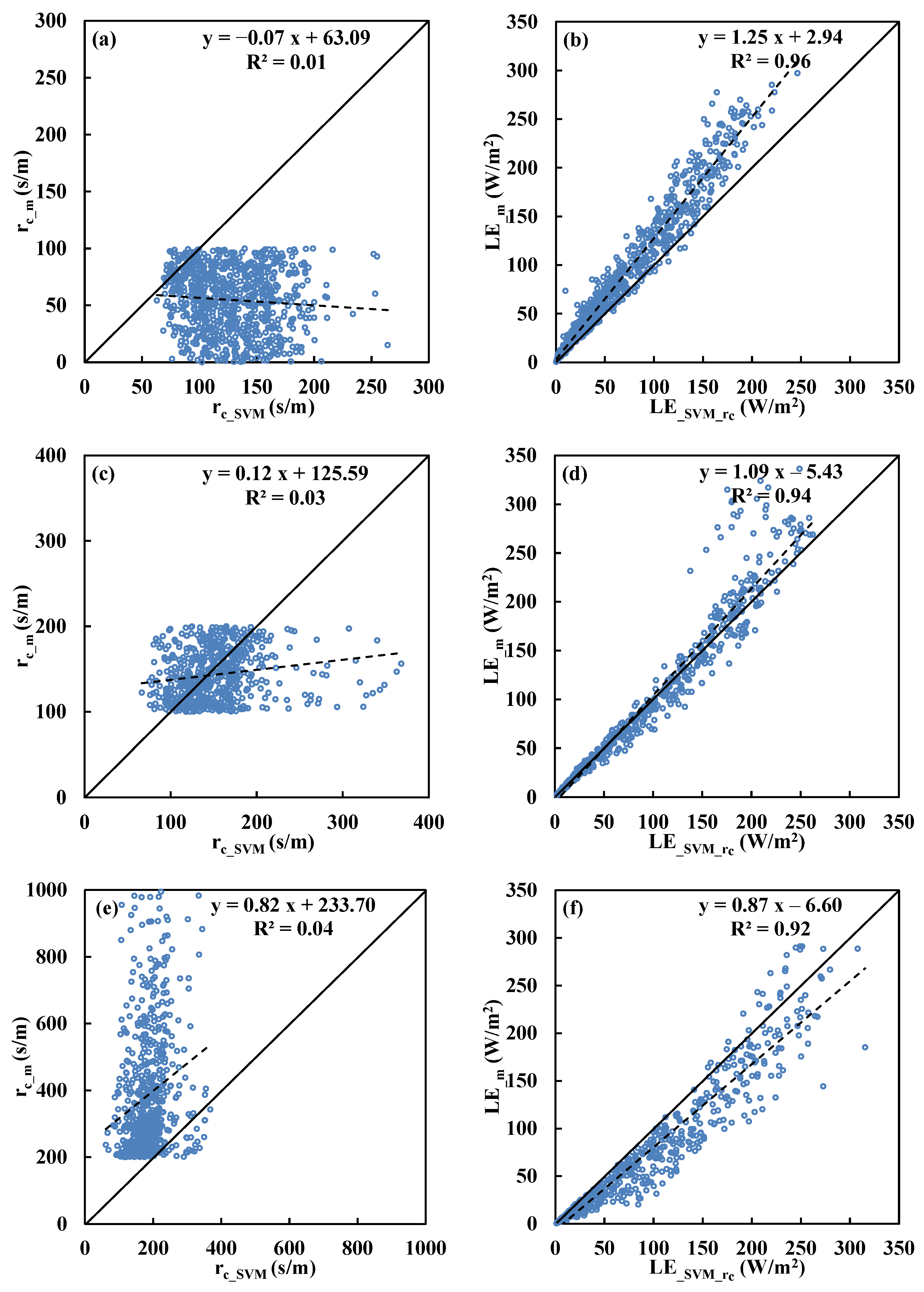
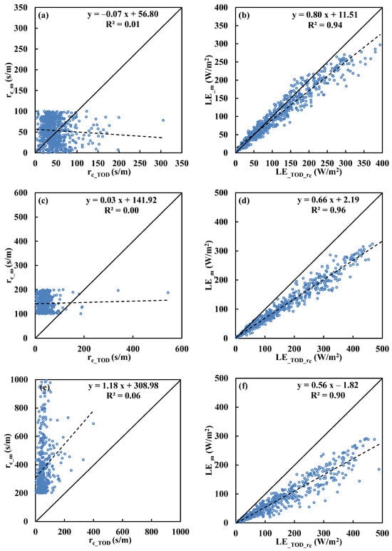
Figure A3.
Comparisons of measured canopy resistance (rc_m) and latent heat flux (LE_m) with estimations by Todorovic’s method (rc_TOD, LE_TOD_rc) under different ranges of measured canopy resistance (rc): (a,b) rc < 100 (s/m), (c,d) rc = 100–200 (s/m), and (e,f) rc > 200 (s/m) above Dripsey grassland.
Appendix A.2. Chi-Lan Forest Experiment
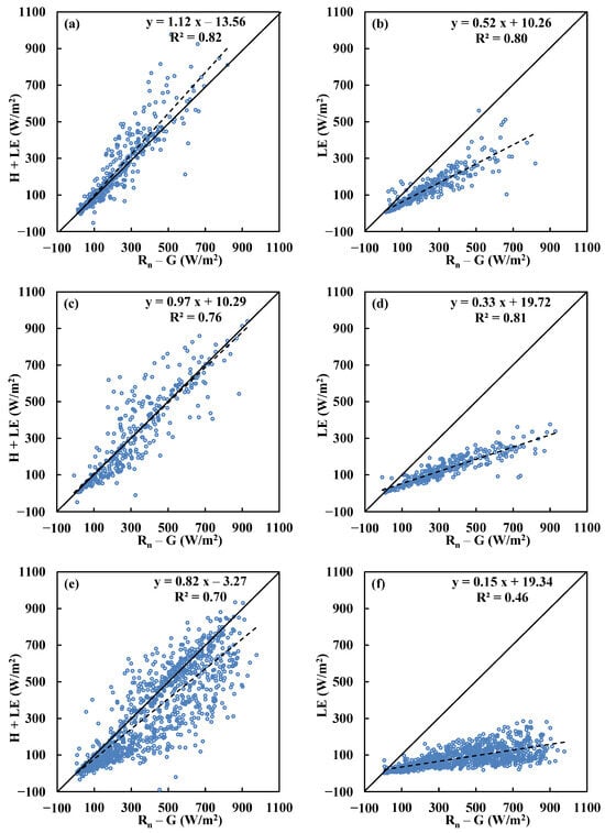
Figure A4.
Comparisons of H+LE v.s. Rn–G and LE v.s. Rn–G under different ranges of measured canopy resistance (rc): (a,b) rc < 100 (s/m), (c,d) rc = 100–200 (s/m), and (e,f) rc > 200 (s/m) above Chi-Lan forest.
Figure A4.
Comparisons of H+LE v.s. Rn–G and LE v.s. Rn–G under different ranges of measured canopy resistance (rc): (a,b) rc < 100 (s/m), (c,d) rc = 100–200 (s/m), and (e,f) rc > 200 (s/m) above Chi-Lan forest.
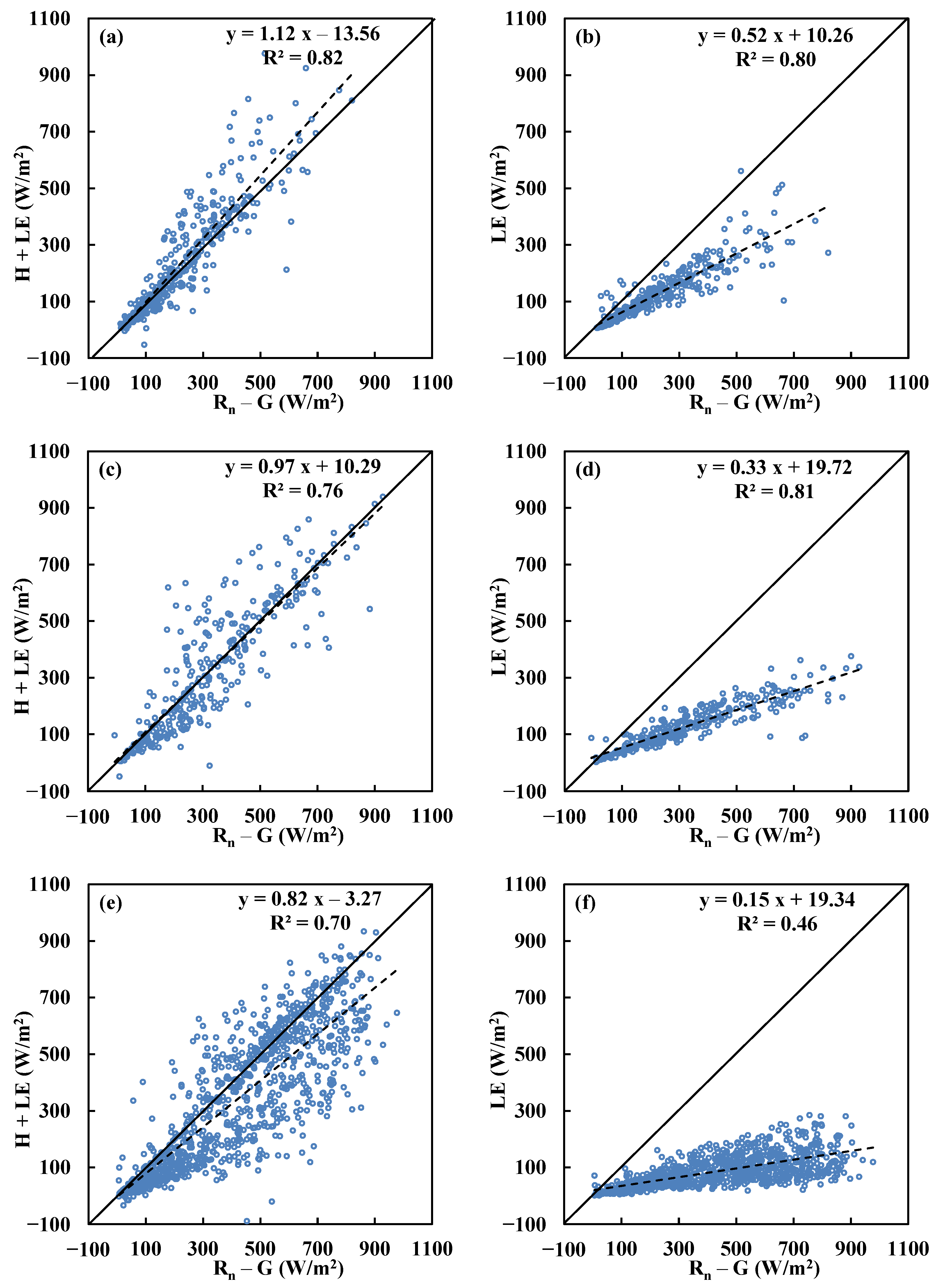
Figure A5.
Comparisons of measured canopy resistance (rc_m) and latent heat flux (LE_m) with estimations by SVM model (rc_svm, LE_SVM_rc) under different ranges of measured canopy resistance (rc): (a,b) rc < 100 (s/m), (c,d) rc = 100–200 (s/m), and (e,f) rc > 200 (s/m) above Chi-Lan mountain.
Figure A5.
Comparisons of measured canopy resistance (rc_m) and latent heat flux (LE_m) with estimations by SVM model (rc_svm, LE_SVM_rc) under different ranges of measured canopy resistance (rc): (a,b) rc < 100 (s/m), (c,d) rc = 100–200 (s/m), and (e,f) rc > 200 (s/m) above Chi-Lan mountain.
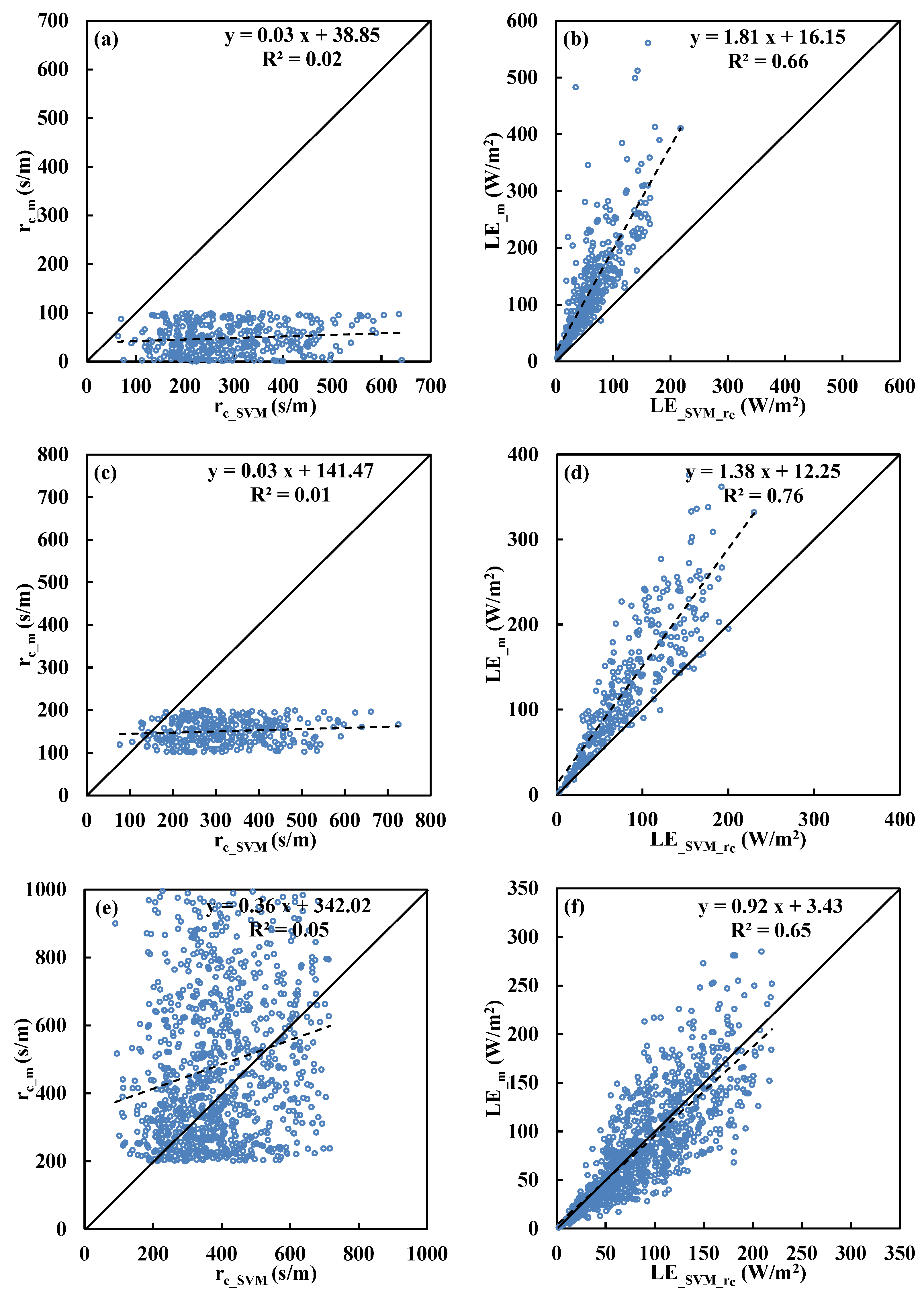

Figure A6.
Comparisons of measured canopy resistance (rc_m) and latent heat flux (LE_m) with estimations by Todorovic’s method (rc_TOD, LE_TOD_rc) under different ranges of measured canopy resistance (rc): (a,b) rc < 100 (s/m), (c,d) rc = 100–200 (s/m), and (e,f) rc > 200 (s/m) above Chi-Lan forest.
Appendix A.3. Sitou Forest Experiment
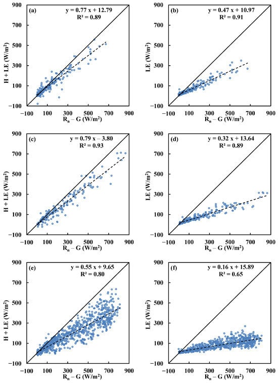
Figure A7.
Comparisons of H+LE v.s. Rn–G and LE v.s. Rn–G under different ranges of measured canopy resistance (rc): (a,b) rc < 100 (s/m), (c,d) rc = 100–200 (s/m), and (e,f) rc > 200 (s/m) above Sitou forest.
Figure A7.
Comparisons of H+LE v.s. Rn–G and LE v.s. Rn–G under different ranges of measured canopy resistance (rc): (a,b) rc < 100 (s/m), (c,d) rc = 100–200 (s/m), and (e,f) rc > 200 (s/m) above Sitou forest.

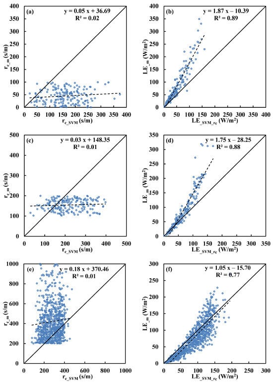
Figure A8.
Comparisons of measured canopy resistance (rc_m) and latent heat flux (LE_m) with estimations by SVM model (rc_svm, LE_SVM_rc) under different ranges of measured canopy resistance (rc): (a,b) rc < 100 (s/m), (c,d) rc = 100–200 (s/m), and (e,f) rc > 200 (s/m) above the Sitou forest.
Figure A8.
Comparisons of measured canopy resistance (rc_m) and latent heat flux (LE_m) with estimations by SVM model (rc_svm, LE_SVM_rc) under different ranges of measured canopy resistance (rc): (a,b) rc < 100 (s/m), (c,d) rc = 100–200 (s/m), and (e,f) rc > 200 (s/m) above the Sitou forest.

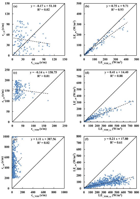
Figure A9.
Comparisons of measured canopy resistance (rc_m) and latent heat flux (LE_m) with estimations by Todorovic’s method (rc_TOD, LE_TOD_rc) under different ranges of measured canopy resistance (rc): (a,b) rc < 100 (s/m), (c,d) rc = 100–200 (s/m), and (e,f) rc > 200 (s/m) above the Sitou forest.

Appendix B. Scatter Plots of Canopy Resistance and Meteorological Variables
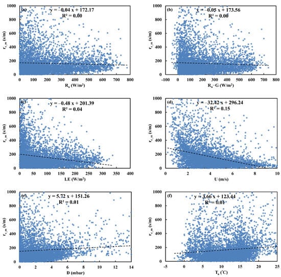
Figure A10.
Scatter plots of measured canopy resistance (rc_m) as a function of (a) net radiation (Rn), (b) available energy (Rn–G), (c) latent heat flux (LE), (d) wind speed (U), (e) vapor pressure deficit (D), and (f) air temperature (Ta) above Dripsey grassland.
Figure A10.
Scatter plots of measured canopy resistance (rc_m) as a function of (a) net radiation (Rn), (b) available energy (Rn–G), (c) latent heat flux (LE), (d) wind speed (U), (e) vapor pressure deficit (D), and (f) air temperature (Ta) above Dripsey grassland.
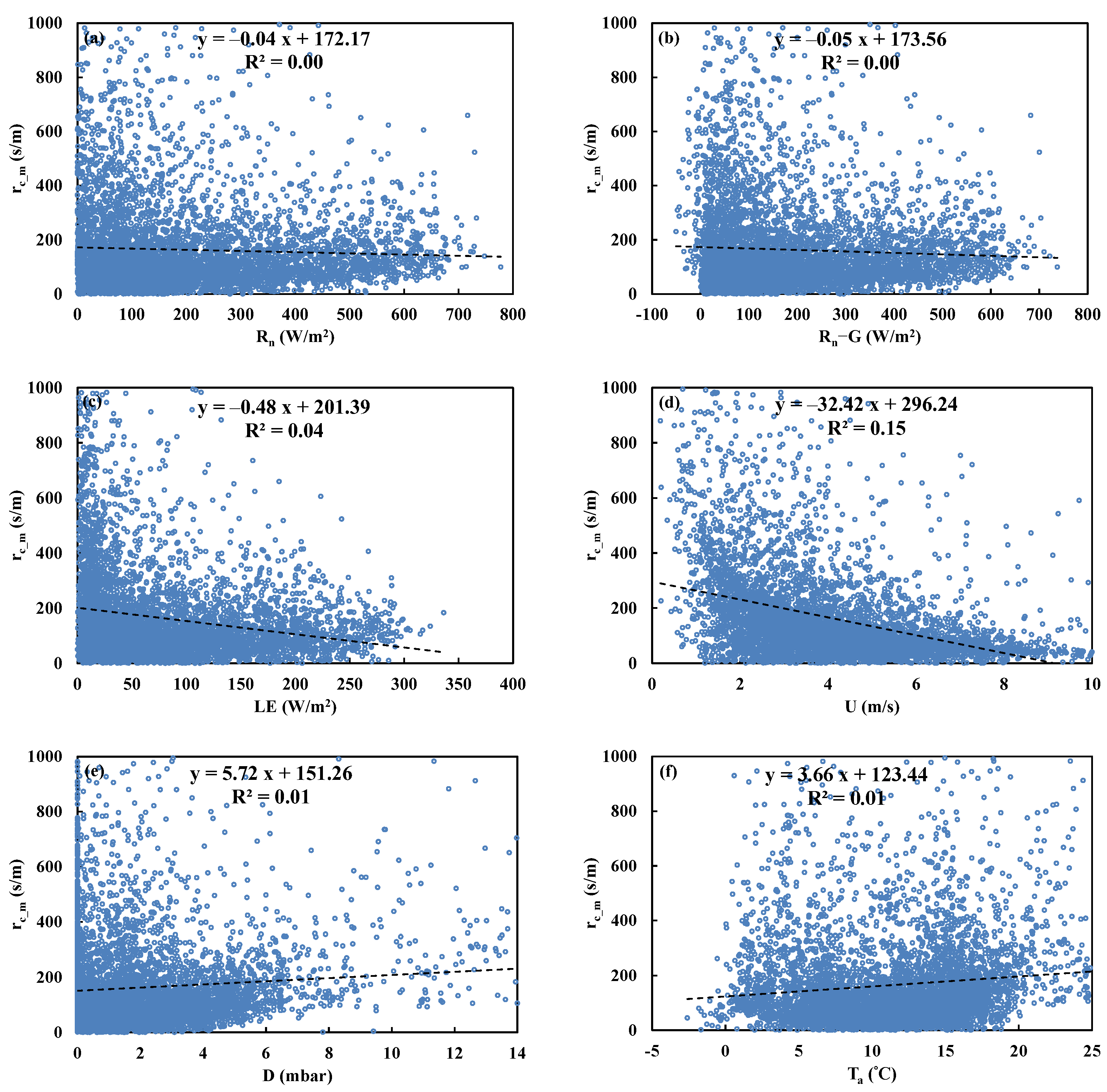
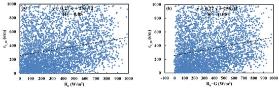

Figure A11.
Scatter plots of measured canopy resistance (rc_m) as a function of (a) net radiation (Rn), (b) available energy (Rn–G), (c) latent heat flux (LE), (d) wind speed (U), (e) vapor pressure deficit (D), and (f) air temperature (Ta) above Chi-Lan forest.
Figure A11.
Scatter plots of measured canopy resistance (rc_m) as a function of (a) net radiation (Rn), (b) available energy (Rn–G), (c) latent heat flux (LE), (d) wind speed (U), (e) vapor pressure deficit (D), and (f) air temperature (Ta) above Chi-Lan forest.
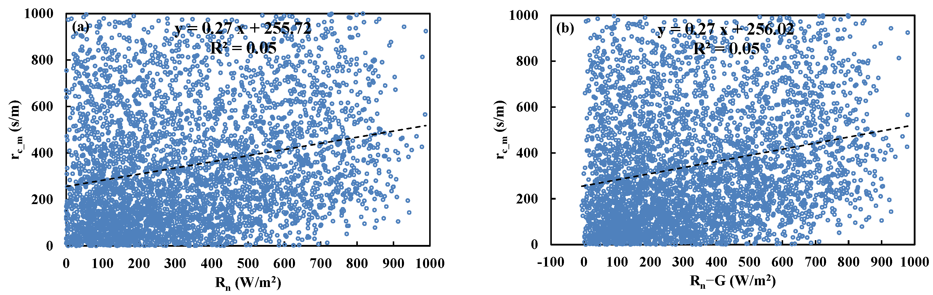
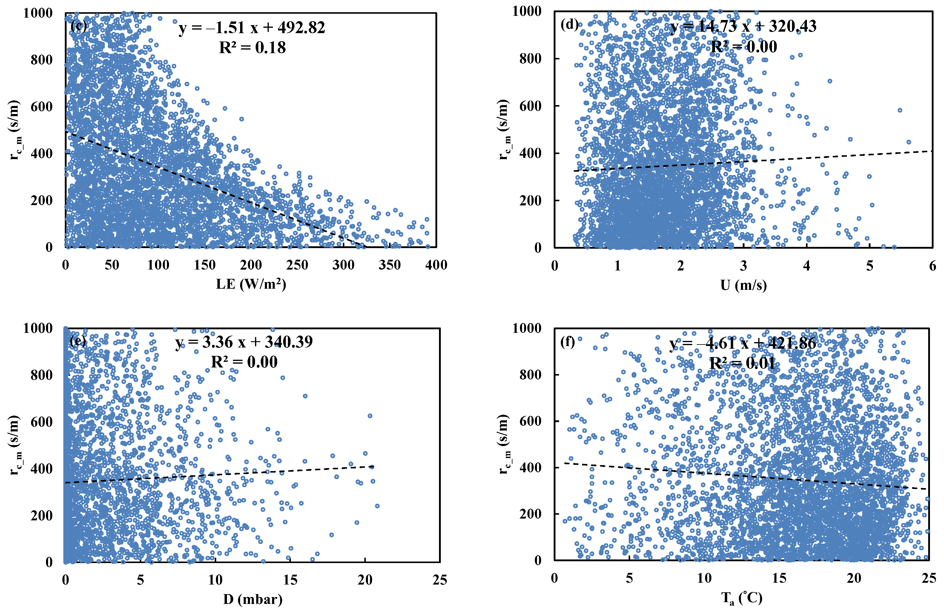
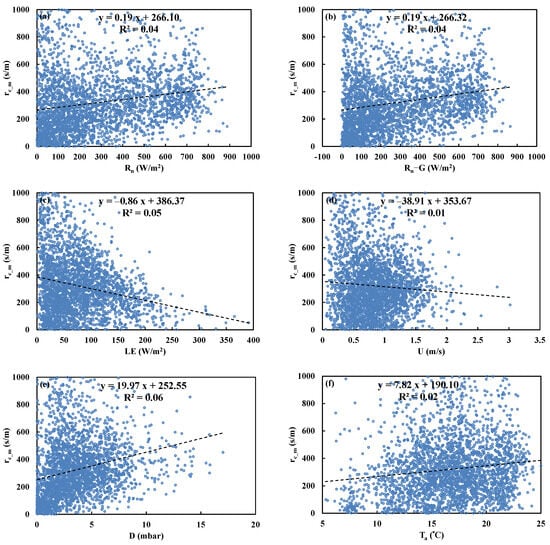
Figure A12.
Scatter plots of measured canopy resistance (rc_m) as a function of (a) net radiation (Rn), (b) available energy (Rn–G), (c) latent heat flux (LE), (d) wind speed (U), (e) vapor pressure deficit (D), and (f) air temperature (Ta) above Sitou forest.
Figure A12.
Scatter plots of measured canopy resistance (rc_m) as a function of (a) net radiation (Rn), (b) available energy (Rn–G), (c) latent heat flux (LE), (d) wind speed (U), (e) vapor pressure deficit (D), and (f) air temperature (Ta) above Sitou forest.

References
- Allen, R.G.; Pereira, L.S.; Raes, D.; Smith, M. Crop Evapotranspiration-Guidelines for Computing Crop Water Requirements-FAO Irrigation and Drainage Paper 56; FAO: Rome, Italy, 1998; ISBN 92-5-104219-5. [Google Scholar]
- Fisher, J.B.; Tu, K.P.; Baldocchi, D.D. Global estimates of the land-atmosphere water flux based on monthly AVHRR and ISLSCP-II data, validate at 16 FLUXNET sites. Remote Sens. Environ. 2008, 112, 901–919. [Google Scholar] [CrossRef]
- Sheffield, J.; Wood, E.F.; Munoz-Ariola, F. Long-term regional estimates of evapotranspiration for Mexico based on downscaled ISCCP data. J. Hydrometeorol. Res. 2010, 11, 253–275. [Google Scholar] [CrossRef]
- Polhamus, A.; Fisher, J.B.; Tu, K.P. What controls the error structure in evapotranspiration models? Agric. For. Meteor. 2013, 169, 12–24. [Google Scholar] [CrossRef]
- Katerji, N.; Rana, G. Modelling evapotranspiration of six irrigated crops under Mediterranean climate conditions. Agric. For. Meteor. 2006, 138, 142–155. [Google Scholar] [CrossRef]
- Lin, B.S.; Lei, H.; Hu, M.C.; Visessri, S.; Hsieh, C.I. Canopy resistance and estimation of evapotranspiration above a humid cypress forest. Adv. Meteorol. 2020, 2020, 4232138. [Google Scholar] [CrossRef]
- Jarvis, P.G. The interpretation of the variations in leaf water potential and stomatal conductance found in canopies in the field. Philos. Trans. R. Soc. Lond. B Biol. Sci. 1976, 273, 593–610. [Google Scholar] [CrossRef]
- Katerji, N.; Rana, G.; Fahed, S. Parameterizing canopy resistance using mechanistic and semi-empirical estimates of hourly evapotranspiration: Critical evaluation for irrigated crops in the Mediterranean. Hydrol. Process. 2011, 25, 117–129. [Google Scholar] [CrossRef]
- Stewart, J.B. Modelling surface conductance of pine forest. Agric. For. Meteorol. 1988, 43, 19–35. [Google Scholar] [CrossRef]
- Irmak, S.; Mutiibwa, D. On the dynamics of canopy resistance: Generalized linear estimation and relationships with primary micrometeorological variables. Water Resour. Res. 2010, 46, W08526. [Google Scholar] [CrossRef]
- Blanken, P.D.; Black, T.A. The canopy conductance of a boreal aspen forest, Prince Albert National Park, Canada. Hydrol. Process. 2004, 18, 1561–1578. [Google Scholar] [CrossRef]
- Todorovic, M. Single-Layer Evapotranspiration Model with Variable Canopy Resistance. J. Irrig. Drain. Eng. 1999, 125, 235–245. [Google Scholar] [CrossRef]
- Pauwels, V.R.N.; Roeland, S. Comparison of different methods to measure and model actual evapotranspiration rates for a wet sloping grassland. Agric. Water Manag. 2006, 82, 1–24. [Google Scholar] [CrossRef]
- Lecina, S.; Martínez-Cob, A.; Pérez, P.J.; Villalobos, F.J.; Baselga, J.J. Mar Fixed versus variable bulk canopy resistance for reference evapotranspiration estimation using the Penman–Monteith equation under semiarid conditions. Agric. Water Manag. 2003, 60, 181–198. [Google Scholar] [CrossRef]
- Perez, P.J.; Lecina, S.; Castellvi, F.; Martínez-Cob, A.; Villalobos, F.J. A simple parameterization of bulk canopy resistance from climatic variables for estimating hourly evapotranspiration. Hydrol. Process. 2006, 20, 515–532. [Google Scholar] [CrossRef]
- Li, S.; Zhang, L.; Kang, S.; Tong, L.; Du, T.; Hao, X.; Zhao, P. Comparison of several surface resistance models for estimating crop evapotranspiration over the entire growing season in arid regions. Agric. For. Meteor. 2015, 208, 1–15. [Google Scholar] [CrossRef]
- Schmidt, A.; Wrzesinsky, T.; Klemm, O. Gap Filling and Quality Assessment of CO2 and Water Vapour Fluxes above an Urban Area with Radial Basis Function Neural Networks. Bound. Layer Meteorol. 2008, 126, 389–413. [Google Scholar] [CrossRef]
- Kim, Y.; Johnson, M.S.; Knox, S.H.; Black, T.A.; Dalmagro, H.J.; Kang, M.; Kim, J.; Baldocchi, D. Gap-filling approaches for eddy covariance methane fluxes: A comparison of three machine learning algorithms and a traditional method with principal component analysis. Glob. Chang. Biol. 2020, 26, 1499–1518. [Google Scholar] [CrossRef]
- Huang, I.H.; Hsieh, C.I. Gap-Filling of Surface Fluxes Using Machine Learning Algorithms in Various Ecosystems. Water 2020, 12, 3415. [Google Scholar] [CrossRef]
- Peichl, M.; Paul, L.; Gerard, K. Six-year stable annual uptake of carbon dioxide in intensively managed humid temperate grassland. Ecosystems 2011, 14, 112–126. [Google Scholar] [CrossRef]
- Chu, H.S.; Chang, S.C.; Klemm, O.; Lai, C.W.; Lin, Y.Z.; Wu, C.C.; Lin, J.Y.; Jiang, J.Y.; Chen, J.; Gottgens, J.F.; et al. Does canopy wetness matter? Evapotranspiration from a subtropical montane cloud forest in Taiwan. Hydrol. Process. 2012, 28, 1190–1214. [Google Scholar] [CrossRef]
- Hsieh, C.I.; Lai, M.C.; Hsia, Y.J.; Chang, T.J. Estimation of sensible heat, water vapor, and CO2 fluxes using the flux-variance method. Int. J. Biometeorol. 2008, 52, 521–533. [Google Scholar] [CrossRef] [PubMed]
- Webb, E.K.; Pearman, G.I.; Leuning, R. Correction of flux measurements for density effects due to heat and water vapour transfer. Quart. J. Roy. Meteorol. Soc. 1980, 106, 85–100. [Google Scholar] [CrossRef]
- Monteith, J.L. Evaporation and environment. Symp. Soc. Exp. Biol. 1965, 19, 205–223. [Google Scholar] [PubMed]
- Monteith, J.L. Evaporation and surface temperature. Quart. J. Roy. Meteorol. Soc. 1981, 107, 1–27. [Google Scholar] [CrossRef]
- Garratt, J.R. The atmospheric boundary layer. Earth Sci. Rev. 1994, 37, 89–134. [Google Scholar] [CrossRef]
- Cortes, C.; Vapnik, V. Support-vector networks. Mach. Learn 1995, 20, 273–297. [Google Scholar] [CrossRef]
- Gu, R.-Y.; Lo, M.-H.; Liao, C.-Y.; Jang, Y.-S.; Juang, J.-Y.; Huang, C.-Y.; Chang, S.-C.; Hsieh, C.-I.; Chen, Y.-Y.; Chu, H.; et al. Early peak of latent heat fluxes regulates diurnal temperature range in montane cloud forests. J. Hydrometeorol. 2021, 22, 2475–2487. [Google Scholar] [CrossRef]


Disclaimer/Publisher’s Note: The statements, opinions and data contained in all publications are solely those of the individual author(s) and contributor(s) and not of MDPI and/or the editor(s). MDPI and/or the editor(s) disclaim responsibility for any injury to people or property resulting from any ideas, methods, instructions or products referred to in the content. |
© 2023 by the authors. Licensee MDPI, Basel, Switzerland. This article is an open access article distributed under the terms and conditions of the Creative Commons Attribution (CC BY) license (https://creativecommons.org/licenses/by/4.0/).