A Global Map for Selecting Stationary and Nonstationary Methods to Estimate Extreme Floods

Abstract

Comprehending the changing patterns of flood magnitudes globally, particularly in the context of nonstationary conditions, is crucial for effective flood risk management. This study introduces a unique approach that employs simulated discharge data to unravel these intricate variations. Through a comprehensive analysis of a substantial ensemble of General Circulation Models (GCMs) runoff datasets, we examine the dynamics of nonstationary flood magnitudes on a global scale. A pivotal aspect of our investigation is the development of a reference map, which helps delineate suitable scenarios for applying stationary or nonstationary methods in estimating extreme floods. This map is then employed to compare estimations of 100-year flood magnitudes using both methodologies across specific geographical areas. Our findings distinctly highlight the disparities arising from the use of stationary versus nonstationary approaches for estimating extreme floods. These insights underscore the significance of considering nonstationary for accurate flood risk assessment and mitigation strategies. The practical utility of our reference map in aiding informed decision making for stakeholders and practitioners further underscores its importance. This study contributes to the scholarly understanding of the evolving nature of flood phenomena and provides valuable insights for crafting adaptive measures in response to changing climatic conditions.

1. Introduction

Floods are among the most common natural devastating hazards with significant social and economic impacts worldwide [1]. In the period between 1998 and 2017 alone, floods affected more than two billion people worldwide with approximately 11% fatalities (142,088 deaths) and a 23% economic loss (USD $656 billion) [2]. In recent years, we have observed that climate change has intensified the water cycle in many areas, changing rainfall characteristics and increasing flood frequency and magnitudes. The total of 176 flooding disasters in 2022 is slightly higher than the average from 2002 to 2021 (168), resulting in more than 2800 deaths and 3.3 billion dollars in economic losses [3]. Future floods will likely be prone to greater magnitudes and occurrences due to climate change.

To minimize flood risks, accurate flood frequency analysis is essential, as it provides a basis for different flood risk measurements. The traditional approach to flood risk assessment relies on the assumption of stationarity, treating floods as independent and identically distributed over time. However, emerging evidence suggests that the characteristics of floods (e.g., frequency and magnitude) are subject to nonstationary changes due to shifts in climate patterns [4,5], land cover modifications [6,7], and both [8]. As a result, there is widespread questioning regarding the validity of assuming time-invariant probability distributions (i.e., stationary methods) to estimate flood risks [9,10]. There is a need for new methods to better represent time-varying probability distributions and to assess the evolution of flood characteristics [11,12].

Nonstationary methods are proposed to estimate changes in the characteristics of flood extremes, including magnitudes, frequencies, durations, and intensities [13,14]. These approaches have the advantage of modeling changes in extreme event distributions based on explanatory variables such as time, climate variability, and land cover [15,16]. Many distributions (such as the Gumbel or Generalized Extreme Value distributions), are applied to annual/seasonal series of maximum discharge to estimate extreme floods [17]. In contrast, the Generalized Additive Models for Location, Scale, and Shape (GAMLSS) framework has gained prominence [18]. With GAMLSS, a wide range of distributions can be fitted to the response variable and distribution parameters can be modeled as smooth functions of time or other relevant covariates, resulting in a flexible and comprehensive analysis of nonstationary flood behaviors. It has become increasingly popular to use GAMLSS models as an alternative way to explain changes in design floods and flood magnitudes in relation to explanatory variables such as time, urbanization, and reservoir indices [19,20].

Application of nonstationary methods is used in both research and environmental management authorities, for instance in the design of engineering structures (such as dams, flood embankments, and bridges) [21]. Using the probability distribution function, the frequency and magnitudes of different flood extremes can be linked. The T-year (e.g., 100-year) is usually regarded as the return period (or frequency), the value of the T-year flood (e.g., 100-year flood) is regarded as the return level (or magnitude). These flood extremes with given return periods can be estimated and used for setting safety standards and avoiding potential economic losses [22]. However, despite these advancements, a comprehensive empirical assessment of nonstationarity in diverse flood extremes and its geographical variability across climate regions remains a notable research gap [23,24].

Furthermore, the availability of large ensembles of General Circulation Models (GCMs) offers new opportunities to simulate discharge and assess the nonstationary changes in flood magnitudes on a global scale [25,26]. These ensemble simulations provide valuable insights into future climate projections, allowing for the evaluation of flood risks under different climate scenarios. By integrating GCM-simulated discharge data with nonstationary methods, researchers can better understand the potential impacts of climate change on flood magnitudes and improve flood risk management strategies.

In the current study, our primary objective is to advance the field of nonstationary flood analysis by leveraging a substantial ensemble of GCMs and applying the GAMLSS framework to investigate global shifts in flood magnitudes. Our focus centers on generating a reference map that delineates the spatial suitability of stationary and nonstationary methods for extreme flood estimation. This reference map provides a comprehensive foundation for accurately estimating extreme flood events, accounting for the intricate interplay between geological characteristics, hydrological dynamics, and climatic variability. Additionally, we apply this reference map in estimating the 100-year flood magnitude to exemplify its practical utility. By scrutinizing the spatial distribution of suitable flood frequency analysis methodologies, we seek to enhance understanding of the nuances in hydrological behavior and provide a valuable tool for effective flood risk management and adaptation strategies.

In summary, our study aims to bridge the gap between climatic variability, hydrological dynamics, and flood estimation methodologies. The generated reference map serves as a powerful guide for methodological selection, harnessing the complexities of hydrological behavior to enhance the accuracy and reliability of extreme flood estimation. Amid the era of heightened climate uncertainty, the integration of adaptive methodologies and robust modeling practices remains paramount for effective flood risk assessment and management.

2. Materials and Methods

To simulate global river discharges and analyze flood extremes, we employed the Catchment-based Macro-scale Floodplain Model (CaMa-Flood) [27]. This model is designed to simulate the behavior of river systems on a continental scale by discretizing global river networks into unit catchments. The key advantage of CaMa-Flood is its computational efficiency, enabling efficient flow computations and accurate flood diagnosis. In the CaMa-Flood model, the calculation of river flow and floodplain inundation occurs simultaneously within each unit catchment. By utilizing subgrid topographic parameters, water volume, water level, and flood extent can be determined. The model incorporates local inertial equations to accurately replicate backwater effects, which are crucial for precise simulations of inundated areas. Moreover, the adoption of bifurcated channels in CaMa-Flood enhances the accuracy of river flow simulations [28]. To drive the CaMa-Flood model, we utilized runoff data obtained from General Circulation Models (GCMs) for the historical period from 1980 to 2014. Specifically, runoff data from nine GCMs, namely MIROC6, IPSL-CM6A-LR, GFDL-CM4, NorESM2-MM, ACCESS-CM2, INM-CM5-0, MPI-ESM1-2-HR, MRI-ESM2-0, and EC-Earth3, were analyzed in this study. Prior to inputting into the CaMa-Flood model, the GCM runoff data were converted from their original spatial resolution to 30 arcmin using bilinear interpolation. Consequently, the output of the CaMa-Flood model provided us with daily discharge data on a grid of 900 × 1440 cells (0.25°). Subsequently, data processing techniques were applied to extract the annual maximum discharge values for each grid cell.

To estimate extreme flood events under nonstationary scenarios, we employed the Generalized Additive Models for Location, Scale, and Shape (GAMLSS). The GAMLSS model is a widely used univariate distribution regression model that combines the Generalized Linear Model (GLM) and the Generalized Additive Model (GAM) approaches. In the GAMLSS framework, all the parameters of the assumed distribution for the response variable can be represented as additive functions of the explanatory variables. This modeling approach is particularly suitable when analyzing factors such as tails, variances, quantiles, skewness, and kurtosis, rather than solely focusing on the mean or location of the distribution. This is the formula of the GAMLSS model in vector form:

$$\mathrm{Y} ~ Ϝ\left(\theta \right),$$

(1)

With the Generalized linear additive equation:

$$g_1\left({\mu }_t\right)={\theta }_{10}+{\theta }_{11}{X}_{11}+\cdots +{\theta }_{1n_1}{X}_{1n_1},$$

(2)

$$g_2\left({\sigma }_t\right)={\theta }_{20}+{\theta }_{21}{X}_{21}+\cdots +{\theta }_{2n_2}{X}_{2n_2},$$

(3)

$$g_3\left({\xi }_t\right)={\theta }_{30}+{\theta }_{31}{X}_{31}+\cdots +{\theta }_{3n_3}{X}_{3n_3},$$

(4)

Based on the assumption that PDF types for hydrological sequences remain constant, such as Lognormal PDFs, the GAMLSS model has been extensively applied to study the relationship between covariates and PDF variability under climate change scenarios [29,30,31,32]. In our specific study, we applied the GAMLSS model to estimate flood return periods and magnitudes by utilizing three different distributions: Lognormal, Gamma, and Weibull. These distributions were chosen as they are commonly used to describe hydrological variables and capture the characteristics of extreme events.

The probability distribution function of Lognormal:

$$f_{Y_t}(y_t\mid {\mu }_t,{\sigma }_t)=\frac{1}{y_t{\sigma }_t\sqrt{2\pi }}\mathrm{e}\mathrm{x}\mathrm{p}\{-\frac{{[\mathrm{l}\mathrm{o}\mathrm{g}(y_t)-{\mu }_t]}^2}{2{\sigma }_t^2}\},$$

(5)

The probability distribution function of Gamma:

$$f_{Y_t}(y_t\mid {\mu }_t,{\sigma }_t)=\frac{{(y_t)}^{1/{\sigma }_t^2-1}}{\mathsf{\Gamma }(1/{\sigma }_t^2){(\mu {\sigma }_t^2)}^{1/{\sigma }_t^2}}\mathrm{e}\mathrm{x}\mathrm{p}(-\frac{y_t}{{\mu }_t{\sigma }_t^2}),$$

(6)

The probability distribution function of Weibull:

$$f_{Y_t}(y_t\mid {\mu }_t,{\sigma }_t)=(\frac{{\sigma }_t}{{\mu }_t}){(\frac{y_t}{{\mu }_t})}^{{\sigma }_t-1}\mathrm{e}\mathrm{x}\mathrm{p}(-{(\frac{y_t}{{\mu }_t})}^{{\sigma }_t}),$$

(7)

To conduct flood frequency analysis in this study, we utilized the GAMLSS package Version 5.4-12 in R, a statistical software environment. The analysis focused on exploring nonstationarity, considering time as the only covariate and location and scale parameters as covariate functions. Notably, the GAMLSS model employed linear covariate functions exclusively. In total, there were four combinations of covariate functions considered in the study (

Table 1. Summary of stationary and nonstationary models to estimate the extreme floods.

	Changing Mean (μ)	Changing Scale (σ)
Stationary	-	-
Nonstationary	Y	-
	-	Y
	Y	Y

Notes: Y indicates the location or scale parameter of the distribution is time-varying. In combination with four combinations of changing parameters and three distributions (Lognormal, Gamma, and Weibull), we have 12 models.

). The first combination involved constant mean (μ) and constant scale (σ), representing a stationary model. The second combination featured a constant mean and time-varying scale, reflecting a nonstationary model. The third combination incorporated time-varying mean and constant scale, also representing a nonstationary model. Finally, the fourth combination involved time-varying mean and time-varying scale, representing another nonstationary model. Considering the inclusion of three distribution types (Lognormal, Gamma, and Weibull) and the aforementioned covariate function combinations, a total of nine combinations were evaluated within the GAMLSS model. The purpose of assessing these combinations was to select the most optimal distribution using the Bayesian Information Criterion (BIC). The BIC serves as a criterion for model selection, aiming to improve estimation accuracy. For the calculation of the 100-year flood, a nonstationary method with the lowest BIC value was consistently employed. This approach ensured that the most appropriate combination of distribution type and covariate functions was selected, enhancing the accuracy of estimating the extreme flood event with a long return period.

3. Results

3.1. Comparison of the Annual Maximun Discharge Generated with Multiple GCM Runoff Datasets

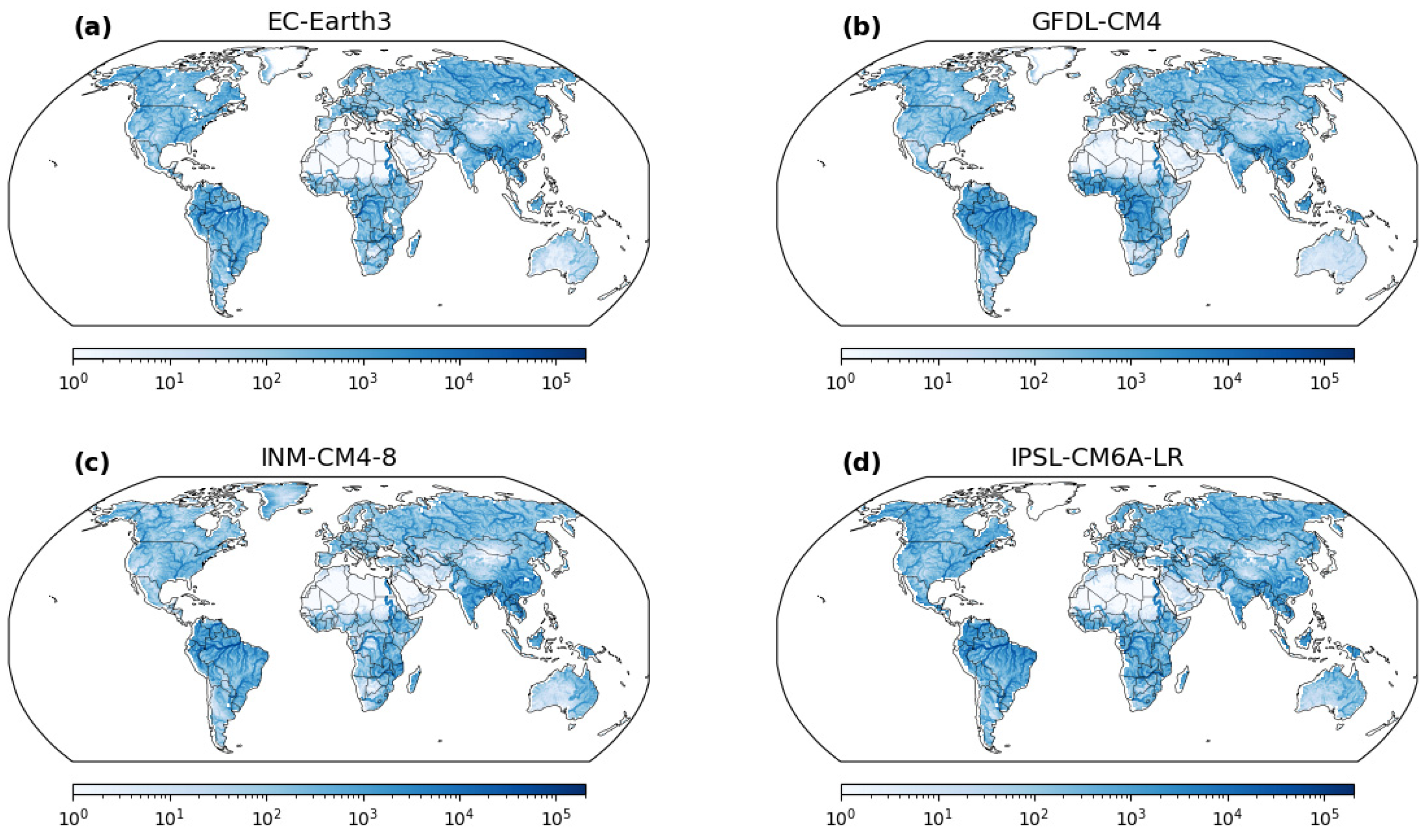
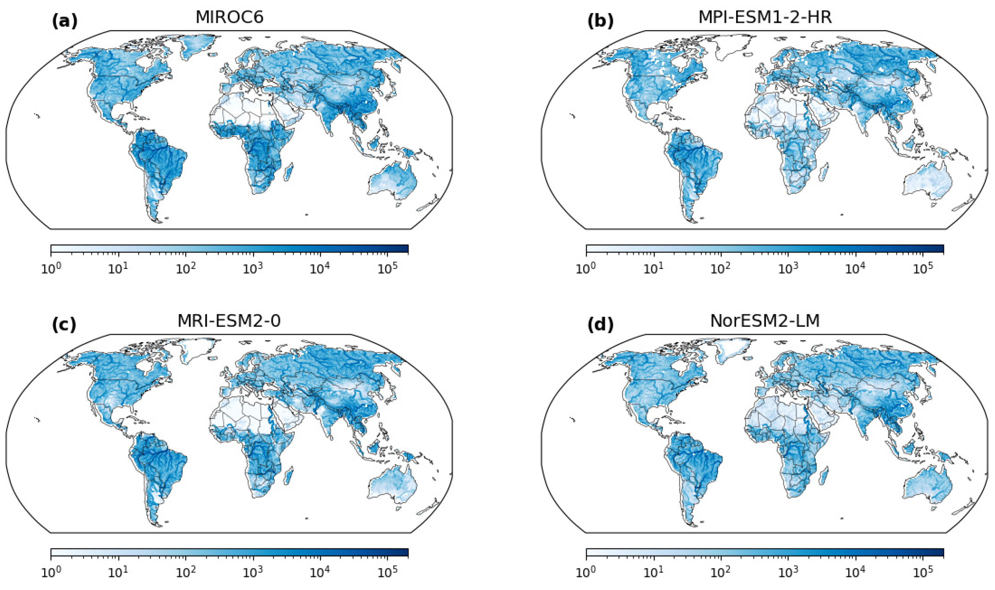
Figure 1 illustrates a grid-based comparison of global mean annual maximum discharge generated by CaMa-Flood with nine GCM-based runoff datasets during 1850–2015. Each panel represents the simulated discharge from a specific GCM-based dataset, and the map reveals significant spatial variability in discharge across different regions. In Figure 1, the map uses darker colors to represent regions with high discharge values, indicating the locations of large rivers in the world. For example, major rivers such as the Amazon in South America, the Nile in Africa, the Yangtze in Asia, and the Mississippi in North America could be visualized as darker regions in the figure due to their substantial annual maximum discharge. Conversely, lighter colors might signify regions with lower discharge values, indicating dry or arid areas. For instance, parts of deserts such as the Sahara in Africa, the Arabian Desert in the Middle East, and the Atacama Desert in South America might appear as lighter shades in the figure, representing the lower annual maximum discharge in these dry regions. The comparison also reveals distinct discharge patterns among the GCMs, with some consistently overestimating and others underestimating discharge magnitudes. These differences stem from varying representations of land surface processes, precipitation patterns, and hydrological parameterizations in the GCMs. Additionally, certain regions display GCM-induced biases, indicating the necessity of identifying and quantifying these discrepancies for accurate hydrological modeling and decision making. The color patterns further highlight the suitability of specific GCMs in capturing hydrological behavior in different regions, with GCMs closely resembling CaMa-Flood’s discharge distribution being more reliable.

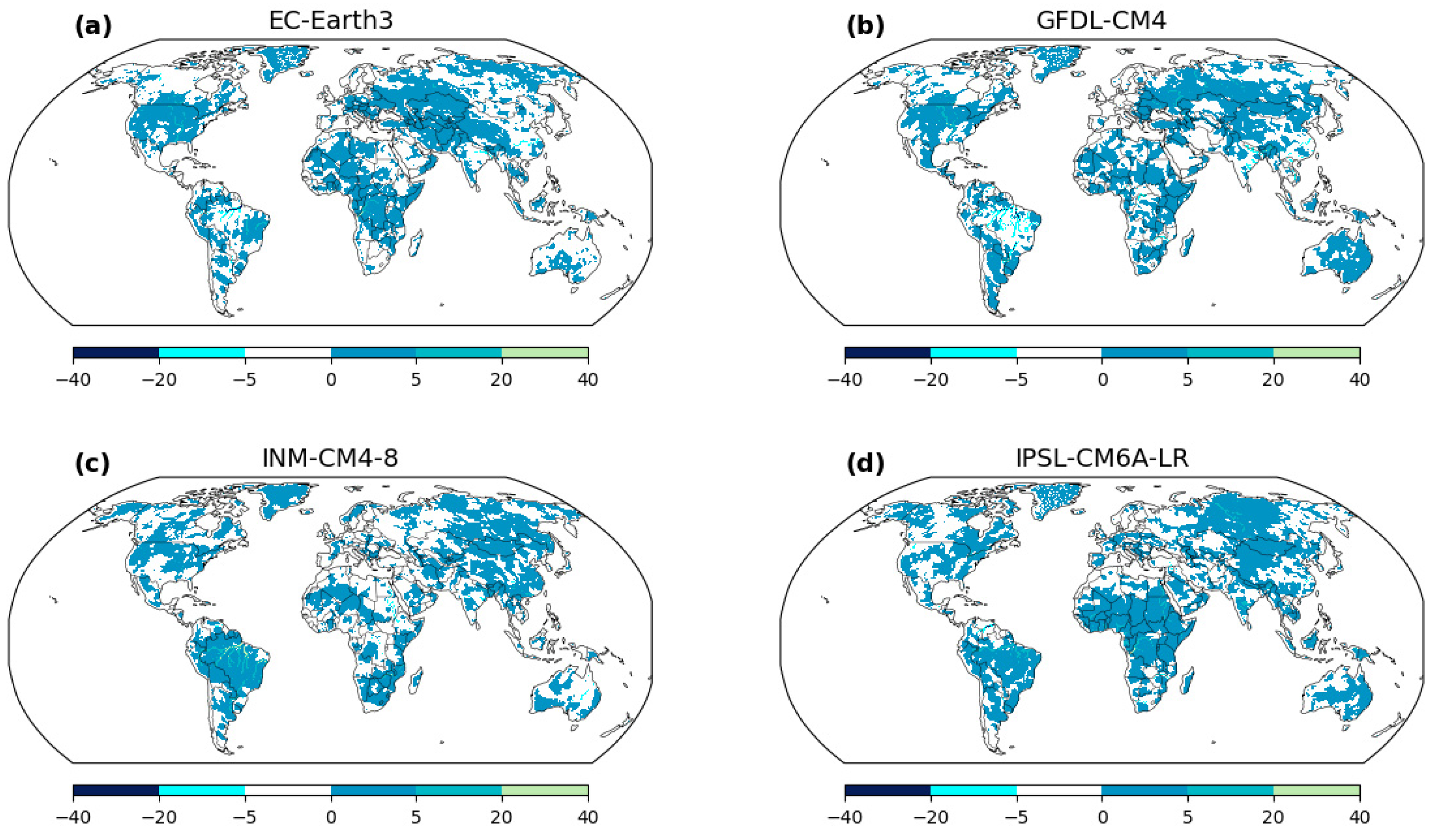
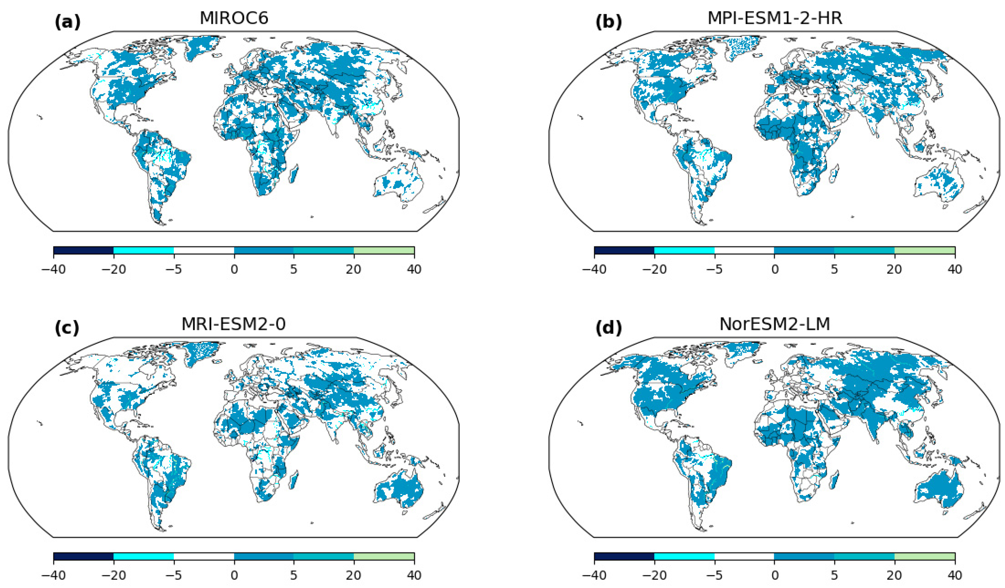
Figure 2 reveals the slope of the annual maximum discharge trends during 1850–2015 for each grid, providing insights into regional differences and disparities among GCMs in capturing hydrological behavior. The color-coded representation shows pronounced regional variability, with some areas displaying positive slopes indicating an increasing trend in annual maximum discharge, while others show negative slopes indicating a decreasing trend. In most parts of the world, the color-coded slopes indicate a positive trend, suggesting an increasing pattern in annual maximum discharge over the study period. This observation aligns with the general understanding of global hydrological changes associated with climate variability and human activities [33]. However, within specific regions, such as the Amazon River basin, negative slopes are evident, indicating a decreasing trend in annual maximum discharge. These localized variations could be linked to the complex interactions of regional climate patterns, land use changes, and hydrological responses. Comparing the panels highlights the influence of different GCMs on the simulated discharge trends. The discrepancies in capturing the hydrological behavior of regions, particularly in areas such as the Amazon River basin can be observed in Figure 2. For some GCMs, the rivers within the Amazon basin show an increasing trend in annual maximum discharge, while other GCMs exhibit a decreasing trend. These differences highlight the sensitivity of hydrological modeling to GCM selection and emphasize the necessity of carefully choosing appropriate GCMs for accurate simulations. Each GCM exhibits varying spatial patterns in the slopes, leading to disparities in the representation of hydrological behavior across regions. Some GCMs may capture specific regional trends more accurately, while others may have biases or uncertainties in their simulations. The distinct color ranges representing different slopes offer a quantified measure of the trend in annual maximum discharge. Lighter colors indicate steeper slopes, representing significant decreases in discharge over time, while darker colors illustrate gentler slopes, indicating relatively stable or slightly increasing discharge trends.

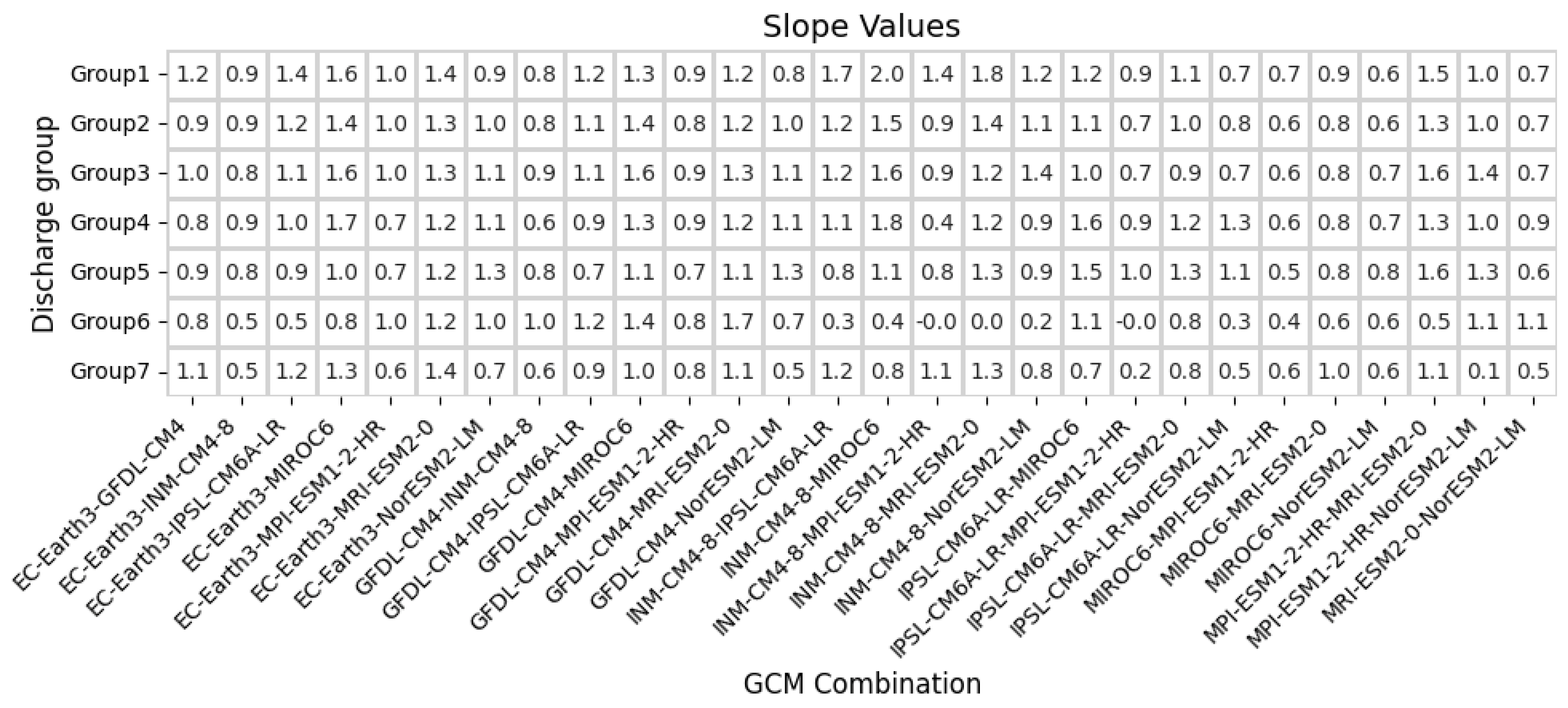
Figure 3 illustrates the slope of the annual maximum discharge across seven discharge groups for two combinations of GCMs. The data reveal crucial insights into the sensitivity of simulated discharge to GCM selection within distinct discharge ranges. Among the two combinations of GCMs, Experiment1 (EC-Earth3 and GFDL-CM4) and Experiment2 (EC-Earth3 and INM-CM4-8), the slopes vary considerably, indicating substantial disparities in the simulated discharge trends. For instance, Experiment1, exhibits a diverse range of slope values for different discharge groups. Notably, in Group1, EC-Earth3 displays a slope of 1.22, while in Group6, the slope decreases to 0.76, showcasing a decreasing trend. Similarly, GFDL-CM4 portrays varying slope values, with a relatively higher slope of 1.66 in Group4 and a lower slope of 0.60 in Group7. Conversely, Experiment2, exhibits a more consistent slope pattern, with relatively minor fluctuations among the discharge groups. In Group1, both EC-Earth3 and INM-CM4-8 depict slopes of 0.93 and 0.75, respectively, indicating a relatively stable trend in this discharge range. Notably, Group6 shows a significant decrease in slope for INM-CM4-8, reaching 0.25, suggesting a pronounced decreasing trend compared to the other groups. These findings highlight the importance of GCM selection in assessing future hydrological changes and emphasize that some discharge groups may be more sensitive to specific GCMs. Furthermore, the observed variability in slope values among discharge groups underscores the complex and nonlinear nature of climate–hydrology relationships, necessitating cautious consideration of GCMs in climate change impact studies for effective water resource management and flood prediction.

3.2. Reference Map for Extreme Flood Estimation Using Stationary and Nonstationary Methods

In this section, we present a comprehensive assessment of grid maps’ suitability for estimating extreme floods using stationary or nonstationary methods. The grid maps serve as a crucial reference, allowing us to determine the most appropriate approach for analyzing extreme flood events in different regions. Through this analysis, we aim to provide valuable insights into the choice of methodologies for accurate and robust extreme flood estimation in various geographic areas.

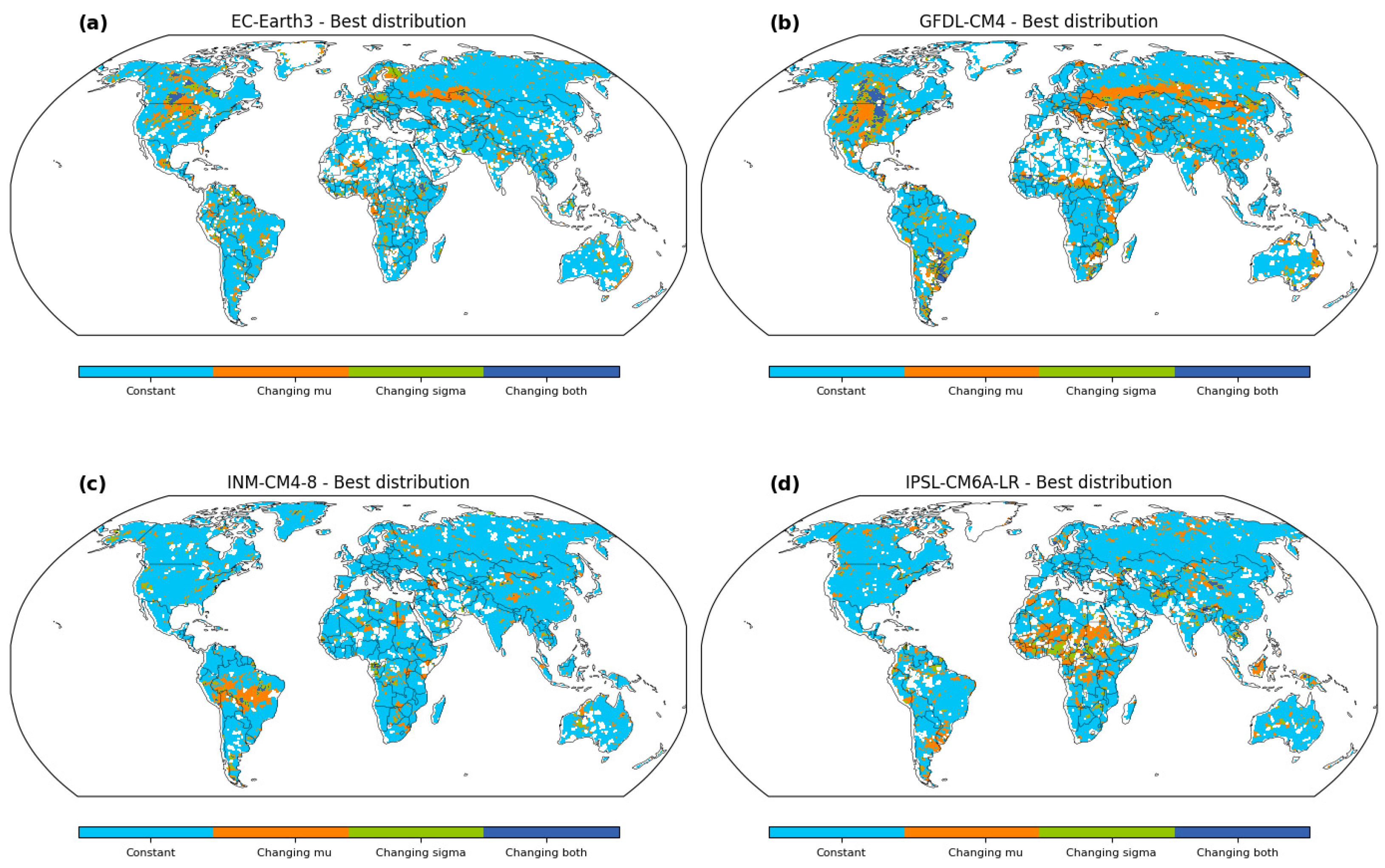
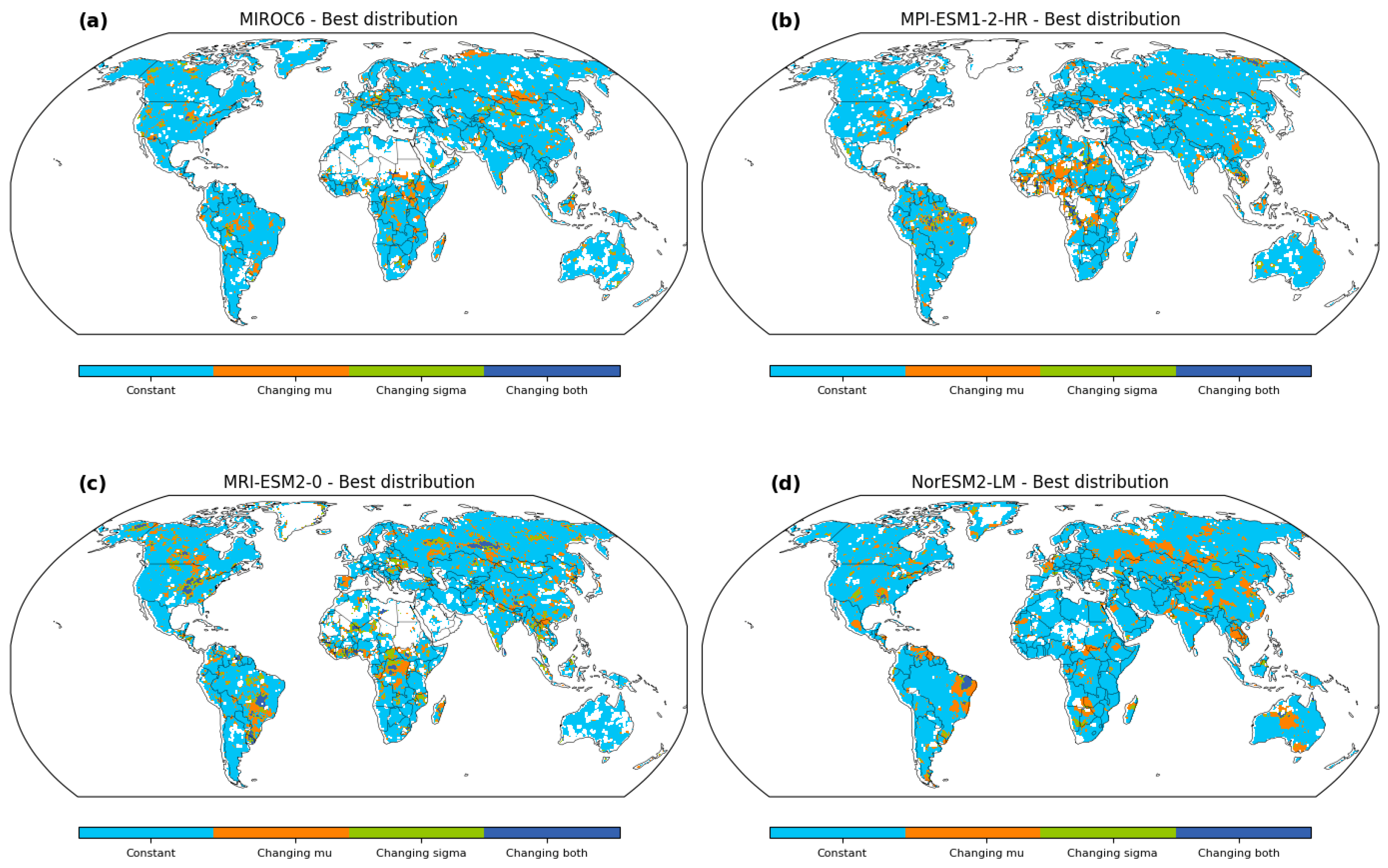
Figure 4 reveals the spatial variation and GCM differences in the best distribution for extreme flood estimation using the CaMa-Flood model with different GCM-output runoff datasets. The results reveal that the majority of the regions exhibit a constant distribution, indicating a stationary method. However, upon closer examination, notable variations are observed in specific areas. For instance, regions such as the United States, the Amazon basin, and parts of northern Asia and Africa exhibit changing mean (changing mu), suggesting the utilization of nonstationary approaches in those locations. This spatial difference highlights the importance of considering nonstationary methods in certain regions to better capture the complexities of extreme flood events. Moreover, the variations among GCMs are also apparent, with some regions favoring changing mean (mu), while others show a preference for changing scale (sigma). Remarkably, the spatial variation is not the only contributing factor to the differences in best distribution. Distinct GCM-output runoff datasets also lead to disparities in the estimated flood frequency. Certain regions are more compatible with changing μ in one GCM, while others exhibit changing σ in another GCM. Notably, in the Amazon River basin, for instance, the ISPL-CM6A-LR GCM suggests that the changing mean (changing μ) approach yields the most accurate results, while other GCMs indicate that the stationary method is more appropriate. On the other hand, for the GFDL-CM4 GCM, regions such as the United States, northern Asia, and Africa exhibit characteristics that favor the nonstationary method as the best fit. In particular, the changing scale (changing σ) approach provides a better estimation for extreme floods in these areas, as indicated by the lowest BIC values. Furthermore, when analyzing the results from the INM-CM4-8 GCM, the regions in India demonstrate a preference for the nonstationary method, suggesting that both changing mean (changing μ) and changing scale (changing σ) covariate functions are necessary for an accurate flood frequency estimation. For a more detailed analysis of geological variations and GCM-specific results, refer to Figure 4 and Figure A4.

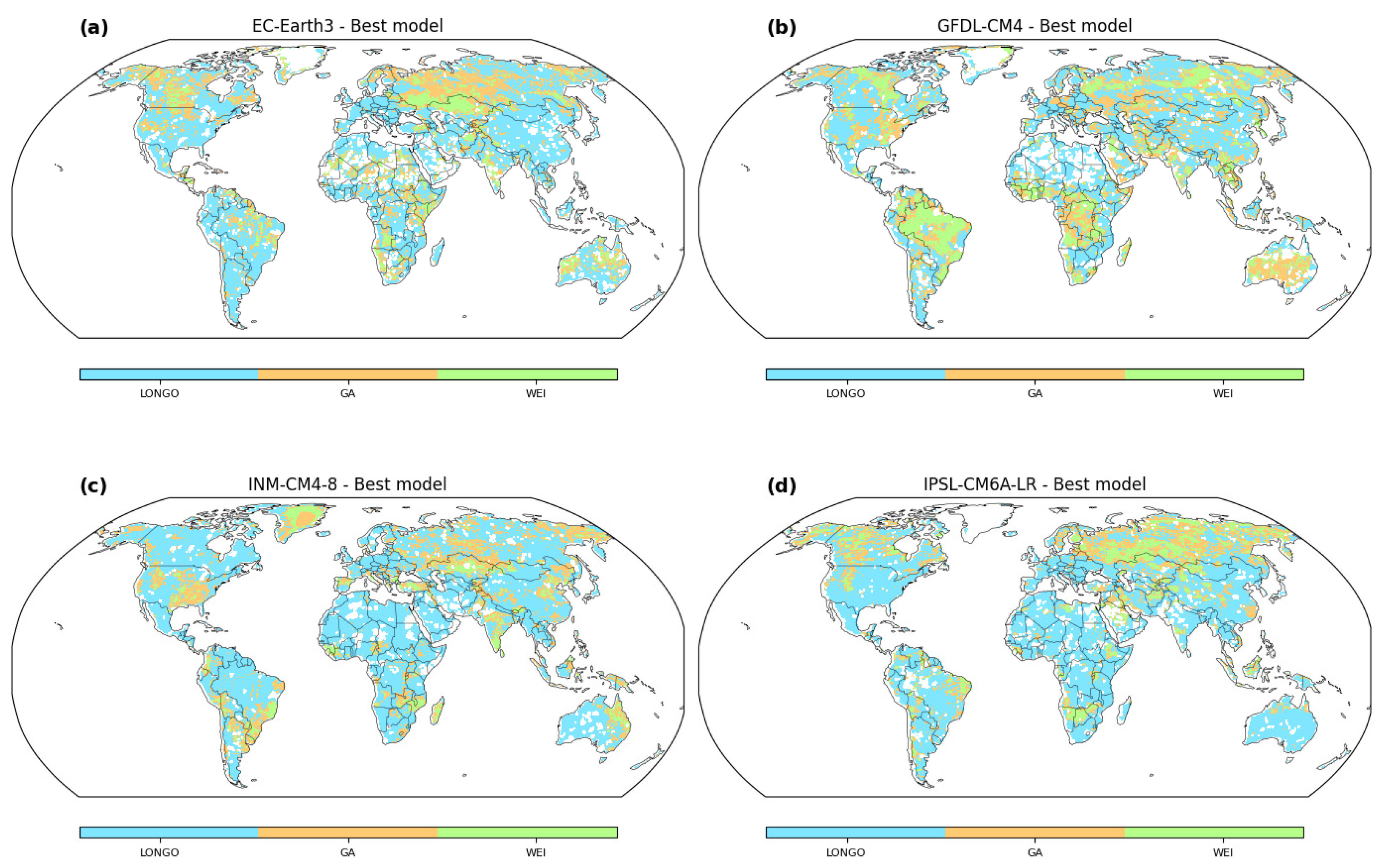
Figure 5 presents a comprehensive assessment of the best distribution models for extreme flood estimation using the CaMa-Flood model in conjunction with various GCM-output runoff datasets. The selection of the optimal model is determined by the Bayesian Information Criterion (BIC), a widely accepted metric that balances model complexity and goodness-of-fit. This figure provides valuable insights into the suitability of different distribution models—specifically, the Lognormal (LONGO), Generalized Extreme Value (GA), and Weibull (WEI) distributions—across diverse geographical regions. The results unveil most regions characterized by a consistent distribution pattern, suggestive of a LONGO model. However, upon closer scrutiny, significant divergences come to light in specific geographic areas. Notably, regions including Australia, the Amazon basin, and portions of northern Asia and North America exhibit distinctive model preferences, indicating the need for employing GA or WEI approaches. This geographical contrast underscores the significance of tailoring methodologies to capture the intricacies of extreme flood events in specific regions. Furthermore, the disparities in model preferences are notably influenced by variations among GCMs. Different regions exhibit a propensity for specific model types, with some favoring a particular model parameterization. Interestingly, the geological characteristics are not the sole driver of these discrepancies. Disparate GCM-output runoff datasets also contribute to variations in estimated flood frequency. Specific regions align more closely with a certain model in one GCM, while in another GCM, a different model may be more suitable. For example, in the Amazon River basin, the ISPL-CM6A-LR GCM suggests that the LONGO yields the most accurate results, while GFDL-CM4 GCM propose the WEI model as more appropriate. Similarly, for the GFDL-CM4 GCM, regions such as the United States, northern Asia, and Africa exhibit characteristics that favor a specific model, specifically the GA and WEI models. Additionally, when assessing outcomes from the EC-Earth3 GCM, regions in European exhibit a preference for the LONGO and WEI models.

Figure 6 presents a pivotal reference map for the estimation of extreme floods, adeptly merging outcomes from all nine GCM runoff products in conjunction with the CaMa-Flood model. This synthesis offers a comprehensive global overview, shedding light on the geographic suitability of stationary and nonstationary methods for extreme flood estimation. The analysis employs the Generalized Additive Models for Location, Scale, and Shape (GAMLSS) methodology, encompassing three distinct models characterized by four parameter types: changing mean (μ), changing scale (σ), a combination of both (nonstationary), and the stationary method with constant parameters. This approach provides a robust framework for discerning the dominant methodological choice across diverse geographical regions. Notably, this reference map underscores the dynamic interplay between geological attributes and the appropriateness of different flood estimation approaches. As demonstrated by the results, a clear pattern emerges, revealing regions where the stationary method is well-suited and areas where nonstationary methods offer enhanced accuracy. To illustrate, consider the Amazon basin. Here, the intricate hydrological dynamics necessitate a nonstationary approach, specifically employing the changing mean (μ) models, as evidenced by the merger of GCM-specific outcomes. In contrast, most regions characterized by relatively stable hydrological regimes, exhibit a strong propensity for the stationary method, underlining the importance of tailoring methodologies to the distinct characteristics of each geographic area. Of particular interest, the nonstationary method is spatially dispersed across the globe and of limited size. The proportional representation of nonstationary and stationary methods on this map underscores the selective prevalence of these methodologies, demonstrating a proportion of approximately 1:23. While the stationary method dominates most regions, critical clusters necessitate the nonstationary framework for accurate flood estimation. This nuanced depiction guides the selection of methodologies, contributing to more effective flood risk assessments and management strategies. The reference map provides a quantitative depiction of this dichotomy, allowing us to discern the proportional distribution of stationary and nonstationary methods across the globe.

3.3. Application of Referenced Map for Estimating Flood Magnitudes Using Stationary and Nonstationary Methods

In this section, we delve into the practical implications of the referenced map, obtained through a meticulous evaluation of grid suitability for stationary and nonstationary methods using the Bayesian Information Criterion (BIC) analysis. We begin by showcasing the application of these methods in estimating global 100-year flood magnitudes and subsequently provide compelling examples that vividly illustrate the disparities between the two approaches.

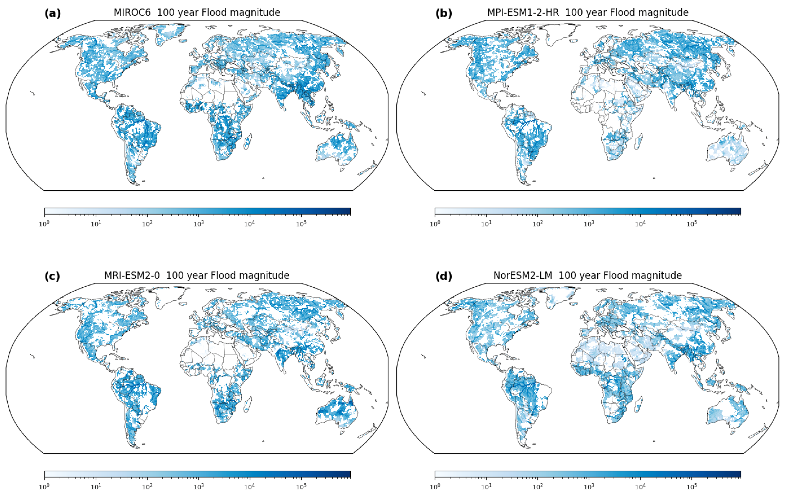
Figure 7 vividly portrays the global distribution of estimated 100-year flood magnitudes utilizing the stationary method. This depiction emerges from the utilization of the CaMa-Flood model, driven by diverse GCM-output runoff datasets. The figure serves as a visual guide to the spatial variability of flood magnitudes across the globe. The amalgamation of these datasets culminates in a comprehensive assessment of flood magnitudes, unraveling the intricate interplay between climatic nuances and hydrological responses. The variegated palette of colors across the map signifies distinct hydrological regimes, reflecting the multifaceted nature of flood dynamics. Of paramount significance is the discernible spatial heterogeneity in estimated flood magnitudes. The color gradations on the map reflect variations in flood magnitudes. Darker shades correspond to regions with higher discharge values, highlighting areas with significant annual maximum discharge such as major rivers such as the Amazon, Nile, Yangtze, and Mississippi. In contrast, lighter shades indicate lower discharge values, often associated with arid or drier regions. Regions exhibiting profound color transitions indicate zones of heightened hydrological activity, underscoring their vulnerability to extreme flood events. This visual narrative reinforces the pivotal role of nonstationary methods, as climatic fluctuations and hydrological shifts accentuate the limitations of stationary approaches in accurately predicting and preparing for such events. The map also underscores divergent discharge patterns arising from the utilization of different GCMs, showcasing the variability introduced by distinct representations of land surface processes, precipitation patterns, and hydrological parameterizations.

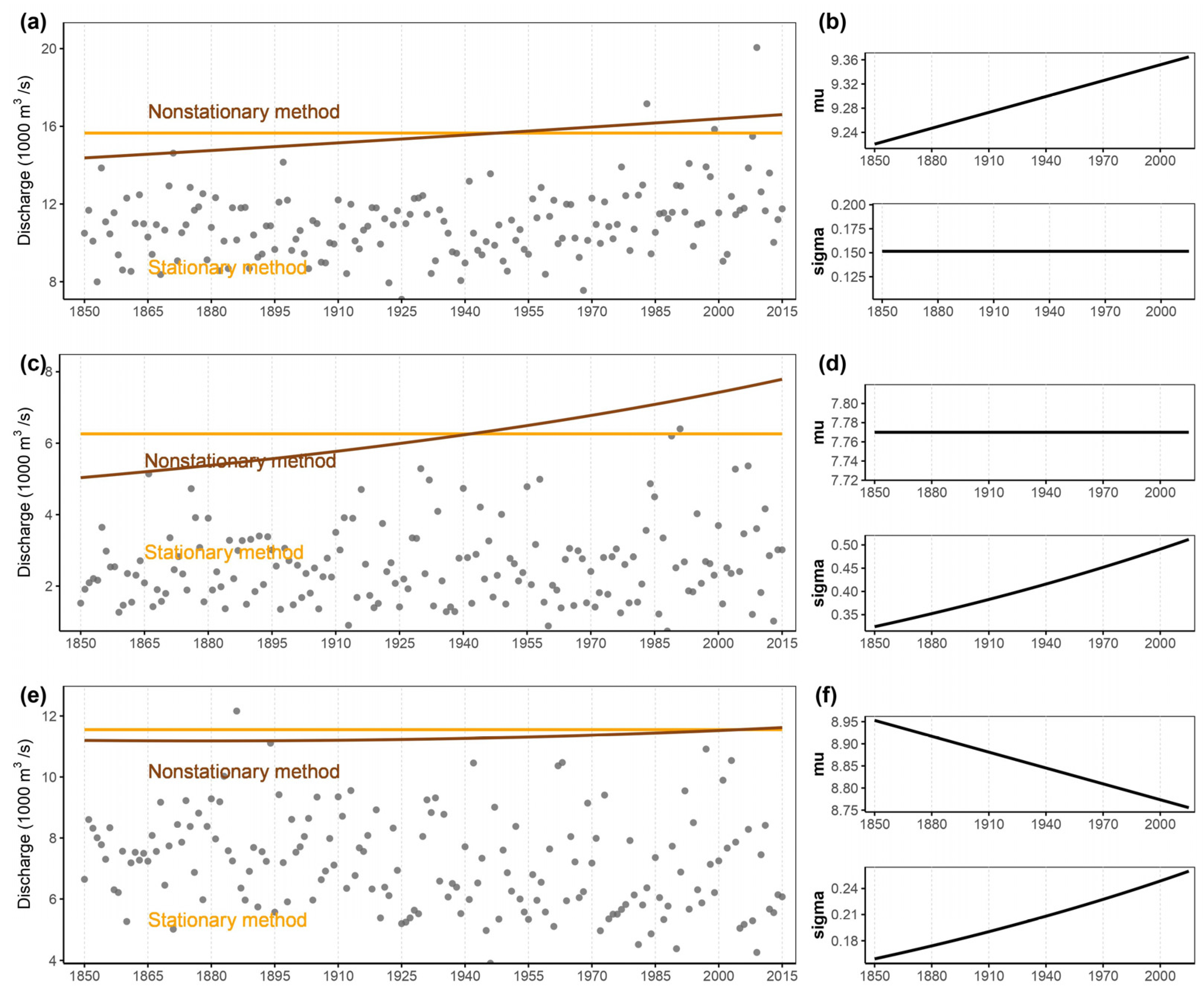
Figure 8 serves as a focal point in our investigation, spotlighting the crucial disparities between stationary and nonstationary methods. It exemplifies selected representative grids from the reference map, each identified as necessitating nonstationary methodologies due to specific hydrological nuances. The nonstationary method, encompassing three pivotal scenarios—changing μ, altering σ, and simultaneous variations in both—delineates the intricate interplay of hydrological parameters. The significance of nonstationary methods becomes evident as we analyze the changing patterns of flood magnitudes over time. When μ is subjected to variations, it leads to discernible shifts in the central tendency of flood magnitudes, reflecting alterations in hydrological behavior. The alteration of σ, conversely, translates to shifts in the variability of flood magnitudes, indicative of changing flood patterns. Notably, when both μ and σ are simultaneously altered, it highlights the intricate interplay between multiple hydrological factors. In contrast, the stationary method presents a static perspective of flood magnitudes, failing to capture the temporal evolution inherent to hydrological systems. This simplified approach overlooks the nuanced interplay between climatic shifts and hydrological responses. The referenced map informs our estimation of flood magnitudes, guiding us towards an understanding of the spatial variability. Figure 8 accentuates the necessity of accommodating nonstationarity, offering a sobering reminder of the importance of adaptive methodologies for accurate flood risk assessment and management.

4. Discussion

4.1. GCMs Unveiling Spatial Suitability: Reference Map for Methodological Selection

Our study introduces a pioneering approach to enhance flood risk assessment by constructing a reference map that delineates the spatial suitability of stationary and nonstationary methods. This map, as depicted in Figure 6, encapsulates a wealth of information critical to flood estimation, making it an invaluable tool for policymakers, hydrologists, and decision makers. The delineation of regions where stationary methods prevail and areas where nonstationary approaches are imperative lays the foundation for a more refined and contextually appropriate flood analysis. The map’s spatial patterns are deeply rooted in the intricate interplay between geological characteristics, hydrological dynamics, and climatic variability. The regions favoring nonstationary methods, exemplified by changing mean (μ) or changing scale (σ) scenarios, underscore the underlying shifts in hydrological behavior [33]. In contrast, the prevalence of stationary methods in more stable hydrological regimes reflects their adequacy for capturing long-term trends. This nuanced approach recognizes the inherent complexity of hydrological systems and provides a comprehensive basis for methodological selection.

The map provides valuable insights into the spatial distribution of suitable flood frequency analysis methodologies across the study area. Most regions are characterized by the constant distribution, representing the stationary method, where both the mean (μ) and scale (σ) parameters remain constant over time and space. This consistency indicates areas where the flood magnitudes exhibit relatively stable behavior, unaffected by significant temporal or spatial variations. In contrast, certain locations stand out with the changing μ distribution, which implies that the mean flood magnitude exhibits temporal variations. These regions experience dynamic hydrological conditions, and the flood events’ mean intensity varies over different time periods. These areas demand nonstationary approaches to account for these temporal fluctuations and obtain accurate flood estimations. Similarly, other areas exhibit the changing σ distribution, indicating spatial variations in flood variability while maintaining a constant mean flood magnitude. These regions may face altered flood characteristics due to factors such as land use changes, urbanization, or climate-induced alterations in precipitation patterns. Such changes in flood variability necessitate the application of nonstationary methods for precise flood estimations. Distinct GCM-output runoff datasets also lead to disparities in the estimated flood frequency. Certain regions are more compatible with changing μ in one GCM, while others exhibit changing σ in another GCM. This highlights the significance of understanding the nuances introduced by each GCM and its impact on flood frequency analysis. The identification of geological differences and GCM disparities in the best distribution is crucial for tailored flood risk management strategies. By accounting for spatial variations and considering the influence of different GCMs, decision makers and researchers can adopt suitable modeling approaches for each region, leading to more accurate estimations and improved flood risk preparedness.

4.2. Implications of Nonstationarity on Extreme Flood Estimation

The implications of our study transcend theoretical musings, manifesting tangibly in the realm of practical flood risk management [34,35,36]. Figure 8 illuminates the stark divergence between stationary and nonstationary approaches, serving as a visual allegory for the consequential differences in extreme flood estimation. The scenarios of changing mean (μ) and changing scale (σ) underscore the intrinsic dynamism within hydrological systems, where flood magnitudes are not static entities but evolve over time. This realization underscores a paradigm shift in our understanding of extreme events, emphasizing the role of nonstationary methodologies as torchbearers of accurate estimation. A poignant message emanates from Figure 8—the potential underestimation of extreme flood magnitudes by stationary methods. The inherent assumption of stationarity, rooted in historical data and temporal constancy, falls short in capturing the inherent variability introduced by changing climatic conditions. Such underestimations have profound implications for risk assessment and preparedness. The consequences of underestimating extreme flood magnitudes could be dire, resulting in inadequately designed infrastructure, ineffective floodplain management, and compromised disaster response strategies. Nonstationary methodologies emerge as the guiding light, providing a nuanced and comprehensive lens through which extreme flood events can be understood. By accounting for temporal and spatial variability, these approaches offer a realistic portrayal of the evolving hydrological landscape. This resonates deeply in the realm of policy formulation, where accurate estimations underpin effective decision making. Resilient infrastructure, adaptive land use planning, and robust emergency response mechanisms can only be realized by embracing the dynamic nature of hydrological systems—a realization underscored by the implications of nonstationary methodologies.

4.3. Navigating Uncertainty: GCMs and Model Selection

Our exploration of GCMs introduces a layer of uncertainty into the tapestry of flood estimation. The intricate interplay between GCMs and distribution models, highlighted by the disparities in model preferences across regions (Figure 5), is a microcosm of the challenges inherent in climate and hydrological research. This uncertainty magnifies the importance of meticulous GCM evaluation, calibration, and validation. Accurate flood predictions hinge upon a nuanced understanding of the strengths and limitations of each GCM, illuminating a path towards robust modeling practices. The fusion of GCM characteristics with distribution model selection elucidates the multifaceted nature of climate–hydrology interactions. It beckons us to acknowledge the complexity of the climate system and its cascading influence on hydrological behavior. The impact transcends the realm of flood estimation, permeating diverse disciplines that rely on accurate climate projections. From agricultural planning to urban design, from water resource management to biodiversity conservation, the fidelity of climate models reverberates across societal and ecological domains. In navigating this sea of uncertainty, the onus lies upon researchers and stakeholders to collaboratively unravel the intricacies of GCMs. Rigorous scrutiny, ensemble modeling, and validation against real-world observations can chip away at the veil of uncertainty, enhancing the reliability of flood predictions. Beyond the immediate scope of hydrological research, this endeavor underscores the interconnectedness of disciplines under the umbrella of climate science.

4.4. Limitation and Future Research

While our research marks a significant step in improving flood risk assessment by introducing a reference map for methodological selection, several limitations warrant consideration. The use of Generalized Additive Models for Location, Scale, and Shape (GAMLSS) presents certain constraints, and future investigations could explore alternative statistical methods or hybrids for enhanced model selection. Additionally, the reference map’s resolution may not capture localized variations in hydrological behavior, suggesting a need for higher-resolution mapping. The choice of a 0.25-degree spatial resolution in our reference map was influenced by the availability of Global Climate Model (GCM) outputs. While this resolution serves the purpose of large-domain flood-related decision making, it is important to acknowledge that it may result in some underestimation of peak flow at smaller scales. Future research endeavors could explore the feasibility of employing higher resolutions, such as 0.01 degrees, for more localized studies, which could provide a more fine-grained representation of hydrological conditions. Looking ahead, the reference map offers a versatile platform for various lines of inquiry. Researchers can leverage this map to estimate extreme flood characteristics, encompassing flood magnitudes and inundation extents. Validation, a critical step, involves comparing model-derived estimates with historical flood events, field observations, or remote sensing data to ensure the reliability of our methodology. Furthermore, future research can delve into exploring the disparities between nonstationary and stationary methods for estimating extreme floods. This investigation can shed light on the contrasting performance of these methodologies and the implications for flood risk assessment. Additionally, there is ample scope for conducting flood analyses under climate change scenarios, utilizing the reference map as a foundation for understanding how evolving climatic conditions may impact future flood events. In summary, while the 0.25-degree spatial resolution was chosen due to GCM data constraints and the requirements of large-scale flood-related decision making, the potential exists for future research to employ higher resolutions for localized investigations. The reference map serves as a valuable resource for estimating and validating extreme flood events, exploring methodological disparities, and considering the influence of climate change on future flood scenarios.

5. Conclusions

Our study makes significant strides in advancing flood risk assessment by introducing a reference map that guides the selection of suitable methodologies for extreme flood estimation. The map encapsulates the spatial intricacies of hydrological behavior, unveiling the spatial divide between stationary and nonstationary methods. This novel approach, rooted in robust hydrological modeling and GCM data, provides a comprehensive framework for accurately estimating extreme flood events. As climate change intensifies, the need for adaptive and contextually tailored methodologies becomes ever more apparent. Our findings emphasize the inadequacy of static approaches and illuminate the potential of nonstationary methods to provide a more comprehensive understanding of evolving hydrological dynamics. The implications for flood risk management are profound, with direct relevance to infrastructure design, policy formulation, and disaster preparedness. In conclusion, our study bridges the gap between climatic variability, hydrological dynamics, and flood estimation methodologies. The reference map serves as a powerful tool to guide methodological selection, harnessing the intricate nuances of hydrological behavior to enhance the accuracy and reliability of extreme flood estimation. As we navigate an era of heightened climate uncertainty, the integration of adaptive methodologies and robust modeling practices remains paramount for effective flood risk assessment and management.

References

1. Slater, L.J.; Anderson, B.; Buechel, M.; Dadson, S.; Han, S.; Harrigan, S.; Kelder, T.; Kowal, K.; Lees, T.; Matthews, T.; et al. Nonstationary weather and water extremes: A review of methods for their detection, attribution, and management. Hydrol. Earth Syst. Sci. Discuss. 2021, 25, 3897–3935. [Google Scholar] [CrossRef]
2. UNDRR. Economic Losses, Poverty & Disasters: 1998–2017. 2018. Available online: https://www.undrr.org/publication/economic-losses-poverty-disasters-1998-2017 (accessed on 4 August 2023).
3. Bouchard, J.P.; Pretorius, T.B.; Kramers-Olen, A.L.; Padmanabhanunni, A.; Stiegler, N. Global warming and psychotraumatology of natural disasters: The case of the deadly rains and floods of April 2022 in South Africa. Ann. Médico-Psychol. Rev. Psychiatr. 2023, 181, 234–239. [Google Scholar] [CrossRef]
4. Hirabayashi, Y.; Mahendran, R.; Koirala, S.; Konoshima, L.; Yamazaki, D.; Watanabe, S.; Kim, H.; Kanae, S. Global flood risk under climate change. Nat. Clim. Chang. 2013, 3, 816–821. [Google Scholar] [CrossRef]
5. Hoegh-Guldberg, O.; Jacob, D.; Taylor, M.; Bindi, M.; Brown, S.; Camilloni, I. Impacts of 1.5 °C of global warming on natural and human systems. In Global Warming of 1.5 °C; An IPCC Special Report; IPCC: Geneva, Switzerland, 2018. [Google Scholar]
6. Blum, A.G.; Ferraro, P.J.; Archfield, S.A.; Ryberg, K.R. Causal Effect of Impervious Cover on Annual Flood Magnitude for the United States. Geophys. Res. Lett. 2020, 47, e2019GL086480. [Google Scholar] [CrossRef]
7. Vogel, R.M.; Yaindl, C.; Walter, M. Nonstationarity: Flood Magnification and Recurrence Reduction Factors in the United States1. JAWRA J. Am. Water Resour. Assoc. 2011, 47, 464–474. [Google Scholar] [CrossRef]
8. Yan, L.; Xiong, L.; Ruan, G.; Zhang, M.; Xu, C.-Y. Design flood estimation with varying record lengths in Norway under stationarity and nonstationarity scenarios. Hydrol. Res. 2021, 52, 1596–1614. [Google Scholar] [CrossRef]
9. Yan, L.; Xiong, L.; Guo, S.; Xu, C.-Y.; Xia, J.; Du, T. Comparison of four nonstationary hydrologic design methods for changing environment. J. Hydrol. 2017, 551, 132–150. [Google Scholar] [CrossRef]
10. Salas, J.D.; Obeysekera, J.; Vogel, R.M. Techniques for assessing water infrastructure for nonstationary extreme events: A review. Hydrol. Sci. J. 2018, 63, 325–352. [Google Scholar] [CrossRef]
11. Berghuijs, W.R.; Aalbers, E.E.; Larsen, J.R.; Trancoso, R.; Woods, R.A. Recent changes in extreme floods across multiple continents. Environ. Res. Lett. 2017, 12, 114035. [Google Scholar] [CrossRef]
12. Archfield, S.A.; Hirsch, R.M.; Viglione, A.; Blöschl, G. Fragmented patterns of flood change across the United States. Geophys. Res. Lett. 2016, 43, 10232–10239. [Google Scholar] [CrossRef]
13. Eastoe, E.F. Nonstationarity in peaks-over-threshold river flows: A regional random effects model. Environmetrics 2019, 30, e2560. [Google Scholar] [CrossRef]
14. Hecht, J.S.; Vogel, R.M. Updating urban design floods for changes in central tendency and variability using regression. Adv. Water Resour. 2020, 136, 103484. [Google Scholar] [CrossRef]
15. Steirou, E.; Gerlitz, L.; Apel, H.; Sun, X.; Merz, B. Climate influences on flood probabilities across Europe. Hydrol. Earth Syst. Sci. 2019, 23, 1305–1322. [Google Scholar] [CrossRef]
16. Prosdocimi, I.; Kjeldsen, T.R.; Miller, J.D. Detection and attribution of urbanization effect on flood extremes using nonstationary flood-frequency models. Water Resour. Res. 2015, 51, 4244–4262. [Google Scholar] [CrossRef]
17. Slater, L.; Villarini, G.; Archfield, S.; Faulkner, D.; Lamb, R.; Khouakhi, A.; Yin, J. Global changes in 20-year, 50-year, and 100-year river floods. Geophys. Res. Lett. 2021, 48, e2020GL091824. [Google Scholar] [CrossRef]
18. Rigby, R.; Stasinopoulos, M.; Heller, G.; De Bastiani, F. Distributions for Modelling Location, Scale and Shape: Using GAMLSS in R; CRC Press: Boca Raton, FL, USA, 2019. [Google Scholar]
19. Villarini, G.; Smith, J.A.; Serinaldi, F.; Bales, J.; Bates, P.D.; Krajewski, W.F. Flood frequency analysis for nonstationary annual peak records in an urban drainage basin. Adv. Water Resour. 2009, 32, 1255–1266. [Google Scholar] [CrossRef]
20. López, J.; Francés, F. Non-stationary flood frequency analysis in continental Spanish rivers, using climate and reservoir indices as external covariates. Hydrol. Earth Syst. Sci. 2013, 17, 3189–3203. [Google Scholar] [CrossRef]
21. Faulkner, D.; Warren, S.; Spencer, P.; Sharkey, P. Can we still predict the future from the past? Implementing non-stationary flood frequency analysis in the UK. J. Flood Risk Manag. 2020, 13, e12582. [Google Scholar] [CrossRef]
22. Towe, R.; Tawn, J.; Eastoe, E.; Lamb, R. Modelling the Clustering of Extreme Events for Short-Term Risk Assessment. J. Agric. Biol. Environ. Stat. 2020, 25, 32–53. [Google Scholar] [CrossRef]
23. Zhang, T.; Wang, Y.; Wang, B.; Tan, S.; Feng, P. Nonstationary Flood Frequency Analysis Using Univariate and Bivariate Time-Varying Models Based on GAMLSS. Water 2018, 10, 819. [Google Scholar] [CrossRef]
24. Rigby, R.A.; Stasinopoulos, M.D. Mean and Dispersion Additive Models. In Statistical Theory and Computational Aspects of Smoothing; Physica-Verlag HD: Heidelberg, Germany, 1996; pp. 215–230. [Google Scholar]
25. Villarini, G.; Strong, A. Roles of climate and agricultural practices in discharge changes in an agricultural watershed in Iowa. Agric. Ecosyst. Environ. 2014, 188, 204–211. [Google Scholar] [CrossRef]
26. Giuntoli, I.; Villarini, G.; Prudhomme, C.; Hannah, D.M. Uncertainties in projected runoff over the conterminous United States. Clim. Chang. 2018, 150, 149–162. [Google Scholar] [CrossRef]
27. Yamazaki, D.; Kanae, S.; Kim, H.; Oki, T. A physically based description of floodplain inundation dynamics in a global river routing model. Water Resour. Res. 2011, 47, W04501. [Google Scholar] [CrossRef]
28. Kimura, Y.; Hirabayashi, Y.; Kita, Y.; Zhou, X.; Yamazaki, D. Methodology for constructing a flood-hazard map for a future climate. Hydrol. Earth Syst. Sci. 2023, 27, 1627–1644. [Google Scholar] [CrossRef]
29. Markovic, R.D. Probability Functions of the Best Fit to Distributions of Annual Precipitation and Runoff Hydrology. Doctoral Dissertation, Colorado State University, Fort Collins, CO, USA, 1965. [Google Scholar]
30. Vogel, R.M.; Wilson, I. Probability Distribution of Annual Maximum, Mean, and Minimum Streamflows in the United States. J. Hydrol. Eng. 1996, 1, 69–76. [Google Scholar] [CrossRef]
31. Stasinopoulos, M.; Rigby, B.; Akantziliotou, C. Instructions on How to Use the Gamlss Package in R Second Edition. 2008. Available online: https://www.researchgate.net/publication/228429663_Instructions_on_how_to_use_the_gamlss_package_in_R_Second_Edition (accessed on 4 August 2023).
32. Akaike, H. A new look at the statistical model identification. IEEE Trans. Autom. Control 1974, 19, 716–723. [Google Scholar] [CrossRef]
33. Nelson, D.B. Stationarity and persistence in the GARCH (1, 1) model. Econom. Theory 1990, 6, 318–334. [Google Scholar] [CrossRef]
34. Shumway, R.; Stoffer, D. Time Series Analysis and Its Applications with R Examples; Springer: New York, NY, USA, 2011; Volume 9. [Google Scholar]
35. Chen, H.-L.; Rao, A.R. Testing hydrologic time series for stationarity. J. Hydrol. Eng. 2002, 7, 129–136. [Google Scholar] [CrossRef]
36. Buuren, S.v.; Fredriks, M. Worm plot: A simple diagnostic device for modelling growth reference curves. Stat. Med. 2001, 20, 1259–1277. [Google Scholar] [CrossRef]
Figure 1. Mean annual maximum discharge during 1850–2015 using CaMa-Flood model driven by eight GCM-output runoff products. For the remaining results, please see the Figure A1.
Water 15 03835 g001
Figure 2. Slope of the annual maximum discharge during 1850–2015 using CaMa-Flood model driven by eight GCM-output runoff products. For the remaining results, please see the Figure A2.
Water 15 03835 g002
Figure 3. Slope of the annual maximum discharge in seven discharge groups among two combinations of GCMs. The discharge data are categorized into seven groups, representing the ranges [0, 1000, 5000, 10,000, 20,000, 30,000, 40,000, 80,000] m3/s. Each combination of GCMs is used to fit curves among their respective simulations, and the slope of the simulated discharge is calculated within each discharge group.
Water 15 03835 g003
Figure 4. Spatial Variation and GCM Differences in Best Distribution for Extreme Flood Estimation. Constant means the stationary method, while changing mu, changing sigma, and changing both are the nonstationary approaches. For the remaining results, please see the Figure A3.
Water 15 03835 g004
Figure 5. Best distribution model for extreme flood estimation using CaMa-Flood with different GCM-output runoff datasets. The best model is selected in terms of BIC. For the remaining results, please see the Figure A4.
Water 15 03835 g005
Figure 6. Reference map for extreme flood estimation using stationary and nonstationary methods after merging results from all GCMs.
Water 15 03835 g006
Figure 7. One hundred-year flood magnitudes (m3/s) estimated by stationary method based on the annual maximum discharge simulated by CaMa-Flood with different GCM-output runoff datasets.
Water 15 03835 g007
Figure 8. Examples to illustrate the difference of 100-year flood magnitudes (m3/s) estimated by stationary and nonstationary methods (a,c,e). Note that nonstationary conditions have three cases: changing mu, changing sigma, and changing both. We selected three representative grids from the reference map, each identified as necessitating nonstationary methodologies, encompassing three pivotal scenarios—changing μ (b), altering σ (d), and simultaneous variations in both (f).
Water 15 03835 g008