Abstract
The ecological environment in southwestern China is fragile. Due to the significant preferential flow in vertical and horizontal directions and poor water conservation ability, vegetation degradation still exists under conditions of abundant rainfall. Therefore, the pore connectivity and infiltration characteristics in shallow soil under typical local vegetation need to be studied. A calculation model for the vertical connectivity of soil macropores was independently constructed, and differences in soil macropore structures and the degree of vertical connectivity in typical vegetation types (natural secondary forest, natural grassland, Yunnan pine plantation, eucalyptus plantation, cypress plantation, mulberry bushes) were investigated by CT scanning technology of undisturbed soil columns. The results showed that the vertical connectivity of large pores in the shallow soil of the region can be quantitatively described by X-ray tomography, and the total surface area and cumulative curvature of macropores in natural grassland soil were two or three times that in artificial vegetation. The concentration area of macropores in the soil of artificial forestland was closer to the surface, and the tendency of macropore preferred path decreased by 76.18% around 30 cm depth in the soil. The vertical connection of soil macropores in artificial forests was significantly lower than that of natural secondary forestlands (33.03%) and natural grasslands (36.75%). The restoration of the plantation improved surface soil pore structure, and the vertical connectivity of soil is nearly 20% less than that of natural vegetation types (natural secondary forestland, natural grassland), which reduced water outflow rate by nearly 44% and electrolyte content by nearly 14% at a depth of 30 cm. This study provided data and research directions for the study of hydrological processes in local forest vegetation and technical support for solving the problems of soil water loss and forestland water conservation in southwestern China.
1. Introduction
The ecological environment in the southwestern region of China is fragile [1]. Local soil erosion, land desertification, rocky desertification, grassland degradation, and natural disasters occur frequently [2], which seriously restricts economic development [3]. Therefore, in order to alleviate the pressure on the local ecosystem and human economy [4], China has carried out vegetation restoration projects for over 50 years, and vegetation restoration and allocation technologies have made phased progress [5]. However, due to the frequent rainfall and rapid response in hydrological processes, the pore networks in shallow soil hinder water conservation [6], and the deep soil and rock structure accelerate the leakage of water resources, resulting in vegetation degradation in the area.
Water movement of surface soil is the key factor connecting air and deep soil. Soil macropores serve as channels for air, water, nutrient and pollutant retention and transport in soil. Karsanina et al. (2015) found that adjacent macropores connected in different ways can affect the water loss and retention capacity of shallow soil [7]. The spatial structure characteristics of soil macropores, such as length, diameter, volume, and surface area, affect the storage and loss of water and salt [8,9] and are crucial for important ecological restoration issues such as water resource spatial allocation [10,11], the soil erosion process [12], and the migration of nutrients and agricultural and forestry waste pollutants [13,14]. Therefore, studying the influence of the degree of development, spatial structure and connectivity characteristics of macropores in soil on the spatial movement of soil water [15] is extremely important and plays an important role in the development of preferential flow [16] and water conservation in soil [17], the ability of soil macropores to transport surface water is an important parameter that indirectly affects the effectiveness of vegetation restoration [18]. However, the characteristics of soil macropores and their relationship with water transport are some of the difficulties and cutting-edge issues in soil water movement [19], and research quantitatively describing the contribution of soil pore structure to water transport is minor and cannot provide guidance for related production. Therefore, this study considers the quantitative study of soil pore structure based on undisturbed soil and its correlation with water transport to clarify how vegetation cover types affect the connectivity of soil pore networks and their permeability under different soil macropore connectivity conditions.
Currently, many studies on soil macropore water transport use soil profile staining methods; however, the method of simulating soil pore structure by soil profile dyeing results has a great subjective impact [20], and the profile excavation has caused irreversible damage to soil structure. Therefore, this study used a non-invasive imaging technology called X-ray tomography to quantitatively study soil pore structure characteristics [21].
X-ray tomography technology entails placing the undisturbed soil in the CT scanning instrument to obtain the spatial structure information of substances with different densities in the soil and then is used to calculate the spatial distribution structure and quantity of soil pores. This method can provide a complete test sample for the simulation of soil water infiltration under the same soil structure and reduce the influence of soil heterogeneity on research results. Perret (1999) [22], Noguchi (1999) [23] and Pierret et al. (2002) [24] confirmed that macropores in soil usually have locally connected network structures. Mooney et al. (2009) [25] and Luo et al. (2010b) [26] showed that the topological structures of soil macropores are extremely complex. Nieber and Sidle (2010) [27] and Katuwal et al. (2015) [28] believed that soil macropores can be directly captured on a pore group through X-ray imaging. Hyväluoma et al. (2012) [29] and Scheibe et al. (2015) [30] believed that macropores could be captured on a simplified pore model that statistically represents a real network. Kaufmann (2016) [17] and Francesco (2017) [31] showed that the influence of a complex soil pore structure on flow and migration could be captured through pore-scale modeling. Larsbo et al. (2014) [32] confirmed that the connectivity of soil macropore networks may strongly affect the sensitivity of water preferential infiltration at all scales. Katuwal et al. (2015) [28] used X-ray CT scanning technology and morphological theory to quantify structural characteristic parameters, such as soil macropore volume. Jarvis et al. (2017) [33] believed that the response of large-scale flow can be identified by capturing the connectivity of complex macropore networks, and determining this response will contribute to progress in seepage theory and prediction models. Bottinelli et al. (2016) [34] considered that different land use patterns seriously affect the macropore structure of soil. However, research describing the vertical connectivity of soil macropores remains limited, and thus, establishing a relationship between the three-dimensional connectivity of soil macropores and the preferential infiltration process of water is difficult. Therefore, X-ray tomography and 3D structural reconstruction technology were used to describe the spatial structure characteristics of soil macropores, the characteristic parameters of soil macropores (including the total volume (VP), surface area (SP), the average diameter (DP), tortuosity (TOU), porosity distortion (PCD), vertical connectivity (τ)) and water transport (which includes water transport total stable time (TT), average water transport velocity (WTV), and electrolyte change rate (ARC)) under natural vegetation types (natural secondary forestland, natural grassland) and artificially restored vegetation (Yunnan pine plantation, eucalyptus plantation, cypress plantation, mulberry bushes) in southwest China. Then, the infiltration simulation test of undisturbed soil columns was carried out to analyze the characteristics of water transport under different vertical connectivity conditions. Finally, the SEM model was used to analyze the correlation between the characteristic parameters of soil macropores and water transportation. This study quantitatively studied how different vegetation cover types affect the connectivity and permeability of soil pore networks while also innovating the calculation method for the vertical connectivity of soil pores. It provides a more simple and feasible quantitative description method for soil pore structure in the next step of research on the contribution of local soil pore vertical connectivity to groundwater and simulation of water conservation under different vegetation conditions.
In order to answer the question about the improvement of soil pore structure and the influence of artificial vegetation restoration on water transport in southwest China, where the ecological environment is fragile, this study aims to (i) clarify the spatial structure characteristics of different vegetation types (natural vegetation, artificially restored vegetation) in this areas, (ii) design a novel method to calculate the vertical connectivity of soil pores and (iii) analyze the contribution of soil vertical connectivity to the vertical movement of water. The research results can provide a data foundation in soil water transport simulation and other related research work, and new methods for soil pore vertical connectivity provide a reference for policy-makers in the region to formulate administrative measures for vegetation restoration and water source protection in the next step.
2. Materials and Methods
2.1. Study Site
This study was conducted from May to September of the same year in Jianshui County, Yunnan Province (102°54′00″–102°54′55″ E, 23°36′50″–23°37′30″ N) in southwest China and the altitude was between 1370 and 1530 m. The area has a south subtropical monsoon climate with significant seasonal precipitation, with an average annual precipitation of 805 mm, mainly from May to October. Given that the area is not surrounded by rivers, atmospheric precipitation is an important means of water supply to the soil [3]. Tests were performed on local natural vegetation (natural secondary forestland and natural grassland) and artificially restored vegetation (Yunnan pine plantation, eucalyptus plantation, oriental orientalis plantation and shrubs; Figure 1). Natural secondary forestland (SF) has been restored naturally since 1970, and it has a tree–shrub–grass hierarchy. The natural grassland (G) has been restored naturally since 1990; no human disturbance has occurred. Yunnan pine plantation (Pinus yunnanensis) (YF), eucalyptus plantation (Eucalyptus maideni) (EF), cypress plantation (Platycladus orientalis) (CF) and mulberry bushes (Dodonaea viscosa) (S) were artificially planted in 1985. The vegetation restored by afforestation has been restored for more than 30 years, the soil structure is stable and less disturbed, the rock exposure rate in the sample plot is close to 0%, and the soil thickness exceeds 50 cm [3]. Yunnan pine plantations are highly resistant to barrenness and are native tree species. Eucalyptus forests have high local economic value, and Cypress plantations have high drought resistance.
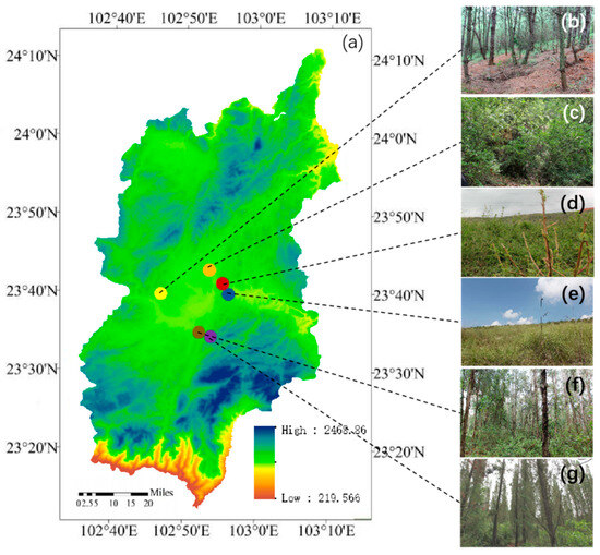
Figure 1.
Distribution map of sampling locations and the study area. (a) DEM map of Jianshui County and location markers of experimental plots, blue indicates high altitude and red indicates low altitude, (b) cypress plantation (Platycladus orientalis), (c) natural secondary forest, (d) mulberry bushes (Dodonaea viscosa), (e) natural grassland, (f) Yunnan pine plantation (Pinus yunnanensis), (g) eucalyptus plantation (Eucalyptus maideni).
2.2. Sample Plot Setting
2.2.1. Vegetation Survey
The stratified survey statistics of trees, shrubs and herbs were carried out in each observation plot (Table 1). In the six experimental areas, a 10 m × 10 m tree quadrature, 5 m × 5 m shrub quadrat, and 1 m × 1 m herb quadrat were selected using the field method, and the canopy closure of the trees in the quadrature was measured. The coverage of shrubs and the coverage of herbs were recorded, and the vegetation characteristics of each test site were analyzed on the basis of calculated relative density (coverage). The relative density (Dr/%) formula is as follows:
where ni is the number of individuals (strains) of a certain tree species, and n is the number of tree species.

Table 1.
Vegetation survey form in the experimental area.
2.2.2. Soil Survey
Experimental plots were selected at the downslope positions in the six types of forestland surveyed above, and three soil samples were collected at depths of 0–10 cm, 10–20 cm, and 20–30 cm. According to the method of Kan et al. (2020) [3], soil property data were obtained (Table 2).
Table 2.
Location of sample plots and soil properties (average value ± standard deviation).
2.3. Soil Column Collection and X-ray CT Scanning
A total of 18 undisturbed soil pillars (inner diameter of 10 cm and height of 30 cm) were collected in six typical vegetation test areas. The nearby CT scanning agency was contacted to complete the scanning of all undisturbed soil columns as soon as possible to avoid disturbance of the soil columns, and the matching data processing software (VG Studio MAX 2.2) was used to perform a 3D reconstruction of the scanned data to obtain the spatial structure of soil pores. It should be noted that, given that the metal pipe wall would affect scanning results, the PVC pipe with a pipe wall thickness of 5 mm was used for acquisition. The mechanical force would cause considerable damage to soil structures. Thus, a sawtooth, a shovel and other tools combined with manual pressing (Figure 2a) were used to peel off excess soil and gravel on the outer wall of the PVC pipe layer by layer. This method facilitates the collection of undisturbed soil columns [13]. The CT scan results show that this method can be used for soil structure studies in this area (Figure 2b).
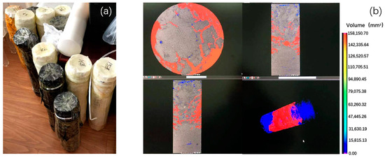
Figure 2.
Soil column collection and X-ray CT scanning. (a) Undisturbed soil column, (b) data processing interface by VG Studio MAX 2.2, the color indicates the pore volume size, red indicates the pore volume close to 160,000 mm3, and blue indicates the pore volume close to 0 mm3.
2.4. Quantitative Description of 3D Soil Macropores
The images processed by VG Studio MAX 2.2 software were statistically analyzed using the particle analysis module (Analyse Particles Tool) of Image J 2x software, and the average diameter of large pores (d/mm), pore volume (Vm/mm3), and pore surface area (Sm/mm2), angle (θ), torsion (ξ), tortuosity (δ), actual length of large pores (Lti) and other characteristic parameters were obtained. In this study, the pores connected to the soil layer with a depth of more than 10 cm at the same time were named soil macropores, and the spatial structure characteristics of such soil macropores will be analyzed in subsequent studies.
In order to quantitatively study the characteristics of the soil macropore spatial structure, on the basis of the topology principle, pore direction was represented by the three-dimensional coordinate axis; that is, a topological pipeline network was obtained and combined with the idea of differentiation. A large pore was infinitely divided into n layers, the pore was regarded as a multi-segment line segment, and the integral calculation of the x, y and z coordinate differences of each line segment was obtained using the characteristic index of the large pore.
Among them, the macropore angle (θ) is defined as the inclination angle of the macropore branch [18], which cannot be directly obtained by the software; therefore, the angle of each layer of macropores is calculated using formula (2):
where x, y and z are the projected macropore lengths in the x, y and z directions, respectively.
The degree of distortion (ξ) is defined as the cumulative value of the angle (θi) of the i-th layer of macropores in the soil with the actual length L0, with a total of n layers. To describe the degree of distortion of macropores in the soil, formula (3) is used to calculate the degree of distortion:
Assuming that each micro-segment of pores is a cylinder after the macropores are split, it can be obtained by using the ratio of volume (V) to upper and lower surface areas (S). Formula (4) is used to calculate the actual length (Lti) of the i-th layer macropores:
The tortuosity (δ) can represent the degree of convolution of the macropore path, which can reflect the length of the migration path of the flowing objects in the macropore channel. Formula (5) is used to calculate the cumulative tortuosity:
where Lti is the actual macropore length (mm) in the i-th layer, and Lli is the vertical distance length (mm) in the i-th layer.
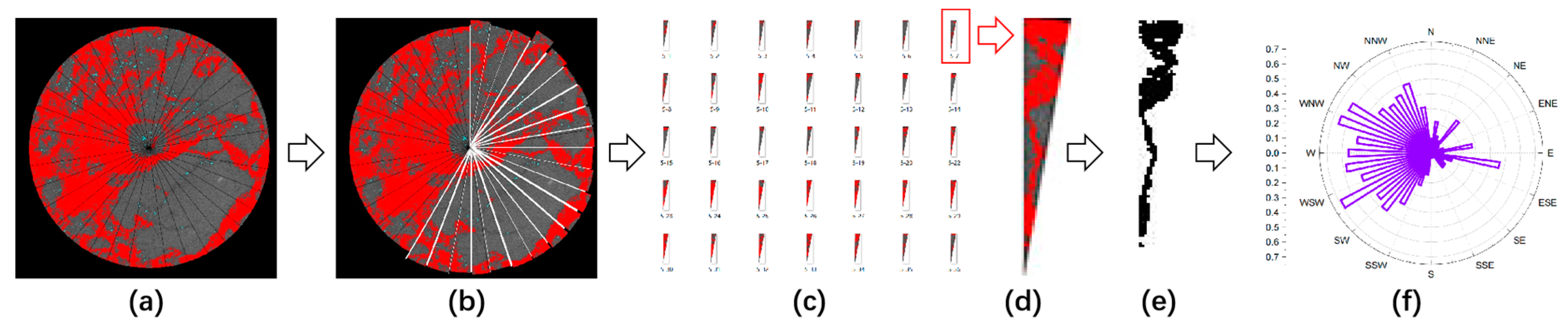
In order to quantify the spatial distribution characteristics and vertical connectivity of soil pores, we adopted the preferential flow research method [3] (Figure 3). Firstly, Adobe Photoshop CS6 was used to scan the cross-sectional images of each layer of the undisturbed soil column for geometric correction and color adjustment. The images were evenly divided into 36 sectors, with each sector area at 10° (Figure 3a), and each sector area was cropped separately (Figure 3b). Each cross-sectional scanning image can obtain 36 sector area maps (Figure 3c). IPWIN Image Pro Plus 6.0 was used to process the cropped sector maps (Figure 3d) and mark the large hole areas in each sector with black (pixel value 0) and the non-hole areas with white (pixel value 255) (Figure 3e), derive a binary matrix, and calculate the large hole areas (pore area ratio) in each sector. Finally, the Origin 2019b software was used to draw a graph based on the fan position (Figure 3f), analyze the morphology and distribution characteristics of the macropores, and calculate the vertical connectivity of the preferential path.

Figure 3.
X-ray CT scanning cross-section image processing process. (a) Horizontal profile screenshots of undisturbed soil columns with CT scans, (b) segmentation of horizontal profile screenshots, (c) all images of an equally segmented horizontal profile, (d) one of the equally segmented fan-shaped images, (e) the large and non-large pores in the equally segmented fan-shaped images are marked black and white, respectively, and the area proportion of macropores in sector images was calculated, (f) the area proportion of macropores in all sector images in this horizontal profile was statistically analyzed.
The formula for calculating the proportion of macropore distribution (Ss) for each sector slice is:
where Ss is the proportion of macropore distribution in each sector slice (%), Xi is the number of macropore-stained pixel grids, r is the number of pixels in the sector radius.
2.5. Water Penetration Simulation Test
The solution permeation simulation test was carried out for the saturated 18 undisturbed soil column, and NaCl was used (Sinopharm Chemical Reagent Co. Ltd., Shanghai, China). [35]. During the experiment, a 15 mm water head was maintained. To ensure the reliability of the test, we carried out only one water infiltration test on each soil column.
The contribution level of the data in this study was analyzed using SEM, and the specific method was shown in Kan et al. (2019) [36].
SEM is widely used due to its empirical analysis capabilities and suitability for latent variable analysis. SEM introduces latent variables that can simultaneously consider endogenous variables, which can allow errors of measurement in parameter estimation whilst analyzing the direct and indirect effects between variables. The structural equation model can obtain the correlation coefficient between the factors, show the directivity of the correlation relationship and calculate the logical relationship between the indicators. The SEM method consists of structural equations and measurement models that are generally represented by three matrix equations, as follows.
η = Bη + Γξ + ζ,
Equation (7) represents SEM, which reflects the structural relationships between latent variables that cannot be measured in practice. Where η is the endogenous latent variable, B is the correlation coefficient matrix between endogenous latent variables, Г is the structural coefficient matrix of exogenous latent variables on endogenous latent variables, ξ is an exogenous latent variable, and ζ is the measurement error.
Y = Λy η + ε
X = Λx ξ + σ.
Equations (8) and (9) represent the measurement models, which can reflect the relationship between observed and latent variables, where X is the exogenous observation variable vector; Y is the endogenous observation variable vector; Λx is the factor loadings of the exogenous observation variable vector; Λy is the factor loadings of endogenous observation variable vector; ε and σ are the measurements of the exogenous and the endogenous observation variables, respectively. Latent variables can be reflected by measurable variables by the use of a measurement model. We can obtain the relationship between each latent variable and measurable variable by solving Equations (7)–(9). After building the initial model, the path coefficients represent the extent of the relationship between the variables. The path coefficients are usually calculated by using the maximum likelihood method.
3. Results
3.1. Spatial Structure Characteristics of Soil Pores
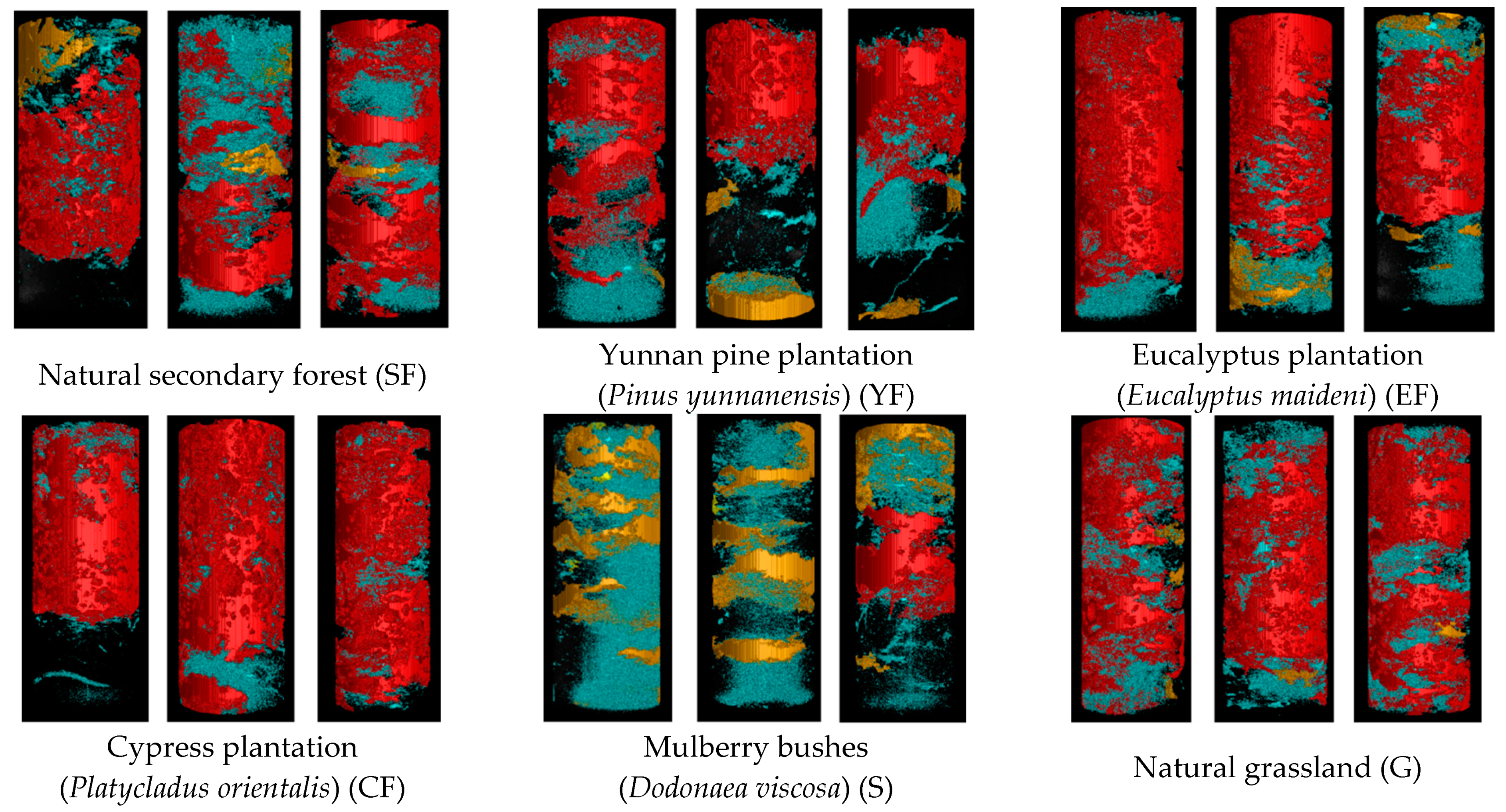
The 3D morphological characteristics of soil pores in undisturbed soil column samples from six typical vegetation types are shown in Figure 4. The macropores showed vertical connectivity, especially macropores with volumes of ≥100,000 mm3, which connected the surface (1 cm) and deep (29 cm) soils, and their morphology, connectivity, distribution and development vary with vegetation type. The volume, number and morphological characteristics of macropores differ significantly with increasing depth. This finding indicated that the largest vertically connected pore is the key path connecting the surface and deep soil. To study 3D distribution at each undisturbed soil columns, we need to classify the soil pores. Since the scan results showed clear stratification at 100,000 mm3 and 5 mm3, we divided soil pore volume (V) into V ≥ 100,000 mm3 (Figure 4 red part), 5 mm3 ≤ V < 100,000 mm3 (Figure 4 yellow part), and V < 5 mm3 (Figure 4 blue part) groups. The average soil macropore volume of SF, YF, EF, CF, S, and G were 252,733.56 mm3, 142,296.14 mm3, 338,404.29 mm3, 143,101.45 mm3, 142,231.18 mm3, 288,412.56 mm3. Among the 18 undisturbed soil columns, the smallest macropore volume was 142,201.48 mm3.
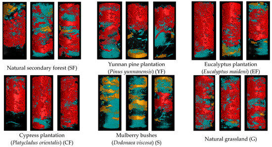
Figure 4.
3D visualization images of undisturbed soil column samples under typical vegetation types. Three undisturbed soil column samples were collected for each planting type. Red part means V ≥ 100,000 mm3, yellow part means 5 mm3 ≤ V <100,000 mm3, and blue part means V < 5 mm3.
Images obtained through CT scanning can reflect the internal structural characteristics of soil. The pores of natural vegetation (SF and G) soil were evenly distributed in the 0–30 cm depth soil, and most macropores (red part) connecting the 0 cm and 30 cm soil, and fewer rhizoidal channels exist. Most of the macropores (red part) in artificial vegetation (YF, EF and CF) soil decreased with the increase in depth; the rhizoidal channels were mainly distributed in 20–30 cm depth and mostly in the horizontal direction. The vertical connectivity of macropores (red part) in planted shrub soil was small and mainly distributed at 0–20 cm depth, and there were more micropores (blue part) with uniform distribution.
3.2. Quantitative Characteristics of Soil Pores
3.2.1. Volume and Quantity Proportion
The total quantity of soil pore with V < 5 mm3 was more than 99% under six vegetation types, and each undisturbed soil column had only one soil pore with V ≥ 100,000 mm3. The number of soil pores (V < 5 mm3 and 5 ≤ V < 100,000 mm3) under the condition of artificial vegetation (YF, EF, CF, S) was about twice that of natural vegetation (SF and G). The number of V < 5 mm3 under S accounts for the largest proportions, reaching 99.85%. The number of 5 ≤ V < 100,000 mm3 under CF accounts for the largest proportions, reaching 0.63%.
The total volume of soil pores with V < 5 mm3, 5 ≤ V < 100,000 mm3 and V ≥ 100,000 mm3 were 5.65%, 10.36% and 83.99% under six vegetation types. The total volume of soil pores with V < 5 mm3 under the condition of artificial vegetation (YF, EF, CF, S) was about twice that of natural vegetation (SF and G), and the total volume of soil pores with 5 ≤ V < 100,000 mm3 under the condition of artificial vegetation (YF, EF, CF, S) was 26.62 times that of natural vegetation (SF and G). The total volume of soil pores with V ≥ 100,000 mm3 under the condition of artificial vegetation (YF, EF, CF, S) was 15.27% of natural vegetation (SF and G).
3.2.2. Diameter and Surface
The mean diameters of soil macropores are similar and show no significant differences (Table 3). SF is larger than the artificial forestland, and the average diameter of macropores in the forestland is about 1.33 times that of S and 1.87 times that of G (natural grassland). Natural vegetation (SF and G) have more soil pore channels than artificial forests, and their average diameters are larger than the average diameter of the artificial forest. The total volume of soil pores in G (natural grassland) is smaller than that of EF, but the total surface area is larger than that of EF, indicating that the distribution of macropores in G (natural grassland) is more dispersed. In the artificial forestland, the total soil pore volume of EF is about two times that of YF (Yunnan pine plantation) and CF, and the total soil pore surface area is about 1.5–2.5 times that of YF (Yunnan pine plantation) and CF, indicating that EF has more soil macropores than YF (Yunnan pine plantation) and CF.
Table 3.
Preferential path characteristic parameters under typical vegetation types.
3.2.3. Curvature and Twist
The pore curvatures of natural vegetation (SF and G) are about 1.18–1.30 times the pore curvature of artificial forestlands (YF, EF, CF and S), and the cumulative distortion of artificial forestland is about 1.30 times that of natural vegetation (SF and G) (Table 4). Natural vegetation (SF and G) have the largest pore curvatures and the smallest pore distortion, indicating that the degree of convolution of the soil macropores of a native forestland is higher than that of an artificial forestland, and the soil macropores for surface water and material transport are long.
Table 4.
Preferential path curvature and cumulative twist under typical vegetation types.
3.2.4. Vertical Connectivity
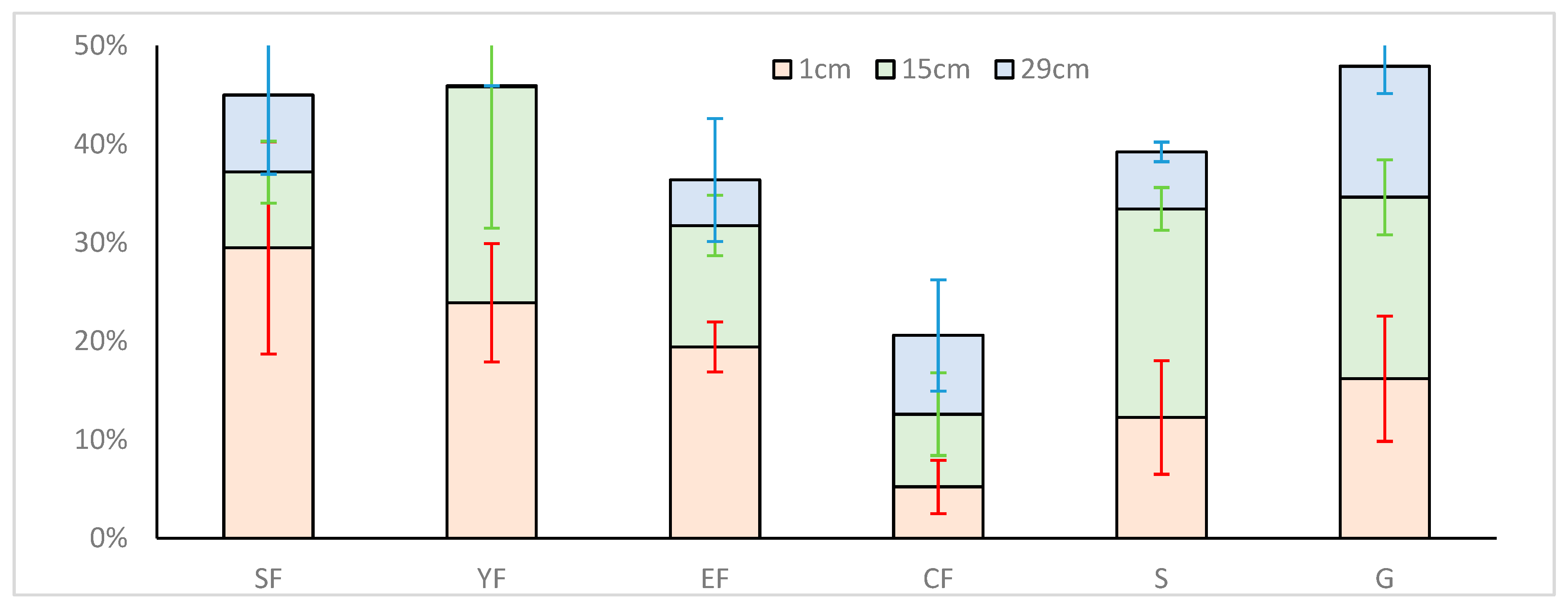
In this study, the vertical connectivity of soil macropores was calculated using pixel processing technology, which obtained horizontal cross-section images by scanning slices. Since pores with V > 100,000 mm3 connect both 0 cm and 30 cm soil, and only one exists in each soil column, it is considered that pores with V > 100,000 mm3 are the preferred path for water migration in shallow soil and vertical connectivity is calculated for this part of the pores. The sequence of the average proportion of large pores in the horizontal section is as follows (Figure 5): G (47.93%) > YF (45.94%) > SF (45.02%) > S (39.23%) > EF (36.38%) > CF (9.64%). The proportions of macropores in the horizontal section of the artificial forestlands decrease with increasing depth. The degree of connectivity (τ) of SF, G, YF, EF, CF and S was calculated using Equation (6): 72.05% (SF), 75.68% (G), 77.21% (YF), 25.37% (EF), 18.60% (CF) and 71.83% (S). The average degree of connectivity of an artificial forestland in karst areas is 34.68% smaller than that of natural vegetation (SF and G). This difference is mainly due to artificial revegetation, which has changed the soil structure, and the degree of soil connectivity of the artificial forestland is greatly reduced. EF is 64.77% lower than SF and 66.62% lower than the G (natural grassland). CF is 74.17% lower than SF and 75.53% lower than G (natural grassland). S is 0.23% lower than SF and 5.48% lower than G (natural grassland).

Figure 5.
The proportions of macropores in the horizontal section of different typical vegetation types. 1 cm, 15 cm, and 29 cm, respectively, represent the proportion of soil macropores in the horizontal section at a vertical distance of 1 cm, 15 cm, and 29 cm from the surface of the undisturbed soil column, the corresponding standard deviations are marked with red (1 cm), green (15 cm), and blue (29 cm) lines. The bar chart is the average of 3 samples, and the line segments are the standard deviations of 3 samples under the condition of agreeing vegetation type.
3.3. Effect of Soil Porosity on Water Transport
To study the preferential flow process under different vertical connectivity of soil pores, a water infiltration simulation was carried out on the undisturbed soil column after scanning (Table 5). The speed of vertical water migration and change in solution conductivity increases with the vertical connectivity of soil pores. As the degree of pore connectivity decreases, the hysteresis of the outflow from the bottom becomes increasingly obvious when water is added for the first time, and the stabilization time of electrical conductivity accounts for a large proportion of the total test duration. The total test durations corresponding to the vertical connectivity in ranges of 10–20, 20–40 and 40–60 is 20.31, 24.80, and 31.46 times the total test duration in 0–10, indicating that the time that water travels to the 30 cm depth through vertical infiltration increases with the decreasing vertical connectivity of soil pores. After the solution was added, the change process of the conductivity at the bottom of the soil column shows hysteresis and the time to reach stability accounts for a large proportion of the total test duration.
Table 5.
Simulation of solute transport in undisturbed soil column under six vegetation types.
According to the vertical connectivity, we divided 18 undisturbed soil columns into different levels: 0 < τ < 10, 10 < τ < 30, 30 < τ< 50 and 50 < τ< 70 to clearly count and analyze the simulation results of water migration. The speed of vertical water migration and change in solution conductivity increases with the vertical connectivity of soil pores. As the degree of pore connectivity decreases, the hysteresis of the outflow from the bottom becomes increasingly obvious when water is added for the first time, and the stabilization time of electrical conductivity accounts for a large proportion of the total test duration. The total test durations corresponding to the vertical connectivity in the ranges of 10–20, 20–40 and 40–60 is 20.31, 24.80, and 31.46 times the total test duration in 0–10, indicating that the time that water travels to the 30 cm depth through vertical infiltration increases with the decreasing vertical connectivity of soil pores. After the solution was added, the change process of the conductivity at the bottom of the soil column shows hysteresis and the time to reach stability accounts for a large proportion of the total test duration.
The sum of “add water after saturation-total time”, “add 25 ms/cm NaCl solution 2000-mL total time”, “add water after saturation-total time” for each undisturbed soil column is water transport total stable time (TT), the average of “add water after saturation-average water transport velocity and average change rate of conductivity”, “add 25 ms/cm NaCl solution 2000-mL average water transport velocity and average change rate of conductivity”, “add water after saturation -average water transport velocity and average change rate of conductivity” for each undisturbed soil column is average water transport velocity (WTV) and electrolyte change rate (ARC). These data will be used to study the correlation between soil pore characteristics and water transport.
3.4. Structural Equation Model (SEM) Analysis
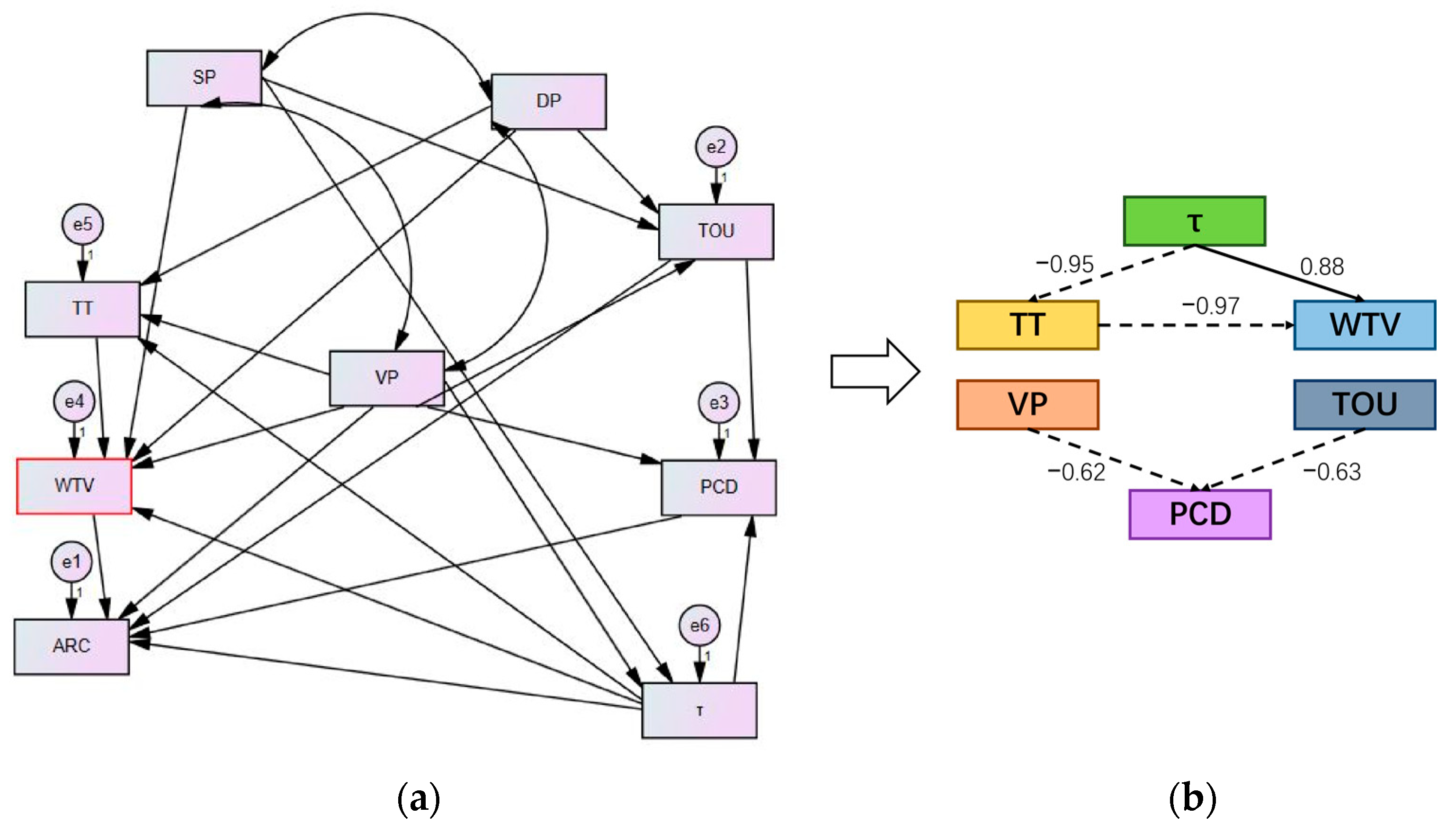
In order to study the relationship between soil vertical connected pores and water transport, the Structural Equation Model (SEM, Section 2.5) was used to analyze the soil pore index and water transport index (Figure 6). The soil porosity index includes the total volume (VP), surface area (SP), average diameter (DP), tortuosity (TOU), porosity distortion (PCD), vertical connectivity (τ), and water transport index includes water transport total stable time (TT), average water transport velocity (WTV), and electrolyte change rate (ARC). Compared with the traditional Pearson correlation coefficient statistical method, SEM considers measurable variables and potential variables separately in the process of correlation analysis, allowing measurement errors (ei in Figure 6) in parameter estimation and reducing the interference caused by measurement errors in correlation estimation among potential variables, and the arrows between the indexes were the causality of the related path.

Figure 6.
Covariance results of SEM variables. (a) SEM model structure of all indexes, (b) The actual correlation of 6 indicators and their correlation screened by SEM model, the numbers above the arrows represent correlations. The arrow between (a,b) indicates the running and screening of the SEM model.
The τ value has a significant negative correlation with the TT of water transport (normalized estimate is −0.95) and has a significant positive correlation with the WTV of water transport (normalized estimate is 0.88). These correlations indicate that the vertical migration speed of water per unit volume increases with the degree of vertical connectivity in soil pores. The VP and TOU of soil pores are significantly negatively correlated with PCD (normalized estimates are −0.62 and −0.63, respectively), indicating that PCD increases, whereas the degree of twisting of porosity decreases with increasing soil pore volume and degree of tortuosity.
4. Discussion
4.1. Soil Pore Morphology
The spatial structure characteristics of soil macropores’ preferential paths affect soil moisture preferential transport capacity. The soil preferential paths are defined as the large pores that connect the surface and deep soil. However, no unified conclusion on the classification standard of soil macropores has been formulated. Therefore, in this study, volume was used for division and determination, which are more conducive to the analysis of the spatial structure characteristics of soil macropores and calculation of the connectivity of soil preferential paths than division methods.
Macropores with volume of ≥100,000 mm3 can connect the surface and 30 cm deep soil layer, and the total volume ratio is close to 100 times that of the pores with volume of <5 mm3. The volume ratio in soil plays an important role in water transport and provides a pathway [37]. Macropores with volumes of ≥100,000 mm3 in SF (natural secondary forestland) are uniformly distributed and have strong vertical connectivity, forming a transport channel connecting the surface and deep soil [38]. The macropores of G (natural grassland) with volumes of ≥100,000 mm3 are widely and uniformly distributed, showing obvious root channel morphology in the 0–10 cm deep soil layer, but the macropore morphology in the 10–30 cm deep soil layer mainly showed the state of being connected by broken fissures, indicating that the soil structure in the native state is not only affected by the root system of vegetation. Macropores with volumes of ≥100,000 mm3 in the artificial forestland show aggregated morphology, and significant cylindrical root channel macropores are present, which are mainly concentrated in the soil at a depth of 0–20 cm. Soil with a depth of 10–30 cm has an obvious root channel network structure, and the degree of soil fragmentation is lower than that of natural vegetation types (natural secondary forestland, natural grassland); after artificial forest restoration, the reduced number and pore size of soil pore channels may hinder the rapid passage of water and solutes, which can effectively prolong the retention time of water in shallow soil [37]. Transport of water and substances and a large total surface area of soil pores is conducive to the contact and absorption of water and transported substances, effectively increasing the water storage capacity of soil and reducing the time that water stays on the surface [39], reducing water evaporation and promoting the utilization of surface water. Therefore, the surface infiltration rates of water and solute in EF (Eucalyptus plantation) are much higher than those in YF (Yunnan pine plantation) and CF (Cypress plantation).
The distribution of macropores in G (natural grassland) is quite special in southwestern China. The pore structure of grassland in the 0–10 cm deep soil layer is similar to that of grassland soil in other areas because herbaceous roots are mainly distributed in this soil layer, and a large number of soil pores in the shape of root grooves were found. However, the results of CT scanning (Figure 4) showed that in the unrooted zone of 10–30 cm deep soil layer [40], the macropores with volumes of ≥100,000 mm3 are still widely distributed, which indicates that the soil pore structure of G (natural grassland) in this area is special. In 10–30 cm deep soil layer, the macropore morphology is mainly in the state of being connected by broken fissures, and they are independent of each other, and no obvious root channel shape is present. Therefore, different from the soil pores of grassland in Beijing or Chongqing [20,41], which are concentrated in the 0–10 cm soil layer, the soil pores of natural grassland in Yunnan Province in this study are widely distributed in the 0–30 cm soil layer, which is conducive to the rapid infiltration and migration of surface water into deeper soil layers.
The lateral connectivity of S (mulberry bushes) is strong, mainly developed laterally and has a relatively uniform distribution, similar to the research results of Kung et al. (1990) [42]. This type of soil macroporosity easily forms the lateral preferential flow of water, which reduces the stability of the covering soil [43]. This state is conducive to the lateral connection of the soil and the lateral flow of soil moisture but reduces the stability of the covering soil [44]. Pores with volumes lower than 5 mm3 are uniformly distributed and do not change with depth and are thus conducive to long-term soil water storage and promote the growth of vegetation roots.
4.2. Vertical Connectivity of Soil Pores
In terms of macropore characteristic parameters, the development degree of soil macropores preferential path under typical vegetation conditions is calculated using the topology principle, and the 3D spatial morphological characteristics of macropores are quantified as the average diameter (d/mm) and the total volume (Vm/mm3); total surface (Sm/mm2), twisty (ξ), tortuosity (δ) and other characteristic parameters are used to evaluate the development degree of soil macropores’ preferential path under typical vegetation conditions [18]. Under typical vegetation conditions, the average diameter (d/mm) of soil macropores in adjacent soil layers was not significantly different. Among them, natural vegetation types (natural secondary forestland, natural grassland) have more soil pore channels than artificial forestland, and the average diameter is also larger than that of artificial forestland. However, Guo et al. (2018) [45] considered the soil pore structure of natural vegetation types (natural secondary forestland, natural grassland) to be more conducive to the occurrence of soil preferential flow. The total volume (Vm/mm3) of G (natural grassland) is smaller than that of the EF (eucalyptus plantation), but the total surface area is larger than that of the EF (Eucalyptus plantation), indicating that the distribution of macropores in G (natural grassland) soil is relatively scattered. In the artificial forest, the number of macropores in the EF (Eucalyptus plantation) is more than that in the YF (Yunnan pine plantation) and the CF (Cypress plantation). It is beneficial to increase the contact of soil with water and its transported substances. Therefore, the soil of artificial forestland has a high degree of contact with infiltrated water and substances, which is beneficial to the improvement of water and substances transport in soil. At the same time, natural vegetation types (natural secondary forestland, natural grassland) have the largest pore curvature and the smallest pore distortion, indicating that the convolution degree of soil macropore paths in natural vegetation types (natural secondary forestland, natural grassland) is higher than that in artificial forestland, and surface water and materials are transported in soil macropore channels, the preferential path is longer [21].
On macropore tendency, macropores have an obvious tendency under all vegetation type conditions. However, different from the results of Collon et al. (2017) [46] is the asymmetry of fissures in the soil of subslope vegetation. The proportion of macropores at different depths and their angles are similar under typical vegetation types, indicating that the positions of macropores in the upper, middle and lower soil layers within a unit soil column volume are related to each other, and macropores have vertical connectivity [18]. The correlation between the distribution locations of natural vegetation types (natural secondary forestland, natural grassland) and macropores is greater than that in planted forestlands, showing that the preferential path trends of soil macropores in natural vegetation types (natural secondary forestland, natural grassland) soils are consistent in different soil layers. Meanwhile, soil macropore trends in artificial forestlands are dispersed. Compared with the macropore trend morphological character of the two forestlands, the macropores of SF (natural secondary forestland) are more heterogeneous, whereas the distribution of macropores in the plantation is more uniform, and the degree of bias is high. The proportion of macropores in soil layers with different depths is quite different, and the proportion of macropores in forestlands decreases with increasing depth. No root system is present in the 10–30 cm deep soil layer of natural grassland. This mode of formation is conducive to the storage of water in the soil and promotes the development of deep soil fissures. Comparing the proportions of macropores in different soil layers, this study found that the proportions of large pores in the horizontal section of SF (natural secondary forestland) at depths of 1, 15 and 29 cm are 29.49%, 7.69%, and 7.83%, respectively. In the horizontal section of G (natural grassland) at depths of 1, 15 and 29 cm, the proportions of large pores are 16.21%, 18.42% and 13.30%, respectively.
Developmental characteristics, such as macropore volume and surface area in soil, determine soil connectivity [13]. However, research on the calculation of soil macropore connectivity mainly focuses on the calculation of soil column simulation infiltration rate and staining area ratio, and accurately reflecting and objectively describing the degree of soil macropore connectivity is difficult. Therefore, the degree of vertical connectivity degree (τ) of the soil’s preferential path was calculated using the rose diagram of the proportion of macropores with volumes of ≥100,000 mm3 at different soil depths. This method of quantitatively evaluating the vertical connectivity difference of soil macropores in typical vegetation types complements the research method of preferential paths [44].
4.3. Contribution of Soil Pore Vertical Connectivity to Water Transport
Many studies and simulations of soil solute transport processes are mainly concentrated in farmlands. The total time of soil column water migration in the artificially restored vegetation environment in Table 5 is twofold that of the natural vegetation environment, and the outflow rate and electrolyte changes at 30 cm depth are 0.56 and 0.86 times those of a natural vegetation environment, respectively. This finding shows that the soil pore structure is the key factor for water loss in the natural vegetation environment, and the soil pore structure after the artificial restoration of vegetation has changed. According to the change in the vertical connectivity of the pores, the mitigation of water loss at 30 cm depth is achieved. It does not hinder the infiltration of surface water and can facilitate water storage in shallow soil in a short time. Therefore, for the water loss problem of the surface soil in the karst area, the artificial restoration of vegetation can alleviate surface water loss and leakage, improve the water retention capacity of the 0–30 cm shallow soil and provide water protection for the growth of shallow root vegetation.
Although water transport in soil has been extensively studied, current research mainly focuses on the simulation and verification of models and detection with intelligent instruments [47]. The basic indicators are always visually observable data. The link between soil structure and water transport needs further study. SEM analysis shows that this method can be used as a link between soil pore structure and water transport results and provides a novel approach for further research on the mechanism of water transport in the vadose zone of the soil. In water transport in solution-simulated undisturbed soil, electrolyte-altered hysteresis and loss occur, similar to the results of the Cl− soil column simulation of Kadyampakeni et al. (2018) [48] and different from the results of 15NO3− adsorption experiments in sandy farmland soils [49]. This may be due to the fact that the transport process of ions in soil is related to ion types. Therefore, in the study of soil water loss and non-point source pollution, systematic simulation and verification of specific ions are required.
5. Conclusions
This study analyzed and compared the soil pore structure, vertical connectivity of soil macropores, characteristics of water preferential movement and their contributions under six typical vegetation conditions in southwestern China through CT scanning of undisturbed soil columns and water infiltration simulation test. The results revealed that the number of pores with a volume between 5 mm3 and 100,000 mm3 (including 5 mm3) was relatively small and mainly distributed in the vertical direction under natural vegetation (natural secondary forestland, natural grassland) conditions, a large number of pores with a volume ranging from 5 mm3 to 100,000 mm3 (including 5 mm3) mainly distributed in the horizontal direction under artificial forestland (YF, EF, CF), which were concentrated in soil at a depth of 10–30 cm and exhibited a root channel-like structure. The macropore distribution area of artificial forestland in surface soil (1 cm), intermediate soil (15 cm) and deep soil (29 cm) layer was 33.45%, 20.21% and 56.15% less than natural vegetation, respectively, thus improving the water retention capacity of the soil. The soil porosity of artificial restoration forestland was significantly reduced, which could promote local soil water retention and reduce the rapid loss of surface water. The average connectivity of artificial restoration forestland was 34.68% lower than that of natural vegetation, and artificial forestland effectively reduces the vertical connectivity of large pores in shallow soil. Therefore, plantation restoration can reduce the development of desertification, improve the surface soil pore structure, reduce vertical connectivity by nearly 20%, reduce water efflux rate at a depth of 30 cm by nearly 44% and reduce the change in electrolyte content by nearly 14%. When the degree of soil vertical connectivity increases from 0–10 to 10–30, 30–50 and 50–70, the time required for water to penetrate a 30 cm soil column to stabilize flow and electrolyte is shortened by 21%, 35% and 97%, respectively. The degree of vertical connectivity of soil pores is significantly negatively correlated with the total time of stabilization of water transport (the normalized estimate is −0.95) and significantly positively correlated with the average flow rate of water transport (the normalized estimate is 0.88). The degree of soil vertical connectivity can facilitate the quantitative description of soil pore structure and realize the comprehensive study of soil structure and water transport. The calculation method for vertical connectivity of soil macropores can provide a new method for subsequent research on water conservation and preferential flow in forestland, and this study will hopefully provide data and method foundation for the restoration and protection of local forestland. The results of this study demonstrate that vegetation restoration in this region will improve local soil water conservation capacity. It is recommended to further improve vegetation restoration projects and consider increasing tree species, such as economic forests, to provide economic value for the local people while maintaining soil and water. However, this study only collected four types of artificially restored vegetation. In the next step of the study, the soil pore spatial structure and its contribution to water transport under the conditions of local reclaimed tree species such as Amorpha fruticosa, Chinese fir, Huashan pine, and Cypress can be studied. And the water transport simulation model for local soil pores can be constructed to clarify the degree of soil and water conservation after local vegetation restoration and provide a theoretical basis and data guidance for the long-term development of local vegetation restoration projects.
Author Contributions
Conceptualization, X.K. and J.C.; methodology, X.K.; software, X.K. and W.Z.; validation, X.K., L.Z. and J.L.; formal analysis, X.K.; investigation, X.K.; resources, X.K.; data curation, X.K.; writing—original draft preparation, X.K.; writing—review and editing, X.K. and B.L.; visualization, X.K.; supervision, X.K.; project administration, X.K. and X.Z.; funding acquisition, X.K. All authors have read and agreed to the published version of the manuscript.
Funding
This research was funded by the National key research and development program (2021YFD1000205), the Yunnan key research and development program (202002AE090010), National Natural Science Foundation of China (32071839), Beijing Postdoctoral Research Foundation (2023-ZZ-115), Postdoctoral Research Foundation of Beijing Academy of Agriculture and Forestry Sciences (2022-ZZ-005).
Data Availability Statement
Not applicable.
Acknowledgments
Many thanks to the JianShui Forestry Station for offering accommodation and supporting field experiments. Meanwhile, we gratefully acknowledge the editor and reviewers.
Conflicts of Interest
The authors declare no conflict of interest.
References
- Chen, H.; Li, D.J.; Xiao, K.C.; Wang, K. Soil microbial processes and resource limitation in karst and non-karst forests. Funct. Ecol. 2018, 32, 1400–1409. [Google Scholar] [CrossRef]
- Chen, H.; Hu, K.; Nie, Y. Analysis of soil water movement inside a footslope and a depression in a karst catchment, Southwest China. Sci. Rep. 2017, 7, 2544. [Google Scholar] [CrossRef] [PubMed]
- Kan, X.; Cheng, J.; Hou, F. Response of Preferential Soil Flow to Different Infiltration Rates and Vegetation Types in the Karst Region of Southwest China. Water 2020, 12, 1778. [Google Scholar] [CrossRef]
- Katharina, S.; Andrew, D.; Nico, E.; Kai, U. Depth-differentiated, multivariate control of biopore number under different land-use practices. Geoderma 2022, 418, 115852. [Google Scholar]
- Wand, S.; Li, R.; Sun, C. How Types of carbonate assemblages constrain the distribution of karst rocky desertification in Guizhou Province, P.R. China: Phenomena and mechanism. Land Degrad. Dev. 2004, 15, 123–131. [Google Scholar]
- Palmer, A. Origin and morphology of limestone caves. GSA Bull. 1991, 103, 1–21. [Google Scholar] [CrossRef]
- Karsanina, M.V.; Gerke, K.M.; Skvortsova, E.B.; Mallants, D. Universal spatial correlation functions for describing and reconstructing soil microstructure. PLoS ONE 2015, 10, e0126515. [Google Scholar] [CrossRef]
- Hallett, P.D.; Feeney, D.S.; Bengough, A.G.; Rillig, M.C.; Scrimgeour, C.M.; Young, I.M. Disentangling the impact of AM fungi versus roots on soil structure and water transport. Plant Soil 2009, 314, 183–196. [Google Scholar] [CrossRef]
- Zhang, Z.B.; Zhou, H.; Zhao, Q.G.; Peng, X. Characteristics of cracks in two paddy soils and their impacts on preferential flow. Geoderma 2014, 228, 114–121. [Google Scholar] [CrossRef]
- Köhne, J.M.; Köhne, S.; Šimůnek, J. A review of model applications for structured soils: a) Water flow and tracer transport. J. Contam. Hydrol. 2009, 104, 4–35. [Google Scholar] [CrossRef]
- Köhne, J.M.; Schlüter, S.; Vogel, H.J. Predicting solute transport in structured soil using pore network models. Vadose Zone J. 2011, 10, 1082–1096. [Google Scholar] [CrossRef]
- Batany, S.; Peyneau, P.E.; Lassabatère, L.; Béchet, B.; Faure, P.; Dangla, P. Interplay between Molecular Diffusion and Advection during Solute Transport in Macroporous Media. Vadose Zone J. 2019, 18, 1–15. [Google Scholar] [CrossRef]
- Jarvis, N. A review of non-equilibrium water flow and solute transport in soil macropores: Principles, controlling factors and consequences for water quality. Eur. J. Soil Sci. 2007, 58, 523–546. [Google Scholar] [CrossRef]
- Wang, C.; Wang, R.; Huo, Z.; Xie, E.; Dahlke, H.E. Colloid transport through soil and other porous media under transient flow conditions—A review. Wiley Interdiscip. Rev. Water 2020, 7, e1439. [Google Scholar] [CrossRef]
- Sander, T.; Gerke, H.H. Preferential flow patterns in paddy fields using a dye tracer. Vadose Zone J. 2007, 6, 105–115. [Google Scholar] [CrossRef]
- Jarvis, N.; Koestel, J.; Larsbo, M. Understanding preferential flow in the vadose zone: Recent advances and future prospects. Vadose Zone J. 2016, 15, 1–11. [Google Scholar] [CrossRef]
- Kaufmann, G. Modelling karst aquifer evolution in fractured, porous rocks. J. Hydrol. 2016, 543, 796–807. [Google Scholar] [CrossRef]
- Zhang, X.; Hu, M.; Guo, X. Effects of topographic factors on runoff and soil loss in Southwest China. Catena 2018, 160, 394–402. [Google Scholar] [CrossRef]
- Guo, L.; Liu, Y.; Wu, G.L.; Huang, Z.; Cui, Z.; Cheng, Z.; Zhang, R.-Q.; Tian, F.-P.; He, H. Preferential water flow: Influence of alfalfa (Medicago sativa L.) decayed root channels on soil water infiltration. J. Hydrol. 2019, 578, 124019. [Google Scholar] [CrossRef]
- Meng, C.; Niu, J.Z.; Li, X.; Luo, Z.; Du, X.; Du, J.; Lin, X.; Yu, X. Quantifying soil macropore networks in different forest communities using industrial computed tomography in a mountainous area of North China. J. Soils Sediments 2017, 17, 2357–2370. [Google Scholar] [CrossRef]
- Meng, C.; Niu, J.; Yin, Z.; Luo, Z.; Lin, X.; Jia, J. Characteristics of rock fragments in different forest stony soil and its relationship with macropore characteristics in mountain area, northern China. J. Mt. Sci. 2018, 15, 519–531. [Google Scholar] [CrossRef]
- Perret, J.; Prasher, S.O.; Kantzas, A.; Langford, C. Three-dimensional quantification of macropore networks in undisturbed soil cores. Soil Sci. Soc. Am. J. 1999, 63, 1530–1543. [Google Scholar] [CrossRef]
- Noguchi, S.; Tsuboyama, Y.; Sidle, R.C.; Hosoda, I. Morphological characteristics of macropores and the distribution of preferential flow pathways in a forested slope segment. Soil Sci. Soc. Am. J. 1999, 63, 1413–1423. [Google Scholar] [CrossRef]
- Pierret, A.; Capowiez, Y.; Belzunces, L.; Moran, C.J. 3D reconstruction and quantification of macropores using X-ray computed tomography and image analysis. Geoderma 2002, 106, 247–271. [Google Scholar] [CrossRef]
- Mooney, S.J.; Korošak, D. Using complex networks to model two- and three-dimensional soil porous architecture. Soil Sci. Soc. Am. J. 2009, 73, 1094–1100. [Google Scholar] [CrossRef]
- Luo, L.; Lin, H.; Schmidt, J. Quantitative relationships between soil macropore characteristics and preferential flow and transport. Soil Sci. Soc. Am. J. 2010, 74, 1929–1937. [Google Scholar] [CrossRef]
- Nieber, J.L.; Sidle, R.C. How do disconnected macropores in sloping soils facilitate preferential flow? Hydrol. Process 2010, 24, 1582–1594. [Google Scholar] [CrossRef]
- Katuwal, S.; Norgaard, T.; Moldrup, P.; Lamandé, M.; Wildenschild, D.; de Jonge, L.W. Linking air and water transport in intact soils to macropore characteristics inferred from X-ray computed tomography. Geoderma 2015, 237, 9–20. [Google Scholar] [CrossRef]
- Hyväluoma, J.; Thapaliya, M.; Alaraudanjoki, J.; Sirén, T. Using microtomography, image analysis and flow simulations to characterize soil surface seals. Comput. Geosci. 2012, 48, 93–101. [Google Scholar] [CrossRef]
- Scheibe, T.D.; Perkins, W.A.; Richmond, M.C.; McKinley, M.I.; Romero-Gomez, P.D.J.; Oostrom, M.; Wietsma, T.W.; Serkowski, J.A.; Zachara, J.M. Pore-scale and multiscale numerical simulation of flow and transport in a laboratory-scale column. Water Resour. Res. 2015, 51, 1023–1035. [Google Scholar] [CrossRef]
- Francesco, A.; Petrucci, G.; Matzl, M.; Schneebeli, M.; De Michele, C. Early formation of preferential flow in a homogeneous snowpack observed by micro-CT. Water Resour. Res. 2017, 53, 3713–3729. [Google Scholar]
- Larsbo, M.; Koestel, J.; Jarvis, N. Relations between macropore network characteristics and the degree of preferential solute transport. Hydrol. Earth Syst. Sci. Discuss. 2014, 18, 5255–5269. [Google Scholar] [CrossRef]
- Jarvis, N.; Larsbo, M.; Koestel, J. Connectivity and percolation of structural pore networks in a cultivated silt loam soil quantified by X-ray tomography. Geoderma 2017, 287, 71–79. [Google Scholar] [CrossRef]
- Bottinelli, N.; Zhou, H.; Boivin, P.; Zhang, Z.; Jouquet, P.; Hartmann, C.; Peng, X. Macropores generated during shrinkage in two paddy soils using X-ray micro-computed tomography. Geoderma 2016, 265, 78–86. [Google Scholar] [CrossRef]
- Chen, X. Study on characteristics of preferential flow on four land use tupes in Simian Mountain of Chongqing. Beijing For. Univ. 2005, 19, 887–899. [Google Scholar]
- Kan, X.; Cheng, J.; Hu, X.; Zhu, F.; Li, M. Effects of Grass and Forests and the Infiltration Amount on Preferential Flow in Karst Regions of China. Water 2019, 11, 1634. [Google Scholar] [CrossRef]
- Angel, A.A.; Ingrid, P.; Raul, M.; Vesper, D.J.; Meeker, J.D.; Alshawabkeh, A.N. Estimating preferential flow in Karstic aquifers using statistical mixed Models. Ground Water 2014, 52, 584–596. [Google Scholar]
- Green, R.T.; Bertetti, F.T.; Miller, M.S. Focused groundwater flow in a carbonate aquifer in a semi-arid environment. J. Hydrol. 2014, 517, 284–297. [Google Scholar] [CrossRef]
- Yang, J.L.; Zhang, G.L. Water infiltration in urban soils and its effects on the quantity and quality of runoff. J. Soils Sediments 2011, 11, 751–761. [Google Scholar] [CrossRef]
- Dusek, J.; Vogel, T. Modeling subsurface hillslope runoff dominated by preferential flow: One- vs. two-dimensional approximation. Vadose Zone J. 2014, 13, 1–13. [Google Scholar] [CrossRef]
- Chen, X.; Cheng, J.; Zhang, H. Application of landscape pattern analysis to quantitatively evaluate the spatial structure characteristics of preferential flow paths in farmland. Appl. Eng. Agric. 2016, 32, 203–215. [Google Scholar]
- Kung, K.J.S. Preferential flow in a sandy vadose zone: 1. Field observation. Geoderma 1990, 46, 51–58. [Google Scholar] [CrossRef]
- McDonnell, J.J. A rationale for old water discharge through macropores in a steep, humid catchment. Water Resour. Res. 1990, 26, 2821–2832. [Google Scholar] [CrossRef]
- Peng, T.; Wang, S.J. Effects of land use, land cover and rainfall regimes on the surface runoff and soil loss on karst slopes in southwest China. Catena 2012, 90, 53–62. [Google Scholar] [CrossRef]
- Guo, L.; Lin, H. Addressing two bottlenecks to advance the understanding of preferential flow in soils. Adv. Agron. 2018, 147, 61–117. [Google Scholar]
- Collon, P.; Bernasconi, D.; Vuilleumier, C.; Renard, P. Statistical metrics for the characterization of karst network geometry and topology. Geomorphology 2017, 283, 122–142. [Google Scholar] [CrossRef]
- Lai, X.; Zhu, Q.; Michael, J.; Liao, K. Soil rock fragments: Unquantified players in terrestrial carbon and nitrogen cycles. Geoderma 2022, 406, 115530. [Google Scholar] [CrossRef]
- Kadyampakeni, D.M.; Nkedi-Kizza, P.; Leiva, J.A.; Muwamba, A.; Fletcher, E.; Morgan, K.T. Ammonium and nitrate transport during saturated and unsaturated water flow through sandy soils. J. Plant Nutr. Soil Sci. 2018, 181, 198–210. [Google Scholar] [CrossRef]
- Fishkis, O.; Noell, U.; Diehl, L.; Jaquemotte, J.; Lamparter, A.; Stange, C.; Burke, V.; Koeniger, P.; Stadler, S. Multitracer irrigation experiment for assessing the relevance of preferential flow for non-sorbing solute transport in agricultural soils. Geoderma 2019, 371, 114386. [Google Scholar] [CrossRef]

Disclaimer/Publisher’s Note: The statements, opinions and data contained in all publications are solely those of the individual author(s) and contributor(s) and not of MDPI and/or the editor(s). MDPI and/or the editor(s) disclaim responsibility for any injury to people or property resulting from any ideas, methods, instructions or products referred to in the content. |
© 2023 by the authors. Licensee MDPI, Basel, Switzerland. This article is an open access article distributed under the terms and conditions of the Creative Commons Attribution (CC BY) license (https://creativecommons.org/licenses/by/4.0/).