Article

Ungauged Basin Flood Prediction Using Long Short-Term Memory and Unstructured Social Media Data

1
Civil and Environmental Engineering, University of Science & Technology, Daejeon 305-333, Republic of Korea
2
Korea Institute of Civil Engineering and Building Technology, Goyang 10223, Republic of Korea
*
Author to whom correspondence should be addressed.
Water 2023, 15(21), 3818; https://doi.org/10.3390/w15213818
Submission received: 30 September 2023 / Revised: 24 October 2023 / Accepted: 26 October 2023 / Published: 1 November 2023

Abstract

:
Floods are highly perilous and recurring natural disasters that cause extensive property damage and threaten human life. However, the paucity of hydrological observational data hampers the precision of physical flood models, particularly in ungauged basins. Recent advances in disaster monitoring have explored the potential of social media as a valuable source of information. This study investigates the spatiotemporal consistency of social media data during flooding events and evaluates its viability as a substitute for hydrological data in ungauged catchments. To assess the utility of social media as an input factor for flood prediction models, the study conducted time-series and spatial correlation analyses by employing spatial scan statistics and confusion matrices. Subsequently, a long short-term memory model was used to forecast the outflow volume in the Ui Stream basin in South Korea. A comparative analysis of various input factor combinations revealed that datasets incorporating rainfall, outflow models, and social media data exhibited the highest accuracy, with a Nash–Sutcliffe efficiency of 94%, correlation coefficient of 97%, and a minimal normalized root mean square error of 0.92%. This study demonstrated the potential of social media data as a viable alternative for data-scarce basins, highlighting its effectiveness in enhancing flood prediction accuracy.

1. Introduction

Floods are some of the most dangerous and frequent natural disasters that cause property destruction and endanger lives. Among the disasters in the Southwest Pacific region, floods accounted for 78% and 63% of the number of casualties and property damage, respectively [1]. Changes in management methods are essential, given the growing influence of flooding caused by heavy rains and urbanization, which is gradually occurring locally and on a large scale, owing to climate change [2,3]. Using physical data, the hydrological runoff model, which is widely used for flood prediction, can make predictions similar to actual observations. However, the number of high-intensity rainfall events, such as flash floods, continues to increase; thus, existing physical models may not be suitable for flood prediction since obtaining results takes substantial time, owing to the high computational requirements, depending on the size of the model.
Recently, various studies using neural network models for flood prediction have been conducted [4,5,6,7,8,9,10,11,12,13,14,15,16,17,18,19,20,21]. An artificial neural network (ANN) model is a data-driven model that can make predictions rapidly, owing to fewer computational requirements than existing physical models. ANN models can improve the accuracy of predicting hydrological variables, such as water level, flow rate, and precipitation, as they effectively predict nonlinear data [4,5,6,7,8,9,10,11]. Several studies have compared the accuracy of neural network models for outflow prediction [12,13,14]. Dehghani et al. [15] highlighted that a long short-term memory (LSTM) model has the best prediction rate for small basins, whereas convolutional neural network (CNN) and convolutional LSTM (ConvLSTM) models are best for short-term streamflow predictions of 1 h in larger basins. Atashi et al. [16] conducted a similar study, finding that LSTM outperformed 1D-CNN in predicting flood events at the USGS Grand Forks Station. Despite the improved performance of predictive models, their accuracy degrades with a lack of hydrological observational data, and predictions for unmeasured regions remain limited [17,18]. Accordingly, research is actively being conducted to predict the flow rate of unmeasured areas using various additional data and models. Liu et al. [19] used the Global Flood Awareness System (GloFAS) and ERA5-Land hydro-meteorological data with a piecewise random forest to produce more accurate hydrological simulation results. Furthermore, Xiao et al. and Zhu et al. [20,21] employed the BTOP model for ungauged basins, resulting in a notable increase in the Nash–Sutcliffe efficiency (NSE). However, deep learning models, such as LSTM models, surpass accuracy stochastic (e.g., autoregressive integrated moving average; ARIMA) and shallow learning models [22].
In addition, several studies have employed social media to monitor floods in real time and confirmed the high spatiotemporal correlation between social media data and inundation areas [23,24,25,26,27]. Studies have also been conducted to predict the severity of flooding by learning photo and text data posted to social media through a neural network model. Kanth and Sowmya [28] and Songchon and Beevers [29] carried out studies to predict water levels in two dimensions by analyzing photos from social media. Although using photographs can provide more accurate data than using text alone, it is unsuitable for floods caused by recent increases in short and strong rainfall patterns due to the substantial time required for model simulation. Therefore, this study aimed to establish a 10 min flow rate prediction model using LSTM, which is suitable for short-term data prediction, and social media data that can be applied to sudden floods in basins where limited data are available. The study sought to predict flooding in catchments with ungauged and limited hydrological data by using social media data. It also examined the feasibility of using social media as an alternative to hydrological data. The Jungnang Basin in Seoul, South Korea, was selected as the study area for model verification. The usability of the crowdsourced data was verified, and the optimal combination of input datasets was analyzed.
The remainder of this paper is organized as follows. Section 2 introduces the methodology, including the combinations of input datasets, an explanation of the prediction model, and the analysis methods used for validation. Section 3 presents the results of the accuracy comparisons between datasets. Finally, Section 4 discusses the research findings and their implications.

2. Study Area and Data

2.1. Study Area

As illustrated in Figure 1, the study area encompassed the Jungnang River basin, spanning the regions of Seoul and Gyeonggi-do in South Korea. This basin covers an area of 296.98 km2, with a flow path that extends over 36.44 km and an average width of 8.13 km. Notably, over 75% of the basin is characterized by high-density urban development, reflecting a concentrated population. Specifically, 44.4% of the basin area is urban, and an additional 45% is covered by forests. In Figure 1, the green-shaded area represents the Ui stream basin, a significant tributary of the Jungnang River, which served as a vital input element for the model analyzed in this study. As the primary tributary of the Jungnang river, the Ui stream has a basin area of 27.29 km2 that extends over a length of 12.35 km. The Jungnang River is susceptible to substantial flood damage downstream. Furthermore, the presence of roads along the riverbanks raises concerns about potential casualties and economic losses during river flooding events.

2.2. Data

Observed hydrological data and social media data were employed as input variables. To comprehensively grasp hydrological patterns via a model, it is imperative to include physical factors as input variables. While neural network models are adept at nonlinear predictions, they encounter limitations in achieving high prediction accuracy while learning unchanging values, such as physical factors (e.g., permeability), alongside nonlinear data, such as social media data. Hence, this study incorporated outflow data derived from the hydrological Hec-1 model from the smaller Ui basin within the broader Jungnang catchment. These data were employed to represent the hydrological components within the model as input variables.

2.2.1. Observation Data

Precipitation and flow rate were used for learning, and the model was designed to predict the observed downstream flow data as the result value. Precipitation data from upstream of the entire basin, comprising input data from the LSTM model, were used. In total, 2448 data points were used. Table 1 presents the details of the data employed in this study.
Precipitation and flow rate data were collected at 10 min intervals. The rainfall gauge, situated at Point B in Figure 1, is strategically located upstream of the Jungnang basin. Precipitation data were integrated as one of the input variables alongside others. Meanwhile, the flow rate data for the Jungnang basin, represented by Point A in Figure 1, served as the output variable for the prediction task. Both precipitation and flow rate data were utilized during the training and testing phases, which were carried out at 10 min intervals.

2.2.2. Flow Rate from the Hec-1 Model

Given the absence of a dedicated water level gauge at the juncture where the Ui stream converges with the main stream, this study derived a flow rate as a representation of the Uicheon stream basin. The calculated flow rate was integrated as an input variable for the prediction process, enabling a more comprehensive prediction of hydrological dynamics in the study area. Flow rate was simulated equally in the same units with other input variables at 10 min intervals.
The Hec-1 hydrological model was employed in conjunction with the CLARK watershed routing method and the Muskingum hydrologic channel flood routing method. Detailed information on the routing methods and parameters used for the simulation is specified in Table 2. All the data utilized in this study were sourced from the Jungnang stream area as part of the latest river basin plan report developed by the Seoul Metropolitan and Gyeonggi-do governments [30,31]. Within this report, the calculation of the travel time crucial for the Clark routing method’s primary parameter TC was carried out using the Kraven (II) formula. Additionally, the storage constant was determined by utilizing the value prescribed by the Sabol formula. These calculations and formula applications were fundamental aspects of the methodology used to derive essential parameters for the present study’s hydrological modeling and analysis. The retention constant K of the Muskingum method used the K value calculated for the passage time of the peak flood from the HEC-RAS unsteady flow model for the design frequency flood volume. This report comprehensively covers the calibration and validation results, and, as a result, no further verification process was deemed necessary in the present study.

2.2.3. Social Media Data

Social media data were extracted via a crawler presented in previous research [25] from the social media channels Naver, Daum, Instagram, and Twitter. Details of the extracted text data are shown in Table 3. As the extraction method employed base keywords, keywords were extracted from the content to categorize disaster types. Time and region information were also collected. Furthermore, to prevent duplicate data, the web address of the social media post was extracted. Social media data were collected in units of 1 min and accumulated in units of 10 min by region.

3. Methodology

3.1. Long Short-Term Memory Network

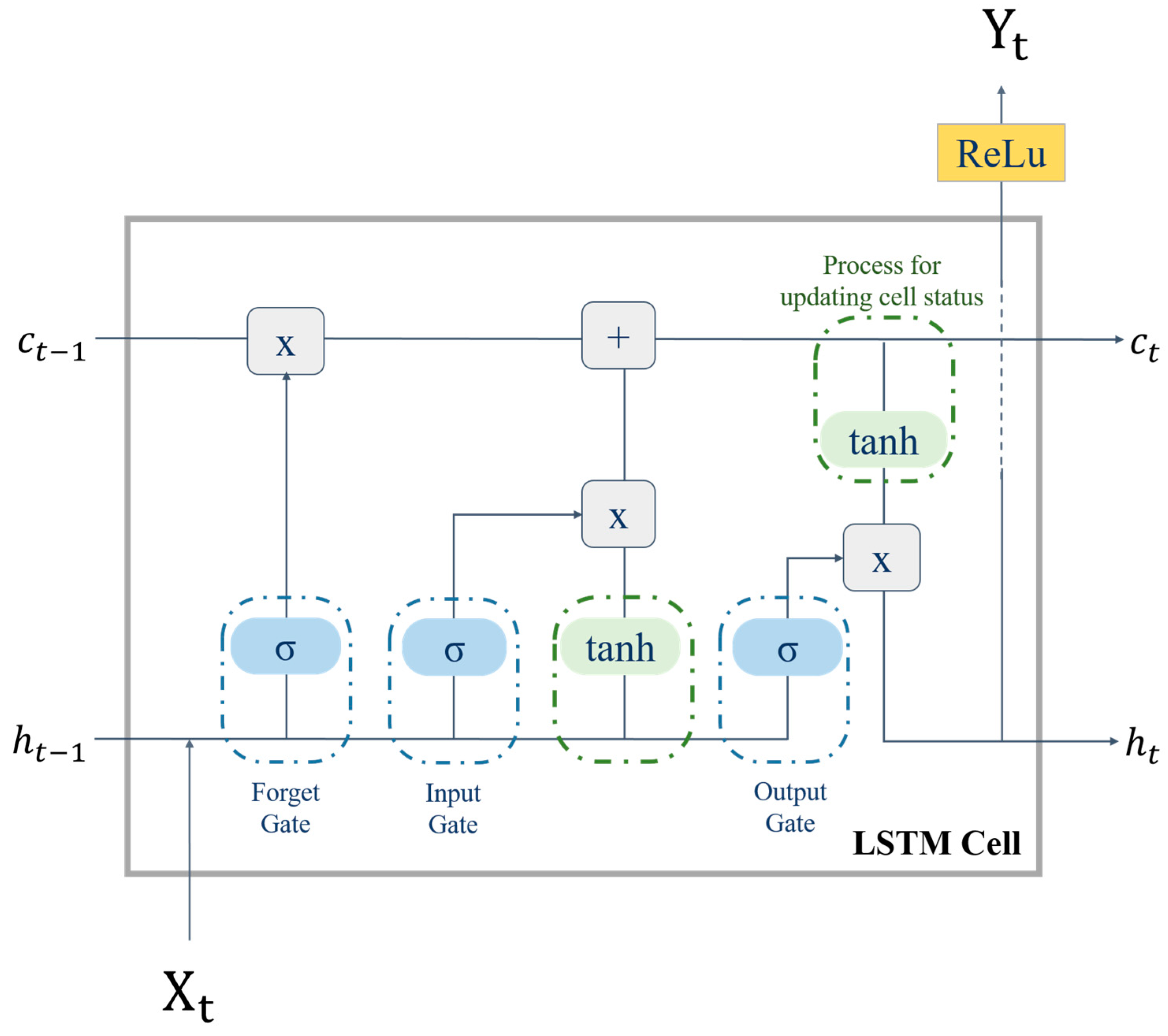
The LSTM network is a type of recurrent neural network (RNN) and was originally introduced by Hochreiter and Schmidhuber [33]. It is particularly well-suited for processing data sequences that involve long-term dependencies [34]. In contrast to a conventional RNN, which typically features a single layer of repeating modules, an LSTM network is designed with a more intricate structure that comprises four interacting layers. This sophisticated architecture serves to mitigate the issue of information loss over time and equips the network with the capability to both retain and update its internal memory states. As a result, LSTM networks excel at handling sequences with varying time intervals between significant events, making them a valuable tool in various applications involving sequential data. Figure 2 shows the structure of the LSTM neural network employed in this research.
An LSTM network comprises cell and hidden states. The cell state ( C t ) represents the memory of the LSTM unit cell, which can store propagated information over long time sequences. A candidate cell ( C t ) state is used for updating the cell state. The output of the LSTM unit cell is called the hidden state, which can carry information propagated to the next time step and is used for predictions. The hidden state ( h t ) has three gates: forget, input, and output. At time t, each gate and state can be expressed as in Equations (1)–(6). The forget gate ( f t ) determines whether information from the previous cell state should be forgotten. The input gate ( i t ) determines whether to save the current input in the cell state, and the output gate ( o t ) controls the exposure to the output.
f t = σ W x f · x t + W x f · h t 1 + b f ,
i t = σ W x i · x t + W x i · h t 1 + b i ,
o t = σ W x o · x t + W x o · h t 1 + b o ,
C t = t a n h W x c · x t + W x c · h t 1 + b c ,
C t = f t · C t 1 + i t · C t ,
h t = o t · t a n h C t ,
where x t is the input at time step t, h t 1 is the hidden state at the previous time step, W represents the weight matrices, b represents the bias factor of each gate, and σ is the sigmoid activation function.
In this study, the LSTM model was harnessed using a mini-batch training methodology, where a batch size of 64 was deliberately chosen due to its established effectiveness for flow rate prediction [35]. To safeguard against overfitting, the model underwent a total of 1000 epochs, benefiting from the inclusion of an early stopping mechanism in the Keras API. This mechanism intelligently halted the training process at the onset of any increase in validation loss. In the pursuit of optimal weight and bias adjustments, the model was equipped with the highly regarded Adam optimizer, which is acknowledged for its superior performance relative to alternative optimization algorithms [36]. The mean squared error was used as the core loss function, whereas the final model layer was enhanced with a rectified linear unit activation function.

3.2. Training Data Settings and Predictive Accuracy Assessment Method

3.2.1. Training Data Settings

In this study, nonlinear data were used in addition to existing hydrological data; therefore, it was necessary to select the optimal combination of input data. To maximize the lead time for predictions of sudden flooding, a method for reducing the number of calculations using minimal input data should be adopted. To select the optimal combination of input data, experiments were performed with different input data compositions, as listed in Table 4. Cases 1, 2, and 3 were cases without social media data. Cases 1, 2, and 4 were datasets that included only rainfall data, model simulation outflow values for owned areas, and social media data, respectively. Cases 3, 5, and 6 were datasets comprising precipitation and simulated runoff data, precipitation and social media data, and simulated runoff values and social media data, respectively. Case 7 comprised all data types. For the training periods, flooding events that occurred from April to August 2018 were used. For the testing periods used in validation, data from flooding events that occurred in September and October 2018 were employed.

3.2.2. Predictive Accuracy Assessment Method

The NSE metric was used to identify the fit of the runoff patterns of the LSTM model using various dataset compositions with crowdsourced data. This metric compares the predictive power of a model against the mean observed value and serves as a measure of the accuracy of the model predictions with the observed data. The CC values were calculated using Equation (7). The NSE is a widely used metric in hydrological modeling and other fields, where predictive accuracy assessment is important [37].
N S E = 1 t = 1 T Q o t Q m t 2 t = 1 T Q o t Q o ¯ 2 ,
where Q o t represents the observed flow rate at time t, Q m t represents the flow rate predicted from the model simulation at time t, and Q o ¯ represents the mean observed flow rate. NSE values range from infinity to 1. The closer the error variance of the estimated value to 0, the closer the NSE to 1. A value of 1 indicates a perfect match between the predicted and observed values.
The Pearson correlation coefficient (r), an efficient metric for quantifying linear distance, is a statistical measure that is widely used to understand the degree of linear trend between two variables [38]. Equation (8) shows the formula for r. r ranges from −1 to 1, where −1 indicates a perfect negative correlation, 1 indicates a perfect positive correlation, and 0 indicates no linear correlation.
= i = 1 n ( x i x ¯ ) ( y i y ¯ ) i = 0 n ( x i x ¯ ) 2 i = 0 n ( y i y ¯ ) 2 ,
where the numerator ( i = 1 n ( x i x ¯ ) ( y i y ¯ ) ) represents the variances of x and y , and the denominator ( i = 0 n ( x i x ¯ ) 2 i = 0 n ( y i y ¯ ) 2 ) represents the variances of each x and y .
The normalized root mean square error (NRMSE) was also used to evaluate the model accuracy. The NRMSE quantifies the difference between the observed and predicted values at different scales. In this study, the NRMSE between the observed and predicted data values was calculated to examine quantitative differences and easily compare accuracy. The NRMSE is expressed as in Equation (9).
N R M S E % = i = 1 n y i y ^ i 2 n y m a x y m i n × 100 ,
where y i and y ^ i are the observed and predicted values from the model, respectively, and ( y i y ^ i ) 2 indicates the squared difference between two data points.

4. Experiment Results

As lead time is important in the case of sudden flooding, the outflow of the Jungnang stream was predicted at 30 min, 1 h, 2 h, and 3 h before the flood event for Cases 1–7, and the results were compared. Figure 3 summarizes the prediction results for each case. Contrary to the belief that the shorter the lead time, the higher the accuracy, the accuracy was higher for a lead time of 1 h than for 30 min in all cases.
Cases 1 and 5, 2 and 6, and 3 and 7 were compared to evaluate whether social media data contributed to the model’s predictive power. The results showed that the NSE and r values increased, and the NRMSE decreased, indicating more accurate predictions. In particular, in Case 1 and Case 4, which were predicted using only rainfall data and social media data, respectively, the r was low, and the NSE was negative. In Case 1, rainfall data from the point located upstream were used; therefore, it is likely that there was a limit to predicting the flow rate of the entire watershed. The outcome in Case 4 can be attributed to the time lag between the occurrence of rainfall and flow rate changes and the subsequent generation of social media content. Thus, this outcome leads to the conclusion that relying solely on social media data has its limitations. In the prediction with a 60 min lead time for Case 5, the accuracy was lower than for the other datasets for the same reason. However, comparing the overall indicator change, the NSE increased by approximately 77% from 0.35 to 0.62, and r increased by 0.07 from 0.76 to 0.83, demonstrating a 9% increase. The NRMSE also decreased by 0.27, corresponding to a 14% reduction. This was similar for Cases 2, 6, 3, and 7.
Cases 2, 3, 6, and 7 exhibited high accuracy in modeling the outflows. Figure 3 compares the observed values of Cases 2, 3, 6, and 7, indicating high accuracy with the prediction values obtained through the model. The 60 min prediction for Case 2 showed an NSE of 0.89, r of 0.95, and NRMSE of 1.16%. However, the accuracy indicators NSE, r, and r2 increased in Cases 3 and 6 compared with those in Case 2. The 30 min lead time prediction results in Cases 2 and 3 were similar; for other lead times, they showed better results than when modeling values alone were used. The 30 min and 1 h predictions were more accurate with the combination of social media and model values than with the combination of rainfall and model values. The 2 h and 3 h predictions were more accurate with combinations of rainfall and model values. Reflecting the outflow was expected to take time as rainfall data were used as an input. Case 7 was the most accurate. Unlike other cases, where achieving 80% accuracy was challenging, Case 7 yielded an NSE of 0.82 and r of 0.91 for the 2 h prediction.
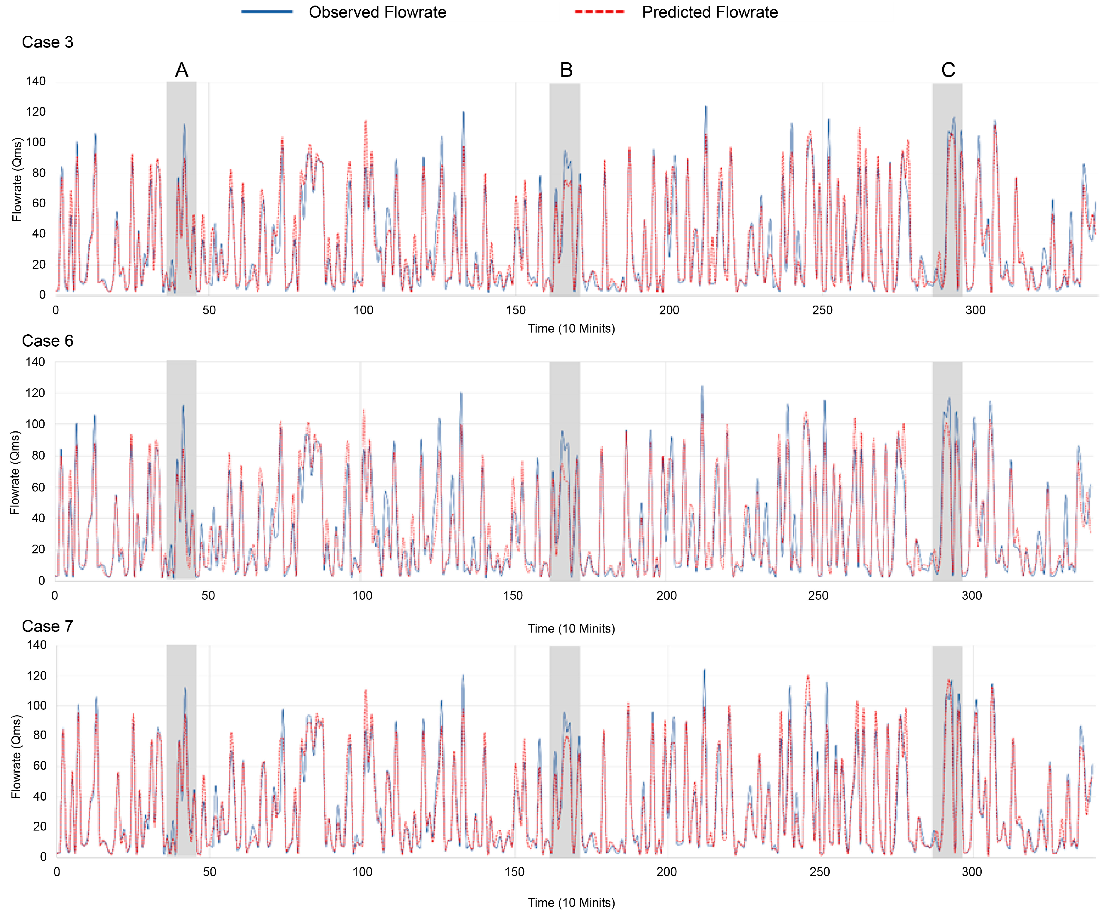
As above-mentioned, Case 7, in which all data were included as input factors, was the most accurate. Case 4, which used only social media data, had the lowest accuracy. The results confirmed that social media data helped improve prediction accuracy; however, the bias was large when social media was the only input factor. In addition, in the graphs for Case 2 (Figure 4), which used only the modeling flow values for the prediction, the loop shape was less visible in the 30 min and 1 h lead-time predictions but clear in the 2 h and 3 h predictions. This result was expected from the time-series prediction with a time delay. The loop shape disappeared when social media data were included as an input factor (Cases 6 and 7). The time-series prediction results were compared to determine the peak flow rate consistency and occurrence time, which are the most significant factors in predicting sudden flooding. Figure 5 compares the predicted and observed values for Cases 3, 6, and 7.
The peak flow rate and its time of occurrence are vital to flood forecasting. Case 7 more accurately predicted the peak flow rate than Cases 3 and 6. This was particularly evident in Section A, where two peak flow generation intervals of 60 Qms or more were observed. In Case 3, a flow rate of approximately 80 Qms was adjusted relatively accurately; however, the result was predicted at 90 Qms at an observed flow rate of 110 Qms. This result was similar to that of Case 6. Case 7 accurately matched 80 Qms and showed better results than the previous combination, although it was less than 110 Qms at the second peak. This was similar to the results of Case 3, which used the rainfall and model flow values and implemented the shapes of the two peaks similarly; however, the difference in the peak flow was large. In Case 7, the shape of the peak was not implemented, but the result was most similar to the peak flow rate. The difference in the flow rate was predicted the least in Section C. These results indicate that social media data influence prediction accuracy; however, the peak flow rate can be more accurately predicted only when rainfall, social media, and modeling flow values are used together.

5. Discussion

Accurate flood prediction is of paramount importance for enabling swift evacuation measures and effective road control, ultimately mitigating the risks associated with flood-related human harm and property damage. Nevertheless, attaining precision in rapid response to flash floods remains a formidable challenge, particularly in ungauged basins lacking hydrological data. This study introduced an innovative approach by harnessing unstructured social media data in conjunction with an LSTM network model to predict flood events. The study also assessed the feasibility of utilizing social media as an alternative data source to hydrological input for ungauged basins. The findings underscore the enhanced accuracy achieved through the incorporation of social media data, revealing its substantial predictive potential when integrated with other input variables.
This study’s results corroborate those of Songchon et al., who pointed out that uncertainty in flood forecasting models can be reduced by employing social media data [29]. Abas and Addou also indicated that social media is a considerable variable in predicting flooding on a map [29]. In addition, it has been demonstrated that social media records can be used to improve local flood forecasting by storing the conditions in a database [39]. Although the accuracy of the discharge predictions in the present study was slightly lower than in prior studies [14,15,16], a commendable level of over 90% accuracy in terms of the NSE was maintained. Given the prevalent reliance on similar methodologies for hourly unit forecasts, models achieving an NSE of 0.94 and a correlation coefficient of 0.97 are deemed appropriate when focusing on 10 min predictions to ensure accuracy during flash flood occurrences.
This study has several limitations that present opportunities for future research. First, social media may contain inaccurate information or exhibit biases because they rely on data generated by humans. Therefore, solely assessing the quantity of data may not provide a precise gauge of the severity of a flood. Furthermore, many researchers have conducted studies on flood detection and estimation using social media images in addition to text data [40,41,42,43,44,45,46,47] since photos and videos can serve as crucial indicators of real-time field conditions [43]. The authors of the present study intend to incorporate additional image data analysis and sentiment analysis of textual data into future research to enhance the predictive accuracy of flood assessment. Second, this study only employed an LSTM model, which focused on identifying the optimal combination of input variables; however, it is imperative to analyze alternative models. Furthermore, developing a novel model for optimizing various combinations is necessary while considering the creation of previously unused input factors.

6. Conclusions

This study proposed optimized input variables to enhance flood prediction accuracy for ungauged basins, i.e., basins that lack hydrological data, using an LSTM network model and social media data as an alternative to observation data. Several cases were divided by different combinations of crowdsourced data and existing hydrological elements to find the optimal dataset for prediction. An analysis of the influence of social media data on the model’s predictive power revealed significant improvements in accuracy, as indicated by metrics such as the NSE and r values, and a reduction in the NRMSE. The main findings of this study can be summarized as follows.
(1)
In general, the model’s prediction accuracy improved when social media data were used as an input factor along with other factors.
(2)
The study found that combinations of social media and modeling data yielded better accuracy for 1 h predictions, whereas combinations of rainfall and modeling data provided more accuracy in the 30 min, 2 h, and 3 h predictions.
(3)
Notably, cases that included all data as input factors demonstrated the highest accuracy, achieving an NSE of 82 and r of 0.91 in the 2 h predictions.
The study demonstrated that using social media as an alternative data source in LSTM models has the potential to enhance flood prediction accuracy in regions with limited data availability. Future studies should focus on constructing a neural network model that can improve the accuracy of the optimal input factors identified in this study. Moreover, research on predicting the severity of flooding by configuring the results of sentence analyses of social media text data, with words as input factors, is necessary.

Author Contributions

Conceptualization, J.L. and S.H.; methodology, J.L.; coding, J.L.; writing—original draft preparation, J.L. and S.H.; writing—review and editing, J.L. and S.H.; visualization, J.L.; supervision, S.H. All authors have read and agreed to the published version of the manuscript.

Funding

This research was supported by the National Research Foundation of Korea Grant funded by the Korean government (Ministry of Science and ICT), grant number NRF-2020R1A2C2014937.

Data Availability Statement

Not applicable.

Conflicts of Interest

The authors declare no conflict of interest.

References

  1. World Meteorological Organization. State of the Global Climate; WMO: Geneva, Switzerland, 2022. [Google Scholar]
  2. Shkolnik, I.; Pavlova, T.; Efimov, S.; Zhuravlev, S. Future changes in peak river flows across northern Eurasia as inferred from an ensemble of regional climate projections under the IPCC RCP8. 5 scenario. Clim. Dyn. 2018, 50, 215–230. [Google Scholar] [CrossRef]
  3. Zhou, Q.; Leng, G.; Su, J.; Ren, Y. Comparison of urbanization and climate change impacts on urban flood volumes: Importance of urban planning and drainage adaptation. Sci. Total Environ. 2019, 658, 24–33. [Google Scholar] [CrossRef] [PubMed]
  4. Dhunny, A.Z.; Seebocus, R.H.; Allam, Z.; Chuttur, M.Y.; Eltahan, M.; Mehta, H. Flood prediction using artificial neural networks: Empirical evidence from Mauritius as a case study. Knowl. Eng. Data Sci. 2020, 3, 1–10. [Google Scholar] [CrossRef]
  5. Duncan, A.; Chen, A.S.; Keedwell, E.; Djordjevic, S.; Savic, D. Urban flood prediction in real-time from weather radar and rainfall data using artificial neural networks. In Proceedings of the Weather Radar and Hydrology: IAHS Red Book Proceedings, Exeter, UK, 18–21 April 2011. [Google Scholar]
  6. Lee, J.; Hwang, S. Water level prediction of small and medium-sized rivers using artificial neural networks. J. Korean Soc. Hazard Mitig. 2022, 22, 61–68. [Google Scholar] [CrossRef]
  7. Rezaeianzadeh, M.; Tabari, H.; Arabi Yazdi, A.; Isik, S.; Kalin, L. Flood flow forecasting using ANN, ANFIS and regression models. Neural Comput. Appl. 2014, 25, 25–37. [Google Scholar] [CrossRef]
  8. Samantaray, S.; Agnihotri, A.; Sahoo, A. Flood Replication Using ANN Model Concerning with Various Catchment Characteristics: Narmada River Basin. J. Inst. Eng. (India) A 2023, 104, 381–396. [Google Scholar] [CrossRef]
  9. Shrestha, R.R.; Theobald, S.; Nestmann, F. Simulation of flood flow in a river system using artificial neural networks. Hydrol. Earth Syst. Sci. 2005, 9, 313–321. [Google Scholar] [CrossRef]
  10. Tawfik, A.M. River flood routing using artificial neural networks. Ain Shams Eng. J. 2023, 14, 101904. [Google Scholar] [CrossRef]
  11. Tsakiri, K.; Marsellos, A.; Kapetanakis, S. Artificial neural network and multiple linear regression for flood prediction in Mohawk River, New York. Water 2018, 10, 1158. [Google Scholar] [CrossRef]
  12. Mirzaei, S.; Vafakhah, M.; Pradhan, B.; Alavi, S.J. Flood susceptibility assessment using extreme gradient boosting (EGB), Iran. Earth Sci. Inform. 2021, 14, 51–67. [Google Scholar] [CrossRef]
  13. Ilhan, A. Forecasting of river water flow rate with machine learning. Neural Comput. Appl. 2022, 34, 20341–20363. [Google Scholar] [CrossRef]
  14. Le, X.H.; Nguyen, D.H.; Jung, S.; Yeon, M.; Lee, G. Comparison of deep learning techniques for river streamflow forecasting. IEEE Access 2021, 9, 71805–71820. [Google Scholar] [CrossRef]
  15. Dehghani, A.; Moazam, H.M.Z.H.; Mortazavizadeh, F.; Ranjbar, V.; Mirzaei, M.; Mortezavi, S.; Ng, J.L.; Dehghani, A. Comparative evaluation of LSTM, CNN, and ConvLSTM for hourly short-term streamflow forecasting using deep learning approaches. Ecol. Inform. 2023, 75, 102119. [Google Scholar] [CrossRef]
  16. Atashi, V.; Kardan, R.; Gorji, H.T.; Lim, Y.H. Comparative Study of Deep Learning LSTM and 1D-CNN Models for Real-time Flood Prediction in Red River of the North, USA. In Proceedings of the 2023 IEEE International Conference on Electro Information Technology (eIT), Romeoville, IL, USA, 18–20 May 2023; pp. 22–28. [Google Scholar] [CrossRef]
  17. Guo, Y.; Zhang, Y.; Zhang, L.; Wang, Z. Regionalization of hydrological modeling for predicting streamflow in ungauged catchments: A comprehensive review. WIREs Water 2021, 8, e1487. [Google Scholar] [CrossRef]
  18. Kastridis, A.; Kirkenidis, C.; Sapountzis, M. An integrated approach of flash flood analysis in ungauged Mediterranean watersheds using post-flood surveys and unmanned aerial vehicles. Hydrol. Process. 2020, 34, 4920–4939. [Google Scholar] [CrossRef]
  19. Liu, L. Unravelling and improving the potential of global discharge reanalysis dataset in streamflow estimation in ungauged basins. J. Clean. Prod. 2023, 419, 138282. [Google Scholar] [CrossRef]
  20. Xiao, Q.; Zhou, L.; Xiang, X.; Liu, L.; Liu, X.; Li, X.; Ao, T. Integration of Hydrological Model and Time Series Model for Improving the Runoff Simulation: A Case Study on BTOP Model in Zhou River Basin, China. Appl. Sci. 2022, 12, 6883. [Google Scholar] [CrossRef]
  21. Zhu, Y.; Liu, L.; Qin, F.; Zhou, L.; Zhang, X.; Chen, T.; Li, X.; Ao, T. Application of the regression-augmented regionalization approach for BTOP model in ungauged basins. Water 2021, 13, 2294. [Google Scholar] [CrossRef]
  22. Kheimi, M.; Almadani, M.; Zounemat-Kermani, M. Stochastic (S [ARIMA]), shallow (NARnet, NAR-GMDH, OS-ELM), and deep learning (LSTM, Stacked-LSTM, CNN-GRU) models, application to river flow forecasting. Acta Geophys. 2023, 1–15, 82. [Google Scholar] [CrossRef]
  23. Fohringer, J.; Dransch, D.; Kreibich, H.; Schröter, K.J. Social media as an information source for rapid flood inundation mapping. Nat. Hazards Earth Syst. Sci. 2015, 15, 2725–2738. [Google Scholar] [CrossRef]
  24. Herfort, B.; De Albuquerque, J.P.; Schelhorn, S.J.; Zipf, A.B. Exploring the geographical relations between social media and flood phenomena to improve situational awareness. In Connecting a Digital Europe through Location and Place; Huerta, J., Schade, S., Granell, C., Eds.; Springer: Castellon, Spain, 2014; pp. 55–71. [Google Scholar] [CrossRef]
  25. Lee, J.; Hwang, S.J. A study on the application of social network service data for monitoring flood damage. J. Korean Soc. Hazard Mitig. 2019, 19, 77–85. [Google Scholar] [CrossRef]
  26. Murthy, D.; Longwell, S.A.D. Twitter and disasters: The uses of Twitter during the 2010 Pakistan floods. Inf. Commun. Soc. 2013, 16, 837–855. [Google Scholar] [CrossRef]
  27. Spielhofer, T.; Greenlaw, R.; Markham, D.; Hahne, A. Data mining Twitter during the UK floods: Investigating the potential use of social media in emergency management. In Proceedings of the 2016 3rd International Conference on Information and Communication Technologies for Disaster Management (ICT-DM), Vienna, Austria, 13–15 December 2016; pp. 1–6. [Google Scholar] [CrossRef]
  28. Kanth, A.K.; Chitra, P.; Sowmya, G.G. Deep learning-based assessment of flood severity using social media streams. Stoch. Environ. Res. Risk Assess. 2022, 36, 473–493. [Google Scholar] [CrossRef]
  29. Songchon, C.; Wright, G.; Beevers, L. The use of crowdsourced social media data to improve flood forecasting. J. Hydrol. 2023, 622, 129703. [Google Scholar] [CrossRef]
  30. Jungnangcheon Area (Seoul Metropolitan Government) River Basic Plan; Ministry of Land, Transport and Maritime Affairs: Sejong, Republic of Korea, 2012.
  31. Jungnangcheon Area (Gyeonggi-Dogovernment) River Basic Plan; Ministry of Land, Transport and Maritime Affairs: Sejong, Republic of Korea, 2012.
  32. Corps of Engineers Washington DC. Flood-Runoff Analysis; US Army Corps of Engineers: Washington, DC, USA, 1994.
  33. Hochreiter, S.; Schmidhuber, J. Long short-term memory. Neural Comput. 1997, 9, 1735–1780. [Google Scholar] [CrossRef] [PubMed]
  34. Gers, F.A.; Schmidhuber, J.; Cummins, F. Learning to forget: Continual prediction with LSTM. Neural Comput. 2000, 12, 2451–2471. [Google Scholar] [CrossRef]
  35. Xiang, Z.; Yan, J.; Demir, I. A rainfall-runoff model with LSTM-based sequence-to-sequence learning. Water Resour. Res. 2020, 56, e2019WR025326. [Google Scholar] [CrossRef]
  36. Kingma, D.P.; Ba, J. Adam: A method for stochastic optimization. arXiv 2014, arXiv:1412.6980. [Google Scholar] [CrossRef]
  37. Gupta, H.V.; Kling, H.; Yilmaz, K.K.; Martinez, G.F. Decomposition of the mean squared error and NSE performance criteria: Implications for improving hydrological modelling. J. Hydrol. 2009, 377, 80–91. [Google Scholar] [CrossRef]
  38. Chen, R.; Ju, M.; Chu, C.; Jing, W.; Wang, Y. Identification and quantification of physicochemical parameters influencing chlorophyll-a concentrations through combined principal component analysis and factor analysis: A case study of the Yuqiao Reservoir in China. Sustainability 2018, 10, 936. [Google Scholar] [CrossRef]
  39. Abas, S.; Addou, M. Geospatial Forecasting and Social Media Exploration Based on Sentiment Analysis: Application to Flood Forecasting. Geospat. Intell. Appl. Future Trends 2022, 19–29. [Google Scholar]
  40. Brown, J.M.; Yelland, M.J.; Pullen, T.; Silva, E.; Martin, A.; Gold, I.; Whittle, L.; Wisse, P. Novel use of social media to assess and improve coastal flood forecasts and hazard alerts. Sci. Rep. 2021, 11, 13727. [Google Scholar] [CrossRef] [PubMed]
  41. Eilander, D.; Trambauer, P.; Wagemaker, J.; Van Loenen, A. Harvesting social media for generation of near real-time flood maps. Procedia Eng. 2016, 154, 176–183. [Google Scholar] [CrossRef]
  42. Li, Y.; Osei, F.B.; Hu, T.; Stein, A. Urban flood susceptibility mapping based on social media data in Chengdu city, China. Sustain. Cities Soc. 2023, 88, 104307. [Google Scholar] [CrossRef]
  43. Yang, T.; Xie, J.; Li, G.; Zhang, L.; Mou, N.; Wang, H.; Zhang, X.; Wang, X. Extracting disaster-related location information through social media to assist remote sensing for disaster analysis: The case of the flood disaster in the Yangtze River Basin in China in 2020. Remote Sens. 2022, 14, 1199. [Google Scholar] [CrossRef]
  44. Chaudhary, P.; D’Aronco, S.; Moy de Vitry, M.; Leitão, J.P.; Wegner, J.D. Flood-water level estimation from social media images. ISPRS Ann. Photogram. Remote Sens. Spat. Inf. Sci. 2019, 4, 5–12. [Google Scholar] [CrossRef]
  45. Rosser, J.F.; Leibovici, D.G.; Jackson, M.J. Rapid flood inundation mapping using social media, remote sensing and topographic data. Nat. Hazards 2017, 87, 103–120. [Google Scholar] [CrossRef]
  46. Smith, L.; Liang, Q.; James, P.; Lin, W. Assessing the utility of social media as a data source for flood risk management using a real-time modelling framework. J. Flood Risk Manag. 2017, 10, 370–380. [Google Scholar] [CrossRef]
  47. Asif, A.; Khatoon, S.; Hasan, M.M.; Alshamari, M.A.; Abdou, S.; Elsayed, K.M.; Rashwan, M. Automatic analysis of social media images to identify disaster type and infer appropriate emergency response. J. Big Data 2021, 8, 83. [Google Scholar] [CrossRef]
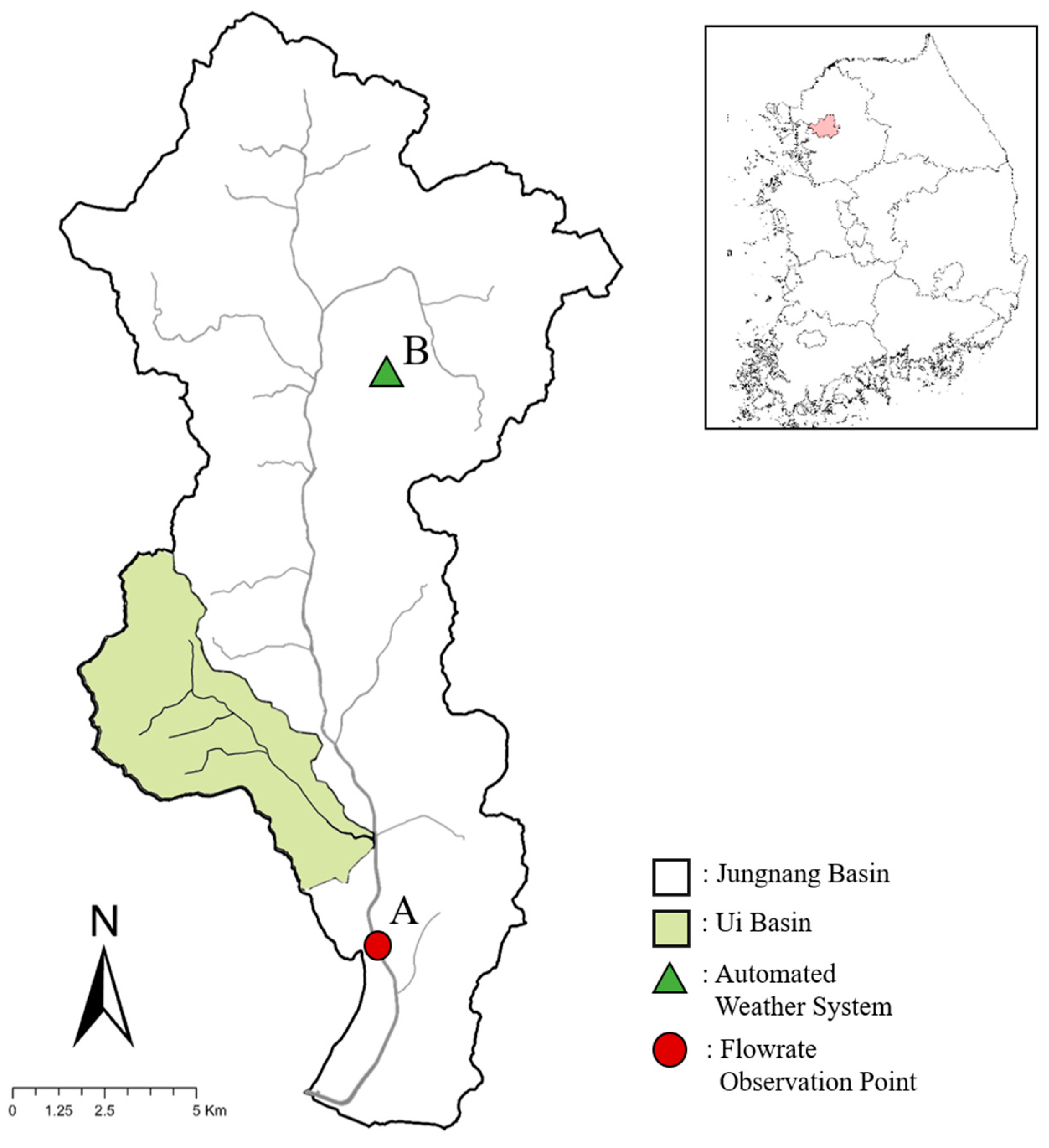
Figure 1. Location of the Jungnang Basin and Ui Basin.
Water 15 03818 g001
Figure 2. Structure of the LSTM model used in this study.
Water 15 03818 g002
Figure 3. Flow rate prediction results: (a) 30 min prediction, (b) 60 min prediction, (c) 120 min prediction, (d) 180 min prediction.
Water 15 03818 g003
Figure 4. Comparison of prediction results between cases, including modeling flow rate.
Water 15 03818 g004
Figure 5. Comparison between observed and predicted flow rates (Cases 3, 6, and 7) and three peak points with different predictive power (A, B, and C).
Water 15 03818 g005
Table 1. Observation data used in the study.
DataUnit
(Total
Data Count)
UsageLocationSource
Precipitation10 min
(2448)
Input VariableUpstream of Jungnang Basin (B)Korea Meteorological Administration
Flow rateOutput VariableDownstream of Jungnang Basin (A)Han River Flood Control Office
Table 2. Routing methods and parameters used in the Hec-1 model.
Routing MethodParametersFormula
CLARK watershed
routing method
Travel Time (TC)Kraven (II) [30]
Storage Constant (R)Sabol formula [32]
Muskingum hydrologic channel flood routing methodRetention Constant (K)Passage time of the peak flood from the HEC-RAS unsteady flow model
Table 3. Variables included in the social media data content.
VariableDescription
KeywordConfiguring disaster types with keywords
RegionExtracting local information where the event occurred
TimeEnabled a specified search of the time when the event occurred and extracted the time when the social media post was created
TitleExtracted to determine if the content contained in the body of the social media post was relevant to local information or crisis events
Article
Web addressPrevented data from being stored when data from the same address was extracted to avoid duplicate data
Meteorological dataExtracted for comparative analysis with weather-related disasters
Table 4. Composition of each input dataset.
Dataset Case No.Training PeriodsTesting PeriodsInput Data Composition
PrecipitationFlow Rate
(Model)
Social Media
122–24 April 2018
16–18 May 2018
26–28 June 2018
1–3 July 2018
26–28 August 2018
3–5 September 2018
6–8 October 2018
2
3
4
5
6
7
Disclaimer/Publisher’s Note: The statements, opinions and data contained in all publications are solely those of the individual author(s) and contributor(s) and not of MDPI and/or the editor(s). MDPI and/or the editor(s) disclaim responsibility for any injury to people or property resulting from any ideas, methods, instructions or products referred to in the content.