Peaks-Over-Threshold-Based Regional Flood Frequency Analysis Using Regularised Linear Models

Abstract

Regional flood frequency analysis (RFFA) is widely used to estimate design floods in ungauged catchments. Most of the RFFA techniques are based on the annual maximum (AM) flood model; however, research has shown that the peaks-over-threshold (POT) model has greater flexibility than the AM model. There is a lack of studies on POT-based RFFA techniques. This paper presents the development of POT-based RFFA techniques, using regularised linear models (least absolute shrinkage and selection operator, ridge regression and elastic net regression). The results of these regularised linear models are compared with multiple linear regression. Data from 145 stream gauging stations of south-east Australia are used in this study. A leave-one-out cross-validation is adopted to compare these regression models. It has been found that the regularised linear models provide quite accurate flood quantile estimates, with a median relative error in the range of 37 to 47%, which outperform the AM-based RFFA techniques currently recommended in the Australian Rainfall and Runoff guideline. The developed RFFA technique can be used to estimate flood quantiles in ungauged catchments in the study region.

1. Introduction

Floods rank among the most severe natural disasters, resulting in substantial economic losses and tragic loss of human life on an annual basis. Between 1980 and 2016, flood-related incidents caused more than 240,000 deaths and caused damages amounting to almost USD 1 trillion [1]. The economic impact of floods in Australia is considerable, with the average annual flood damage amounting to more than AUD 377 million and infrastructure that necessitates design flood estimates valued at over AUD 1 billion per year. The New South Wales and south-east Queensland floods of February and March 2022 alone accounted for AUD 5.65 billion. This highlights the need for more accurate and reliable design flood estimation methods, which can reduce the overall flood damage.

Flood frequency analysis is a critical component of flood risk assessment and management, providing estimates of the frequency and magnitude of extreme flood events that are crucial for designing infrastructure and making decisions related to flood risk. Traditionally, flood frequency analysis has been based on the assumption that the flood data follow a particular distribution (e.g., the Gumbel distribution) [2], which is then used to estimate flood quantiles. However, this approach can be limiting, as it assumes a fixed distribution that may not accurately capture the underlying flood characteristics, particularly for extreme events [3,4]. To conduct flood frequency analysis, the two main models, the annual maximum (AM) and the peaks-over-threshold (POT), are generally adopted [5,6,7]. The AM model involves fitting a statistical distribution to the AM flood data. This method assumes that the largest flood in each year is representative of the maximum flood potential for that year. While the AM method is simple and widely used, it considers many smaller flood data points from relatively dry years and ignores some large data points from wet years [8]. The POT approach offers a more flexible and efficient way to estimate the tails of the flood frequency distribution by modelling the exceedances over a site-specific threshold level [9].

Regional flood frequency analysis (RFFA) is a widely used approach to estimate flood quantiles in ungauged catchments. It involves two steps: forming regions based on similarities in hydrological characteristics and applying statistical techniques (such as the index flood method or quantile regression technique) for design flood estimation. RFFA enables transferring flood characteristics from gauged to ungauged sites within the same region, providing a systematic means of estimating flood quantiles at any arbitrary location within the region. AM-flood-based RFFA is widely adopted internationally, providing a straightforward practice, and only limited research has focused on POT-based RFFA. Recently, Pan et al. [10] developed a POT-based RFFA technique for south-east Australia and found that ordinary least squares (OLS) performs better than the weighted-least-squares (WLS)-based regression techniques.

While the POT-based RFFA method has shown great promise in estimating flood quantiles at ungauged catchments, it can suffer from overfitting and poor generalisation performance, with a large number of predictors or highly correlated predictors [11]. To overcome these challenges, regularised linear models, such as least absolute shrinkage and selection operator (LASSO) [12], ridge regression (RR) [13] and elastic net regression (EN) [14] have been proposed as effective solutions. These models introduce a penalty term to the loss function, which helps to avoid overfitting and to produce more stable and reliable estimates of the regression coefficients. However, the performance of different regularised linear models within the POT framework in RFFA has not been fully explored.

Table 1. Results of search queries in different databases.

Search Query with Boolean Operators	Number of Documents
	Scopus (Title, Abstract, Keyword)	Dimensions (Title and Abstract)	Web of Science (Topic 1)
“Peaks over threshold”	1394	1332	695
“Partial duration series”	301	251	291
(“Partial duration series” OR “peaks over threshold”)	1673	1563	954
(“Partial duration series” OR “peaks over threshold”) AND (flood)	437	384	307
(“Partial duration series” OR “peaks over threshold”) AND (flood) AND (“Multiple Linear Regression” OR “Least Absolute Shrinkage and Selection Operator” OR LASSO OR “Ridge Regression” OR “Elastic Net Regression”)	3	1	2

Note: ¹ Searches title, abstract, author keywords and Keywords Plus.

presents number of studies published which have used the POT model in flood research with at least one of the regularised linear models (LASSO, RR or EN).

Scopus has captured three articles [15,16,17] which meet the search criteria, whereas Dimensions and Web of Science have found one [16] and two [15,16] published articles, respectively. When we dive deep into these three articles, it is evident that none of them fully meet the defined search criteria. The reason is that these three articles are selected based on the keywords, titles and abstracts in the articles, to which the search query was restricted; however, they did not apply any of the regularised linear models within POT-based RFFA.

This study aims to fill the current knowledge gap by comparing the performance of different regularised linear models within the POT framework in RFFA. Specifically, we focus on the ability of LASSO, RR and EN to accurately estimate design floods in ungauged catchments. We evaluate these regularised linear models using flood and catchment characteristics data from south-east Australia, based on a leave-one-out cross-validation (LOOCV) technique.

2. Materials and Methods

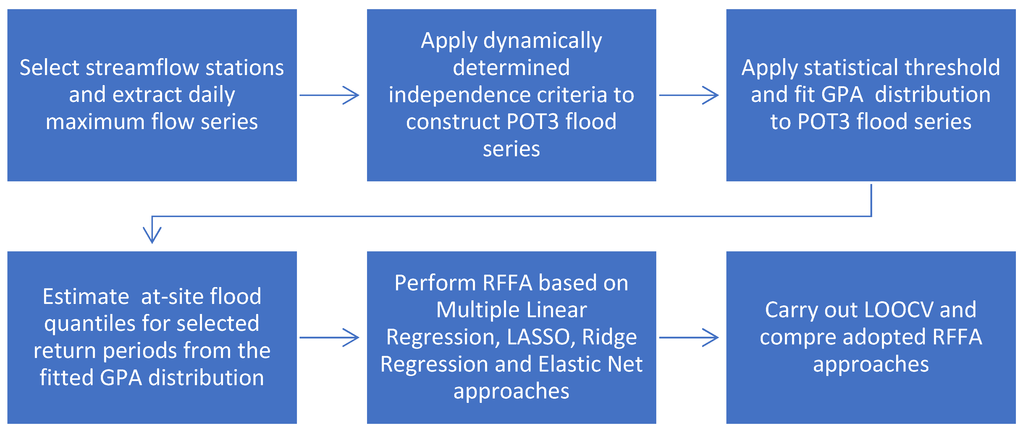
The study involves several steps, as illustrated in Figure 1. Initially, study area and catchments were selected. For each of the selected catchments, POT flow series was extracted and flood quantiles were estimated. A catchment characteristics data set was extracted for each of the catchments. For the selected flood quantiles, prediction equations were developed by multiple linear regression and penalised regression analyses. A leave-one-out cross validation (LOOCV) approach was adopted to evaluate the performance of the developed prediction equations. R software was used to carry out the analyses [18]. These steps are described below.

2.1. Study Area and Data

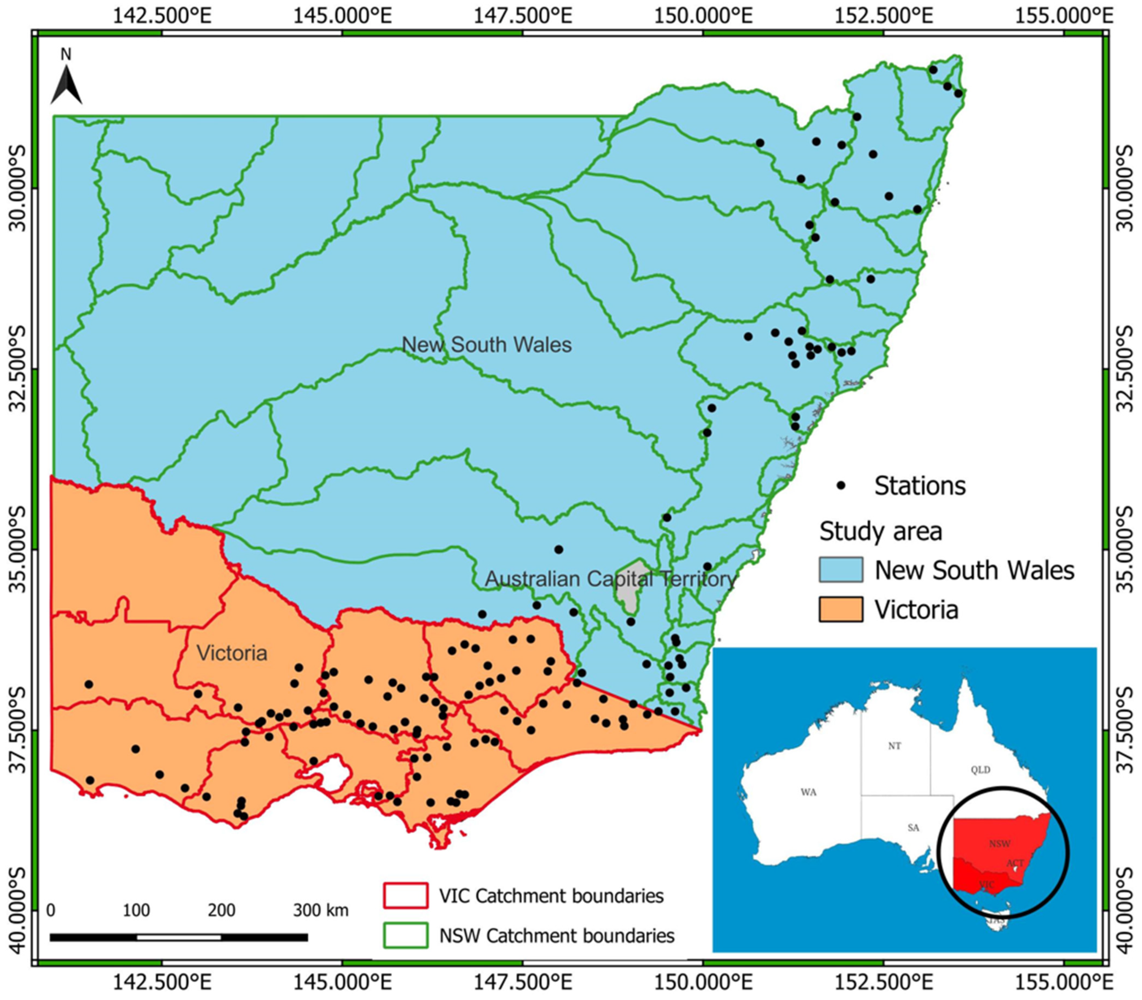
This study selects 145 stream gauging stations across the south-east region of Australia. The reason for selecting this region is the availability of high-quality streamflow data in this region compared to other parts of Australia. Figure 2 shows the geographical location of the selected stations. The catchment area of the selected stations ranges from 11 km² to 1010 km², with an average of 360 km² and a median of 310 km². Records of streamflow data range from 27 to 83 years, with an average of 42 years. Among selected stations, 55 are from New South Wales (NSW) and 90 are from Victoria (VIC), both of which are Australian states.

Application of the Hosking and Wallis [19] homogeneity test indicated that the stations do not form homogeneous regions, as H statistics values were over 10. For a region to be homogeneous, H statistics should be smaller than 1.00.

The selected stations are located on both sides of the Great Dividing Range (GDR) of Australia, which measures approximately 3500 km, starting from the state of Queensland and ending at the eastern edge of the state of Victoria. The GDR divides the coastal region of south-eastern Australia into coastal and inland plains. The rationale for including both areas is based on the previous studies of Ali and Rahman [20] and Zalnezhad et al. [21], which suggest considering both inland and coastal as a single region for RFFA.

A total of seven catchment characteristics are adopted as independent variables in this study. The adopted independent variables, which include catchment area (A, km²), mean annual rainfall (MAR, mm), catchment shape factor (SF, fraction), mean annual evapotranspiration (MAE, mm), catchment stream density (SDEN, km⁻¹), catchment mainstream slope (S1085, m·km⁻¹) and forest (FST, fraction), are summarised in

Table 2. Descriptive statistics of the independent variables based on the selected 145 catchments in New South Wales and Victoria, Australia.

Independent Variable	Minimum	Maximum	Mean	Median	Standard Deviation
A (km2)	11.00	1010.00	360.21	310.00	258.77
MAR (mm)	485.32	1953.23	1001.80	926.96	327.85
SF (fraction)	0.26	1.43	0.77	0.77	0.21
MAE (mm)	932.70	1543.30	1111.25	1068.80	130.44
SDEN (km−1)	0.52	5.47	1.97	1.58	1.01
S1085 (m/km)	0.80	69.90	12.77	9.59	10.95
FST (fraction)	0.01	1.00	0.59	0.65	0.33

.

Table 3. Correlation coefficients (with their corresponding p-values) between the independent variables (NA means not applicable).

	A	MAR	SF	MAE	SDEN	S1085	FST
A	1.000
	NA
MAR	−0.140	1.000
	0.093	NA
SF	−0.009	−0.073	1.000
	0.914	0.383	NA
MAE	−0.080	0.346	0.038	1.000
	0.338	0.000	0.652	NA
SDEN	−0.219	0.347	0.067	0.615	1.000
	0.008	0.000	0.424	0.000	NA
S1085	−0.463	0.206	−0.004	−0.097	0.161	1.000
	0.000	0.013	0.962	0.247	0.054	NA
FST	0.015	0.328	0.048	−0.022	0.173	0.437	1.000
	0.863	0.000	0.566	0.791	0.037	0.000	NA

shows the correlation coefficients of the independent variables. It was found that some of the variables were highly correlated. However, the Durbin–Watson statistics of the developed regression equations were close to 2.00, indicating that they did not have much impact on the regression analysis. Penalised regression (as adopted here) is more capable of dealing with the highly correlated variables.

2.2. At-Site Flood Frequency Analysis

The dependent variable selected in the regression model is Q_T (flood discharge for T-year return period), which is estimated by at-site flood frequency analysis.

The initial step in any at-site flood frequency analysis is the fitting of a probability distribution to the observed flood data. The generalised Pareto (GPA) distribution, along with its reduced form, the exponential distribution, remains a widely favoured choice for flood frequency analysis based on a POT approach [22,23,24,25]. The employment of extreme value theory, as introduced by Pickands III [26], has been deemed appropriate for this purpose. Among these distributions, the two-parameter GPA distribution is preferred in POT-based flood frequency analysis over the one-parameter exponential distribution due to its enhanced modelling flexibility, and, hence, GPA was adopted in this study. Six return periods or average recurrence intervals (ARIs) are considered in this study, which are 2, 5, 10, 20, 50 and 100 years.

The at-site flood quantile estimates in this study were derived on the assumption of a Poisson process for arrival, coupled with fitting of the GPA distribution. The Poisson arrival hypothesis assumes that the occurrence of flood peaks surpassing a predetermined threshold at a given site follows a Poisson distribution, where flood peaks are identically and independently distributed. A salient feature of this Poisson arrival concept is its extensibility: if a model adheres to a Poisson distribution with a given threshold value X, then the values exceeding X similarly adhere to the Poisson process [27,28,29]. Cunnane [30] made a recommendation for the utilisation of POT1.63, which is 1.63 events per year on average, as a means to reduce sampling variance. Also, Lang et al. [31] introduced a practical guideline suggesting an annual average of one to three events per year on average (POT1 to POT3) for POT modelling in flood frequency analysis. In previous applications in Australia, it was found that POT3 provided more accurate flood quantile estimates than POT1, POT2, POT4 and POT5 cases [10]. Hence, POT3 was adopted in this study.

2.3. Linear Regression Analysis

A regression model was developed for each of the six flood quantiles, using flood quantile as the dependent variable and catchment characteristics as independent variables. We used two types of regression models: linear regression and penalised linear regression. Multiple linear regression (MLR) was used for linear regression, whereas LASSO, RR and EN were used to implement penalised linear regression. We evaluated the performance of the regression models by using leave-one-out cross-validation (LOOCV) and several statistical indices, median absolute relative error (RE_m), relative error (RE_r), coefficient of determination (R²) and ratio of predicted and observed flood quantile (Ratio).

Multiple Linear Regression (MLR) is the traditional statistical technique to build a relationship between a dependent variable and multiple independent variables. It is widely adopted in RFFA. The objective of MLR is to estimate the coefficients of the regression equation (b₀, b₁, b₂, …) by minimising the sum of squared errors (E) between the predicted and observed value of the dependent variable using a set of independent variables, X. The MLR model can be expressed by Equation (1):

Q_i = b₀ + b₁X_i1 + b₂X_i2 + b_jX_ij + … + b_uX_iu + E_i

(1)

Penalised Linear Regression

A regularised linear model or penalised linear regression is a variation on traditional linear regression, which introduces a penalty term into the regression equation to control the complexity of the prediction equation and to prevent overfitting. The penalised regression approach is widely adopted in data science, such as machine learning and deep learning.

Least Absolute Shrinkage and Selection Operator (LASSO) penalises the MLR model by introducing the absolute value of the L1 norm (Equation (2)) as penalty terms. The operation of LASSO shrinks and sets the model’s coefficient towards zero and sets zero for the selection of important independent variables.

‖x‖₁ = |x₁| + |x₂| + … + |x_n|

(2)

Ridge Regression (RR) penalises the model for having a large coefficient, forces the model to select the most important independent variables and reduces the associated impact of independent variables, which have less predictive power or are highly correlated with other independent variables. RR differs from LASSO in its adoption and operation of penalty terms. The operation involves proportioning the square of L2 norm (Equation (3)) as a penalty term, and it shrinks the coefficient towards zero but never sets it to exact zero.

$${\left|\right|\mathrm{x}\left|\right|}_2=\sqrt{({\mathrm{x}}_{1}2+{\mathrm{x}}_{2}2+\dots +{\mathrm{x}}_{\mathrm{n}}2)}$$

(3)

LASSO performs feature selection by setting less important coefficients to zero, resulting in a sparse coefficient vector. In contrast, RR does not perform explicit feature selection. LASSO regression is more sensitive to the choice of predictors and can be unstable with highly correlated variables. RR is more stable in handling multicollinearity. LASSO provides a more interpretable model with selected features, while RR retains all predictors. In terms of computational cost, LASSO regression is generally more computationally expensive due to its iterative nature compared to the closed-form solution of RR.

Elastic Net Regression (EN) is another variation of linear regression technique, which combines the L1 and L2 norm (Equations (2) and (3)) and aims to remove individual limitations. There are two hyperparameters introduced, alpha (λ) and rho (ρ). Alpha controls the strength of the L1 and L2 penalties, which balance the contribution of operations from LASSO and RR techniques. Rho controls the ratio between L1 and L2 penalties. Through adjustment of hyperparameters, alpha and rho, a balanced compromise between LASSO and RR is proposed through optimisation process.

In LASSO regression, the hyperparameter lambda was optimised using a five-fold cross-validation process to determine the best value. A similar approach was employed for ridge regression (RR) to identify the optimal model. In elastic net (EN) regression, both alpha and lambda hyperparameters were systematically evaluated across a range of values, and the best combination was selected for modelling.

2.4. Model Construction

A total of 24 regression models are constructed and evaluated in this study for the selected 6 return periods. The selected independent variables based on different return periods are based on at-site flood frequency analysis of fitting the GPA distribution to observed POT-3 series, as noted above. Adopting a logarithmic scale of variables in regression analysis is common in RFFA, and, hence, it was adopted.

2.5. Model Evaluation

Leave-one-out cross-validation (LOOCV) is a statistical technique, which is used to evaluate the performance of a prediction equation. It has been widely adopted in hydrology [32,33,34]. In LOOCV, the model is trained using all the selected stations but one, then the model is tested to the left-out station, and the procedure is repeated until all the individual stations are tested.

Median absolute relative error (RE_m) is a statistical measure for evaluating the prediction performance of a proposed model. The difference between the predicted flood quantile (Q_Pred) and observed flood quantile (Q_Obs) is divided by Q_Obs for each of the stations following LOOCV. The median value of the absolute values considering all the stations is then calculated, as shown in Equation (4):

$${\mathrm{R}\mathrm{E}}_{\mathrm{m}}(\mathrm{\%})=\mathrm{m}\mathrm{e}\mathrm{d}\mathrm{i}\mathrm{a}\mathrm{n}\left|\frac{{\mathrm{Q}}_{\mathrm{P}\mathrm{r}\mathrm{e}\mathrm{d}}-{\mathrm{Q}}_{\mathrm{O}\mathrm{b}\mathrm{s}}}{{\mathrm{Q}}_{\mathrm{O}\mathrm{b}\mathrm{s}}}\right|\ast 100\mathrm{\%}$$

(4)

Relative error (RE_r) measures the difference between Q_Pred and Q_Obs to reflect under- and over-estimation of the model, as shown in Equation (5):

$${\mathrm{R}\mathrm{E}}_{\mathrm{r}}(\mathrm{\%})=\frac{{\mathrm{Q}}_{\mathrm{P}\mathrm{r}\mathrm{e}\mathrm{d}}-{\mathrm{Q}}_{\mathrm{O}\mathrm{b}\mathrm{s}}}{{\mathrm{Q}}_{\mathrm{O}\mathrm{b}\mathrm{s}}}\ast 100\mathrm{\%}$$

(5)

Coefficient of determination (R²) is a statistical metric used to evaluate the goodness-of-fit of a regression equation. It quantifies the proportion of the total variability in the dependent variable that can be explained by the selected independent variables. The higher the R² value, the better the goodness-of-fit of the model, and a value of 1 indicates a perfect model. It is defined by Equation (6):

$${\mathrm{R}}^2=1-\frac{\mathrm{S}\mathrm{u}\mathrm{m} \mathrm{o}\mathrm{f} \mathrm{s}\mathrm{q}\mathrm{u}\mathrm{a}\mathrm{r}\mathrm{e}\mathrm{s} \mathrm{o}\mathrm{f} \mathrm{r}\mathrm{e}\mathrm{s}\mathrm{i}\mathrm{d}\mathrm{u}\mathrm{a}\mathrm{l}\mathrm{s}}{\mathrm{T}\mathrm{o}\mathrm{t}\mathrm{a}\mathrm{l} \mathrm{s}\mathrm{u}\mathrm{m} \mathrm{o}\mathrm{f} \mathrm{s}\mathrm{q}\mathrm{u}\mathrm{a}\mathrm{r}\mathrm{e}\mathrm{s}}$$

(6)

Ratio is defined by Equation (7), where a value of 1 indicates perfect match between Q_Pred and Q_Obs at a given station, a value smaller than 1 indicates an underestimation and a value greater than 1 indicates an overestimation by the developed prediction equation.

$$\mathrm{R}\mathrm{a}\mathrm{t}\mathrm{i}\mathrm{o}=\frac{{\mathrm{Q}}_{\mathrm{P}\mathrm{r}\mathrm{e}\mathrm{d}}}{{\mathrm{Q}}_{\mathrm{O}\mathrm{b}\mathrm{s}}}$$

(7)

3. Results and Discussion

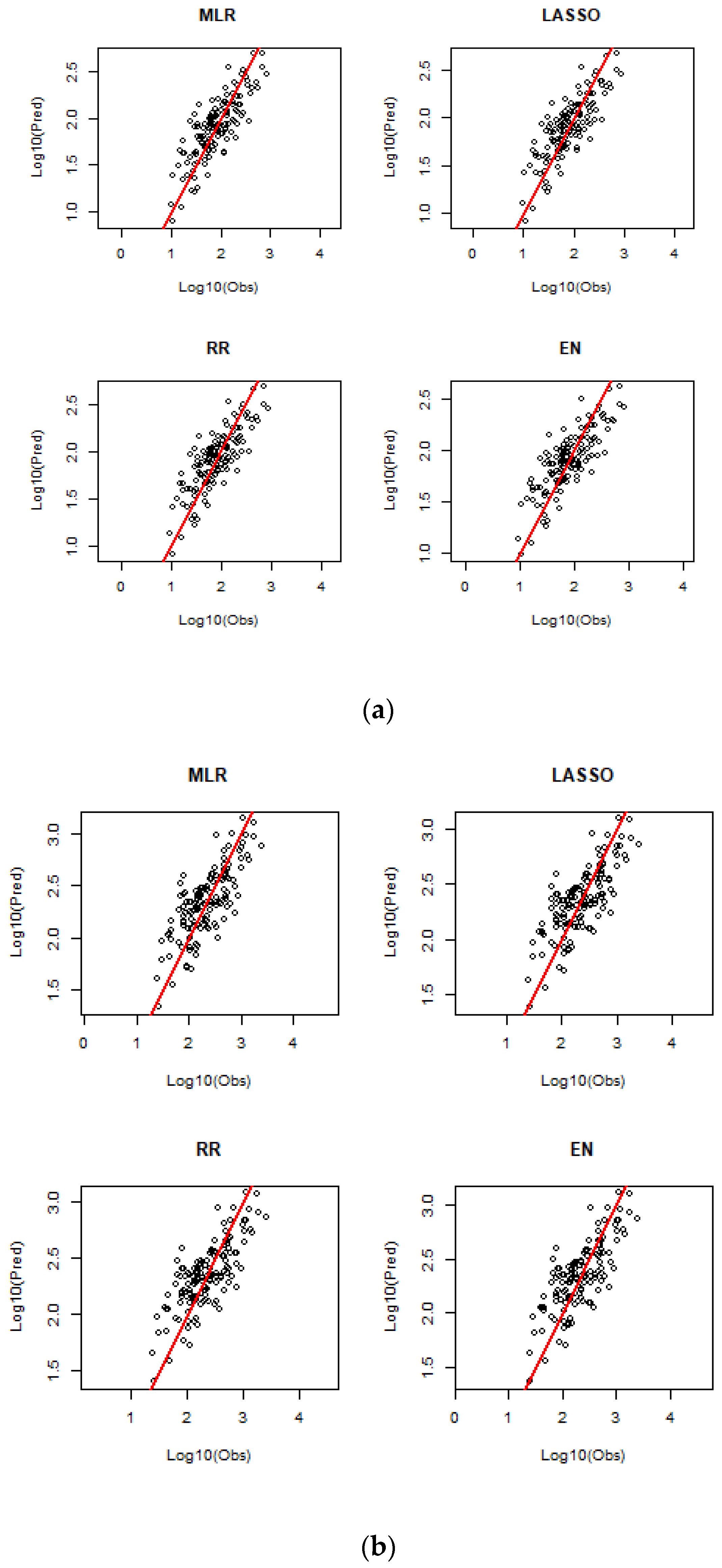
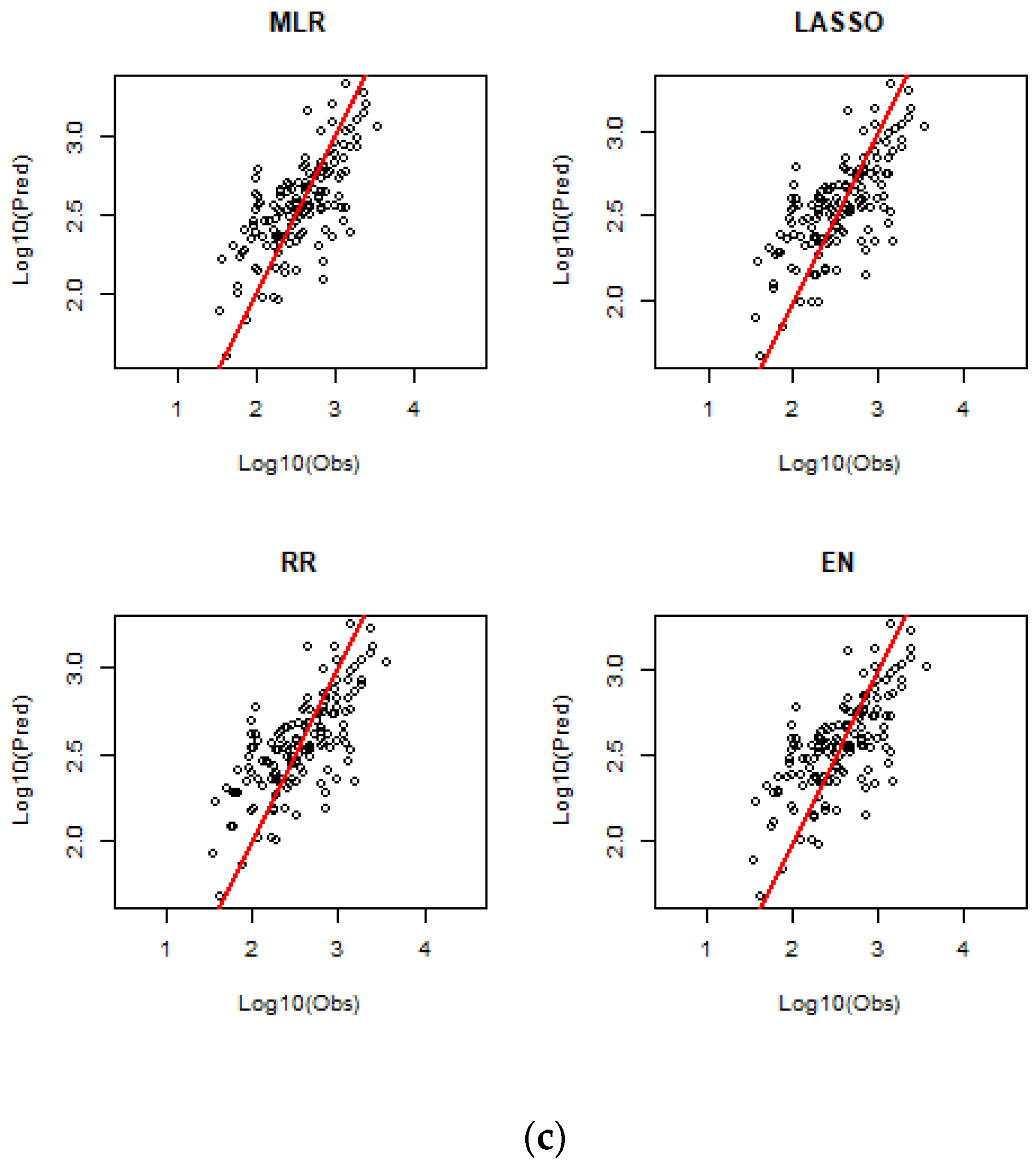
The developed prediction equations contained seven predictor variables; among these, A was the most important predictor, followed by MAR, SDEN, MAE, S1085, FST and SF. The predicted flood quantiles by the selected regression models were obtained by LOOCV and are compared with the observed flood quantiles in a number of ways, as presented below. The predicted and observed flood quantiles for ARIs of 2, 20 and 100 years are plotted in Figure 3 for different regression techniques. Figure S1 (in the Supplementary Section) shows the plots of the predicted versus observed flood quantiles for ARIs of 5, 10 and 50 years. Overall, all four regression models show a similar degree of scatter around the 45-degree reference line. However, as the ARI increases, the scatter around the 45-degree reference line increases, which indicates that higher ARI quantiles are associated with greater uncertainty. This in particular is true when streamflow data length is limited.

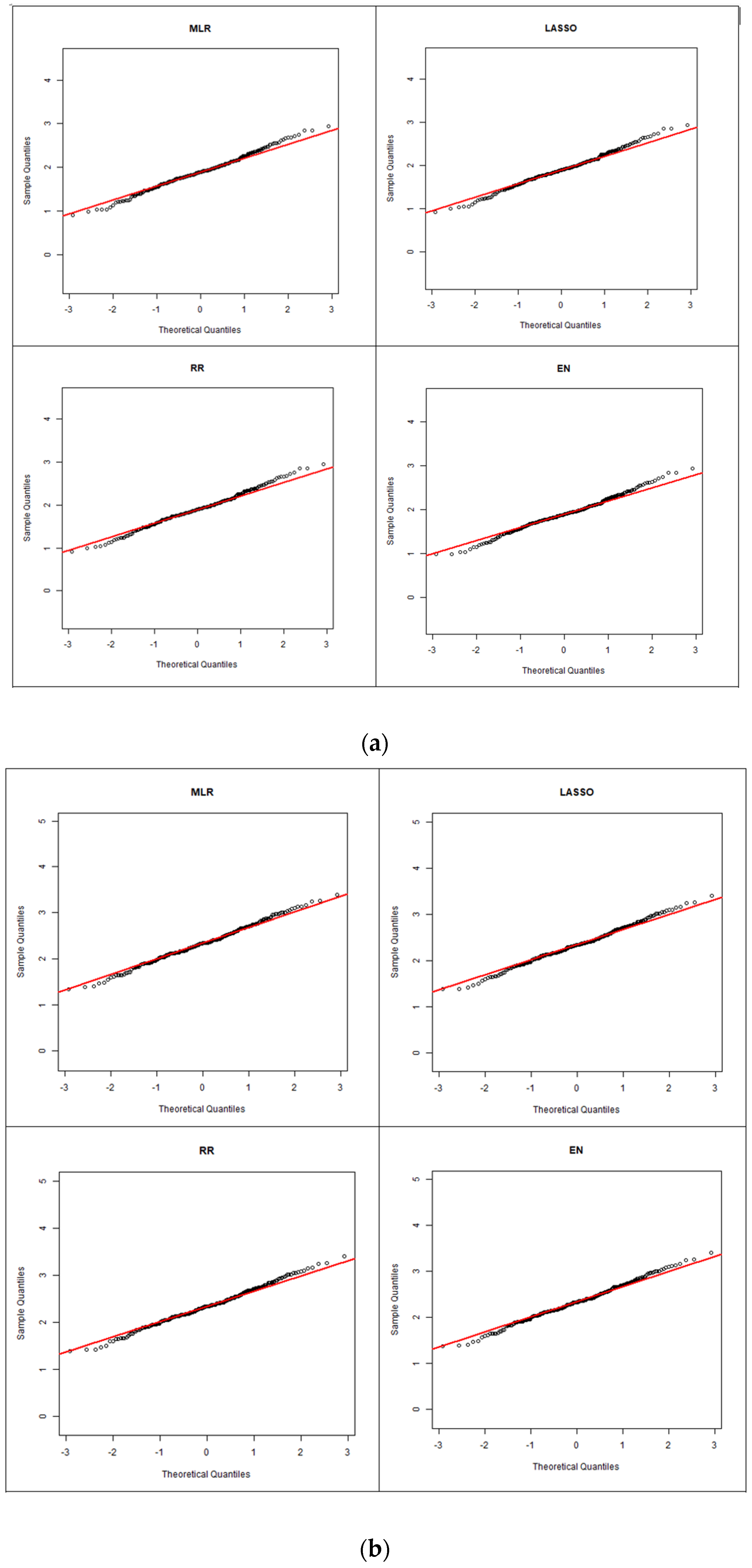
Figure 4 shows the quantile–quantile (Q–Q) plots of the residuals for ARIs of 2, 20 and 100 years for the four regression models (the plots for other ARIs are shown in Figure S2). Upon initial observation, across all the selected ARIs, a relatively linear trend can be found, with most of the data points closely aligned along the 45-degree reference line, which indicates a high degree of agreement between the sample and theoretical distributions of the residuals. This suggests that the underlying model assumption of regression analysis (that residuals are normally distributed) is largely satisfied. It is also found that at a smaller ARI (2 years), there is a large degree of deviation from the reference line, particularly in lower and upper tails of the distribution. Despite the tailed behaviour, across all the selected ARIs, the majority of the data falls into the range of +/−2, which is assuring.

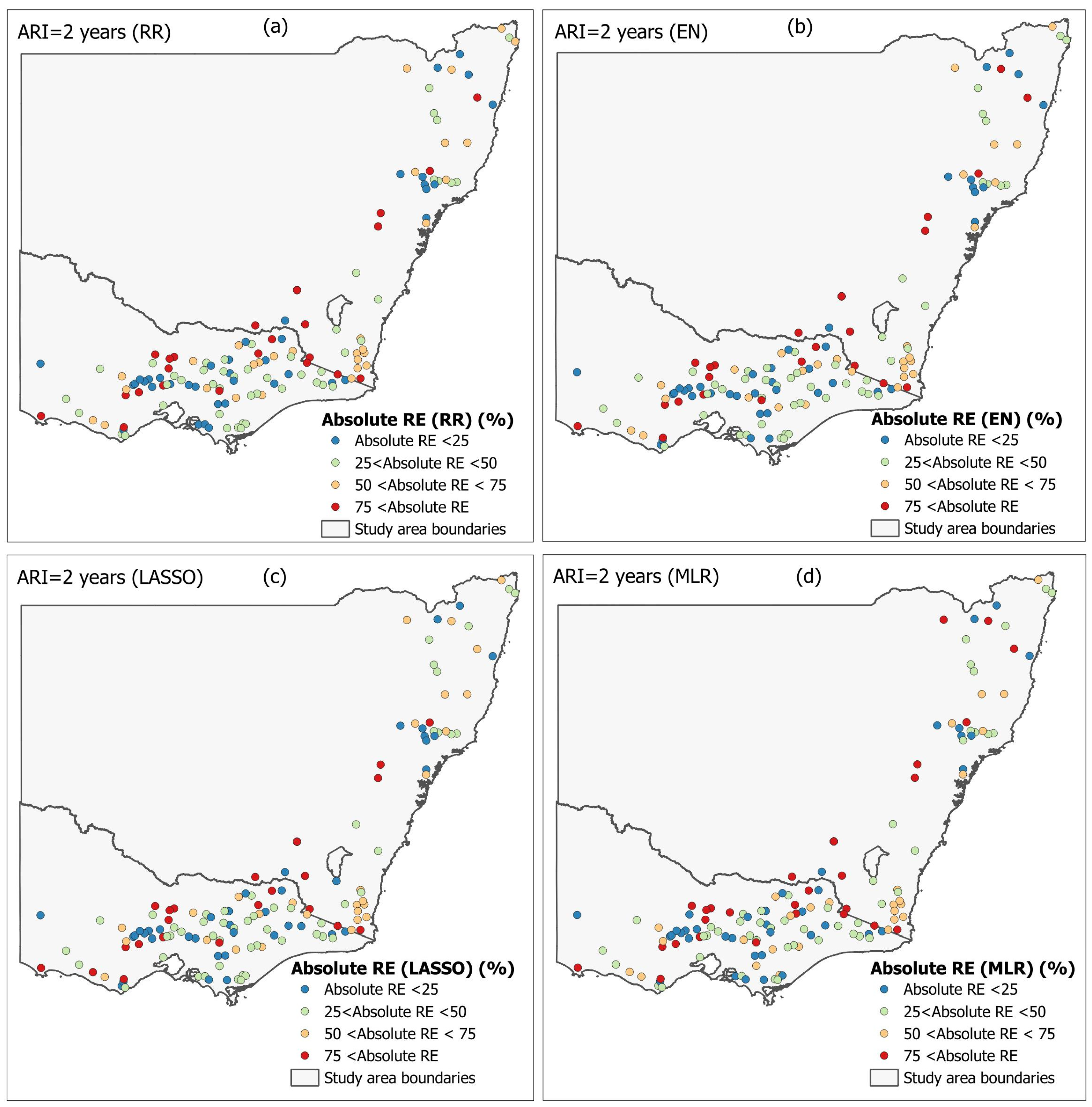
Spatial distribution is widely adopted to visualise the model performance across geographical area. Figure 5 plots the spatial distribution of absolute RE_r values for the 2-year ARI for the four regression models. No significant spatial trend is noticed. There are several stations located in the inland region with very high absolute RE_r for both NSW and VIC. A similar pattern is also observed at the state boundary between NSW and VIC in the coastal region. Further study is needed to identify why these stations are associated with higher RE_r. It should be noted that the RFFA model recommended in ARR showed similar results; i.e., some stations had higher RE_r values in model validation [35]. A slightly higher value for RE_r is observed for the MLR model, which is located in the upper region of NSW.

Figure 6 plots absolute RE_r values for the selected regression models for the 20-year ARI. A similar spatial distribution is observed between MLR and penalised regression models. A few stations located along the coastline of southern VIC are found to have a larger value for RE_r, in particular for MLR and LASSO. Further study is needed to find out the reason for these higher RE_r values. A larger portion of the inland region in VIC is found to have a greater RE_r value for the 20-year ARI. On the other hand, the spatial plot of the 20-year ARI is identical to the 2-year ARI at the boundary between NSW and VIC. Figures S3 and S4 plot the absolute RE_r values for ARIs of 5 and 10 years, respectively. A similar distribution pattern of REr values is observed in coastal regions of the selected stations for these ARIs. In Figures S3 and S4, there are a few stations with larger values of absolute RE_r, unlike Figure 5.

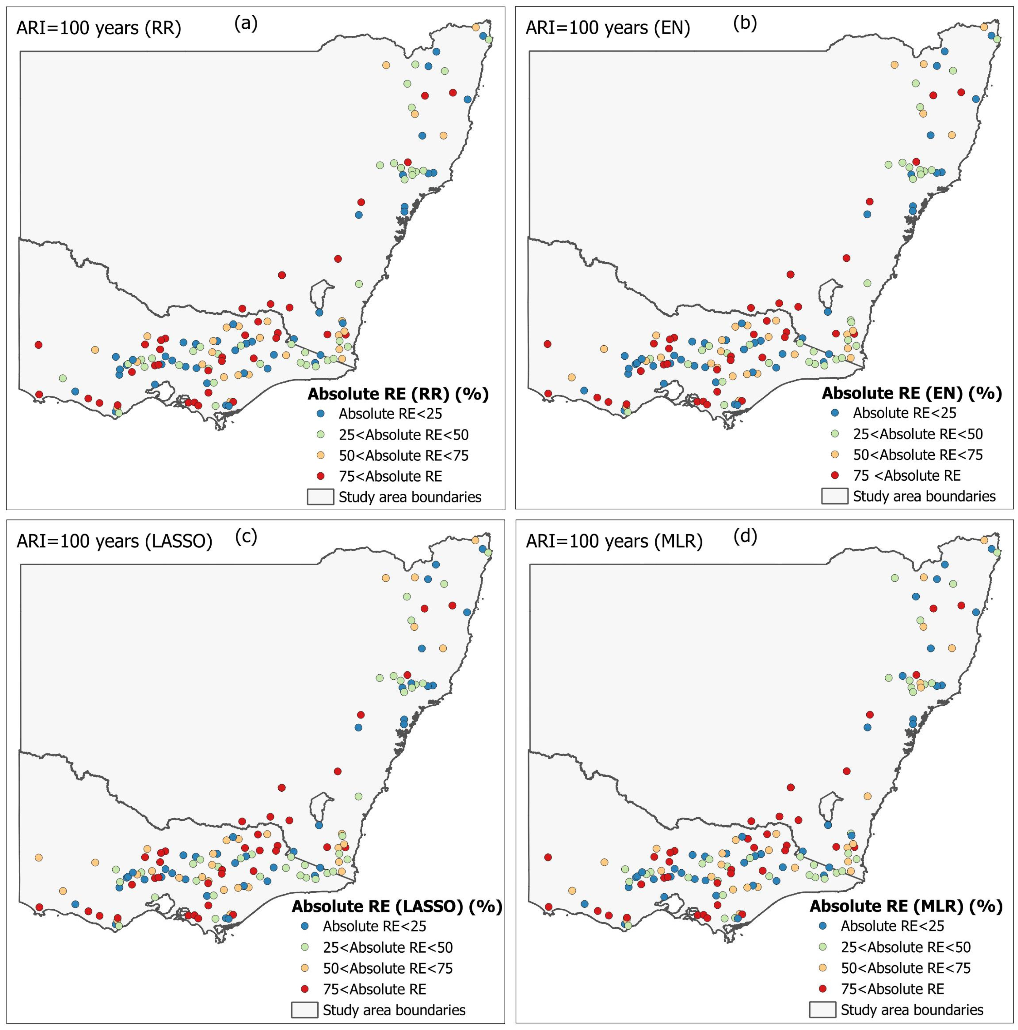
Figure 6 and Figure 7 plot the spatial distribution of absolute RE_r values for the 20- and 100-year ARIs, respectively. A broad agreement between the penalised regression models is found for both of these ARIs. In contrast, the traditional MLR model shows a slight reduction in absolute RE_r for the inland region of VIC. Figure S5 plots the absolute RE_r for the 50-year ARI, which shows a similar pattern as ARIs of 20 and 100 years. Overall, the difference in absolute RE_r across selected regression models is minimal, as can be seen in Figure 8.

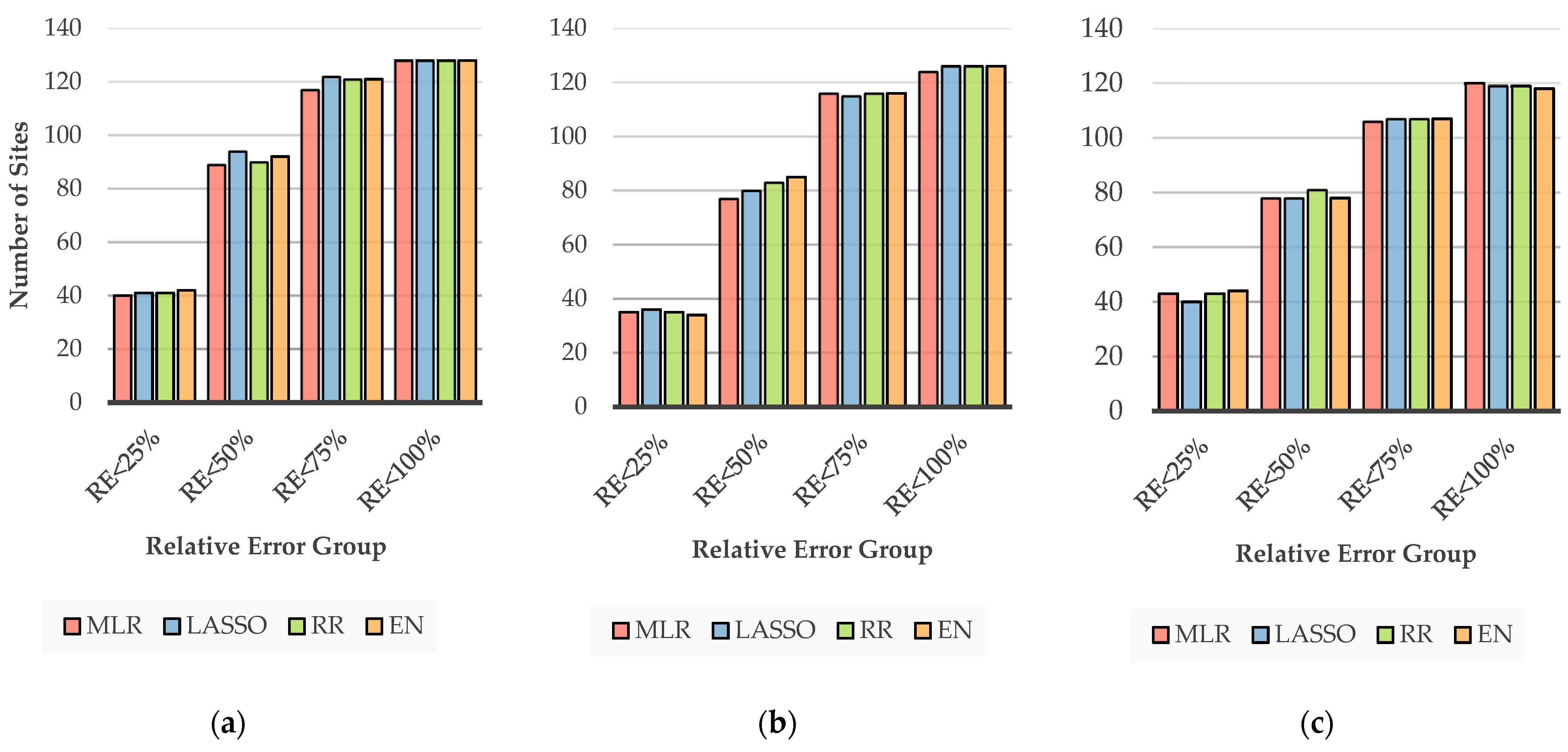
Figure 8 illustrates the cumulative count of sites based on different ranges of absolute RE_r values for ARIs of 2, 20 and 100 years. There are four classes based on a 25% interval of absolute RE_r values. Overall, broad agreement between MLR and penalised regression models can be seen across all the selected ranges of absolute RE_r. For the 2-year ARI, the MLR model accounts for a minimum of 40 stations (RE_r < 25%), while the EN model accounts for 42 stations. A small variability across all the selected ARIs of the stations counted is noted for all four regression models. Figure S6 plots the cumulative site count for ARIs of 5, 10 and 50 years for all the selected regression models. A distribution similar to that in Figure 8 is identified in Figure S6.

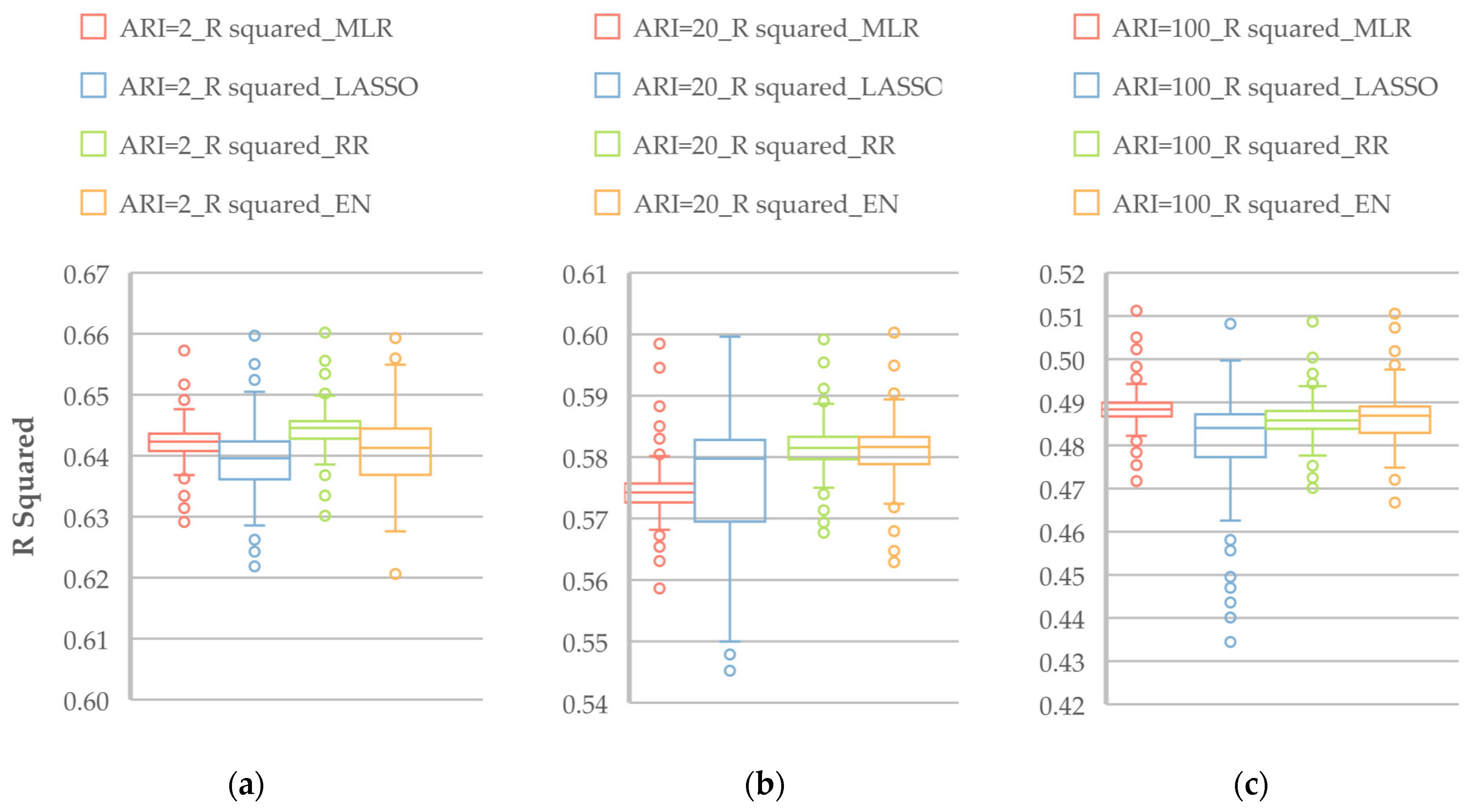
Figure 9 illustrates the R² values of the selected regression models based on LOOCV for ARIs of 2, 20 and 100 years. Among various regression models for the 2-year ARI, MLR shows a median R² of 0.642, while the LASSO and EN models show a slightly reduced value. The RR model shows a median R² value of 0.645. For the 20-year ARI, the MLR model has the lowest median R² value of 0.575, while all the penalised models show median R² values larger than 0.58. Based on the distribution of R² in the boxplots, for the 2-year ARI, the best model is RR, which is followed by MLR, EN and LASSO. For the 20-year ARI, the best model is RR, which is followed by EN, LASSO and MLR. For the 100-year ARI, the best model is MLR, which is followed by RR, EN and LASSO. Figure S7 plots the R² values for the 5-, 10- and 50-year ARIs. Similar to Figure 9, in Figure S7, there is no model showing the best performance across all the ARIs.

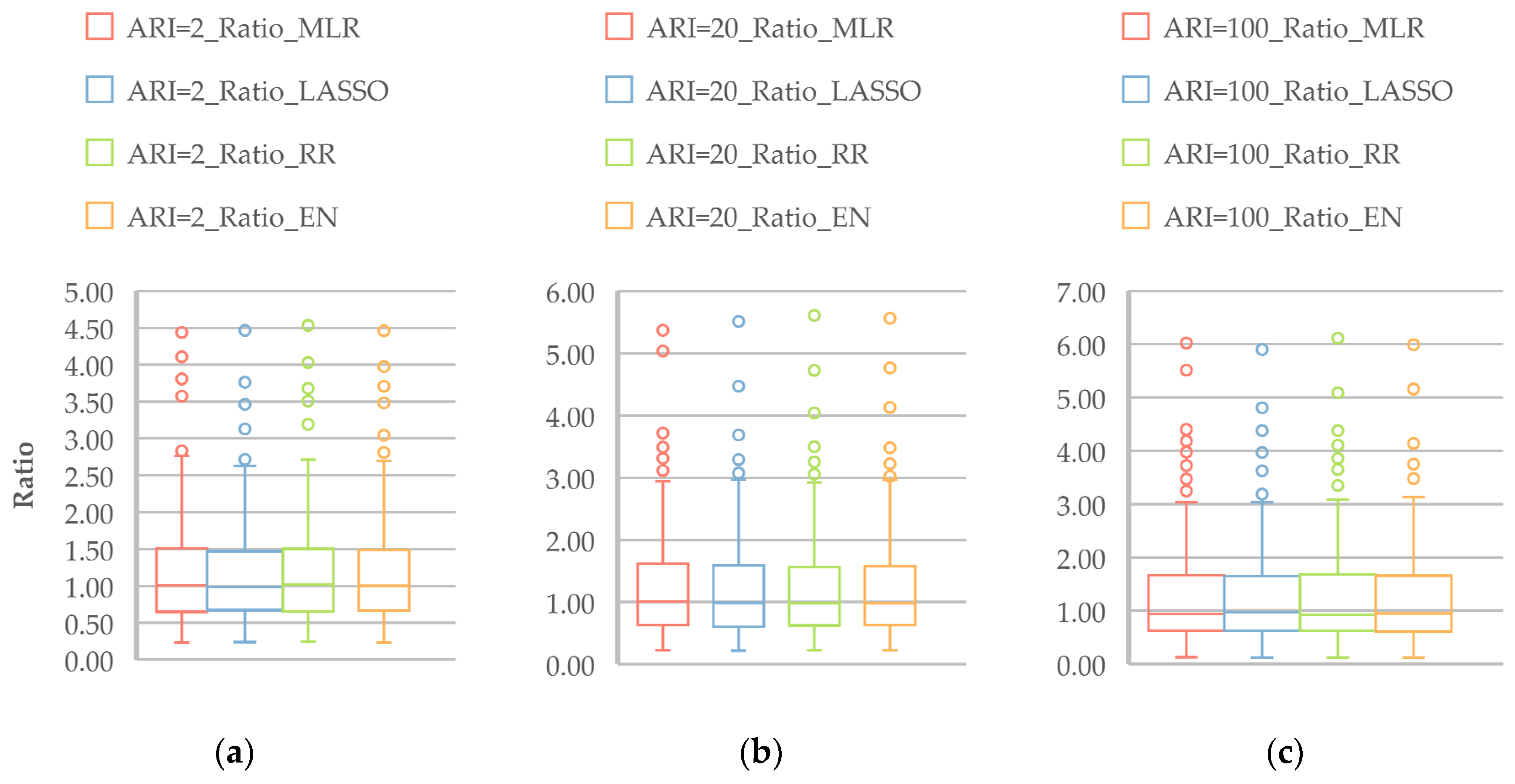
Figure 10 plots the Q_Pred/Q_Obs ratio (Equation (7)) for the regression models for ARIs of 2, 20 and 100 years. All the models show a median ratio value around the 1:1 line, which represents a broader agreement between the predicted and observed flood quantiles, without notable bias. Furthermore, the distribution of the ratio values (as shown by the boxplots) for all four models are very similar. Figure S8 plots the ratio values for ARIs of 5, 10 and 50 years, which broadly represent similar results to those in Figure 10.

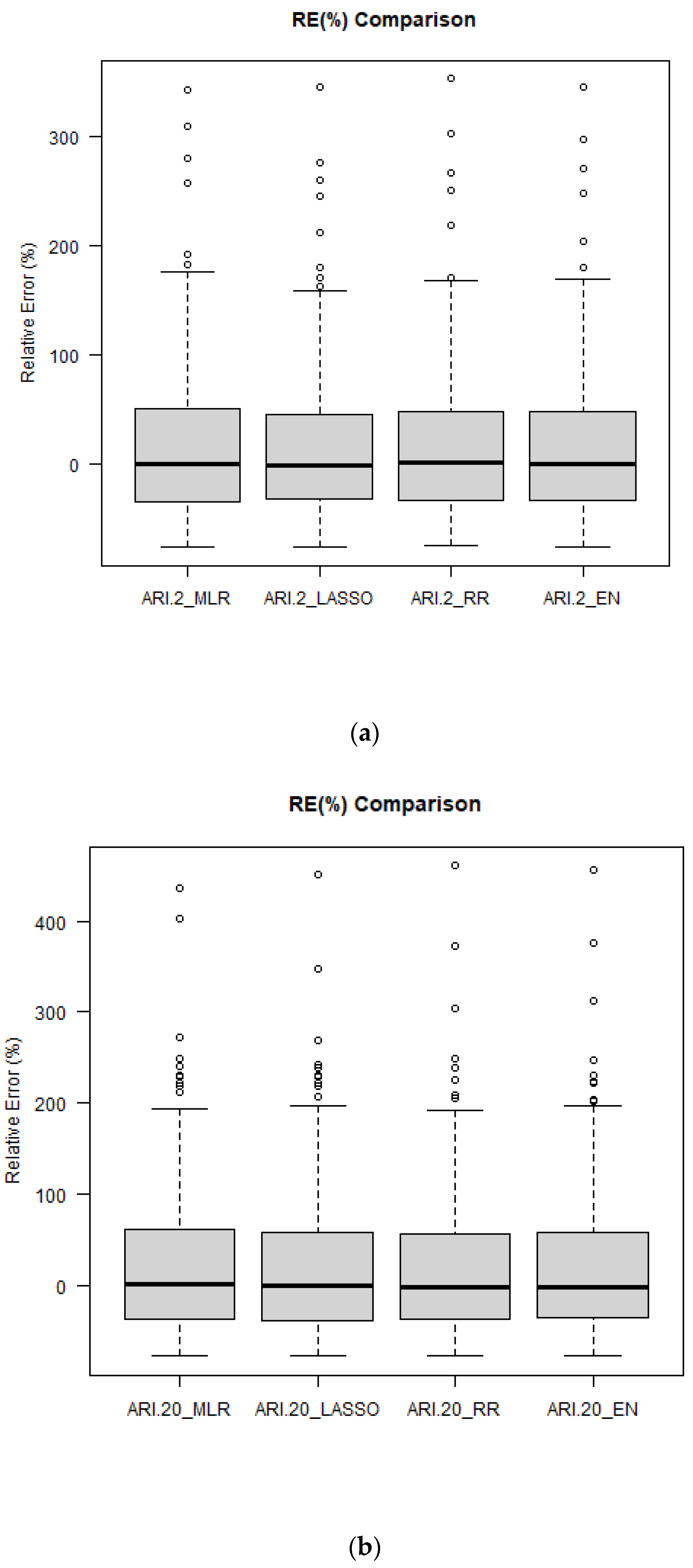
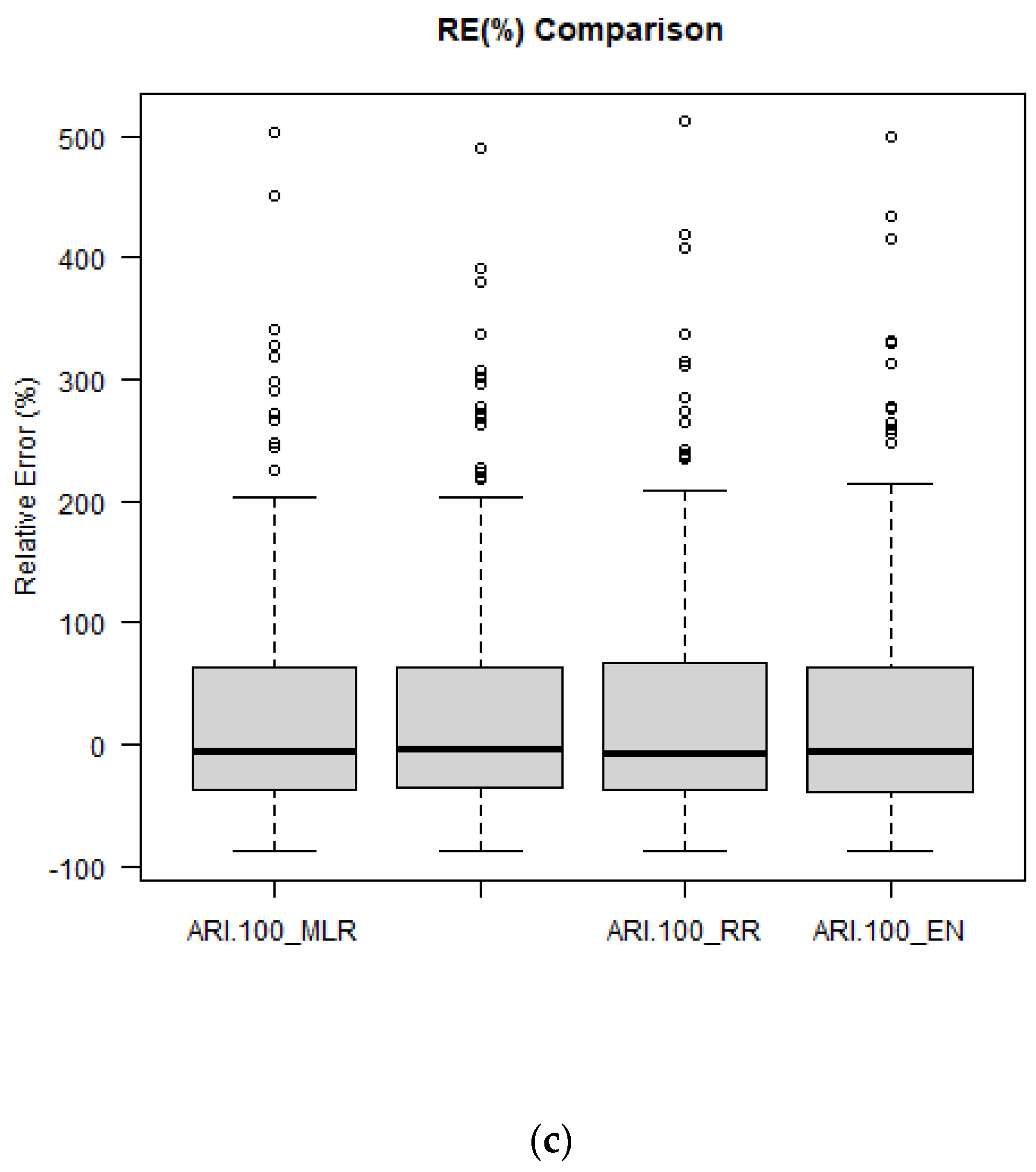
Figure 11 shows the boxplots of RE_r values for ARIs of 2, 20 and 100 years. The median RE_r values match very well with the 0:0 line, which indicates that the developed regression models are mostly unbiased. The distribution of RE_r values is quite similar for all the regression models (a very similar result is noticed for ARIs of 5, 10 and 50 years, as shown in Figure S9). It should be noted that for a few stations all the regression models show an overestimation of the predicted quantiles (shown as outliers in the boxplots).

The RE_m values (Equation (4)) for the four regression models for all six ARIs are shown in

Table 4. Median relative error (RE_m%) values for the four regression models.

ARI (Years)	MLR	LASSO	RR	EN
2	39	37	38	37
5	43	43	43	45
10	44	43	44	46
20	47	44	44	44
50	45	43	43	44
100	44	46	46	47

. Although the RE_m values are not remarkably different across the four regression models, LASSO has the smallest RE_m values overall. The RE_m values for LASSO are 37%, 44%, 43%, 44%, 43% and 46%, which are generally smaller than similar RFFA studies, such as that by Zalnezhad et al. [21], who reported RE_m values of 42%, 33%, 36%, 40%, 44% and 54% for ARIs of 2, 5, 10, 20, 50 and 100 years, respectively, for an artificial neural networks (ANN)-AM-based RFFA model for south-east Australia. Zalnezhad et al. [21] reported median Q_Pred/Q_Obs ratio values in the range of 0.94 to 1.57, which are very close to 1.00 in this study. The RE_m values for LASSO are also smaller than those recommended by the Australian Rainfall and Runoff AM-based RFFA model [35], which reported RE_m values in the range of 57–64% for ARIs of 2 to 100 years. The current study provides a more accurate prediction than the study of Aziz et al. [36], who reported RE_m values in the range of 39% to 91% and median Q_Pred/Q_Obs ratio values in the range of 0.17 and 1.82 for an ANN-AM-based RFFA model in south-east Australia.

4. Conclusions

The study presents the development of POT-based RFFA models for south-east Australia, using regularised linear models (least absolute shrinkage and selection operator (LASSO), ridge regression (RR) and elastic net regression (EN)). It has been found that the regularised linear models provide more accurate flood quantile estimates (with a median relative error in the range of 37 to 47%) as compared to the AM-based RFFA techniques currently recommended in the Australian Rainfall and Runoff guideline. The results of our study provide valuable insights into the performance of regularised linear models in the context of RFFA and highlight the potential benefits of incorporating these models within the POT framework. Our findings contribute to the ongoing efforts to improve the accuracy and reliability of POT-based RFFA, which is crucial for effective flood risk management and decision-making, in particular for smaller return periods. These regularised linear models should be tested in other Australian states, using both the AM and POT models, and should be compared with existing RFFA techniques, which will assist in recommending a more accurate RFFA technique for Australia.