Abstract
This paper uses the SPH method to study snow disasters, including the snow flow model of a vertical water diffusion equation and heat balance equation. The advantage of the SPH method is that it can capture particles’ positions, which can be used to track the initial position distribution of hazardous particles. At the same time, a particle modeling method based on pixel value is proposed, which has certain advantages in dealing with the boundary modeling of different materials. In addition, snow disaster prevention and the control of classic embankment and cutting procedures were carried out. The final treatment results showed that the number of snow particles on the subgrade surface was reduced by about 90%. The validity and feasibility of the snow disaster simulation software based on the SPH method are verified by comparison with the experimental results.
1. Introduction
Snow cover is an important part of the cryosphere and has unique thermodynamic and hydrological characteristics. Its sublimation process is an important factor affecting the global water vapor balance and atmospheric circulation and significantly impacts global ecology, hydrology, atmosphere, and geomorphology [1,2]. The most active element in the cryosphere is snow, and each year it covers up to one quarter of the surface of the Earth. Snow cover has the characteristics of uneven spatial distribution and rapid spatial and temporal changes, especially in mountainous areas with complex terrain [3,4]. Snow is more likely to occur than ice sheets and it is more widely distributed.
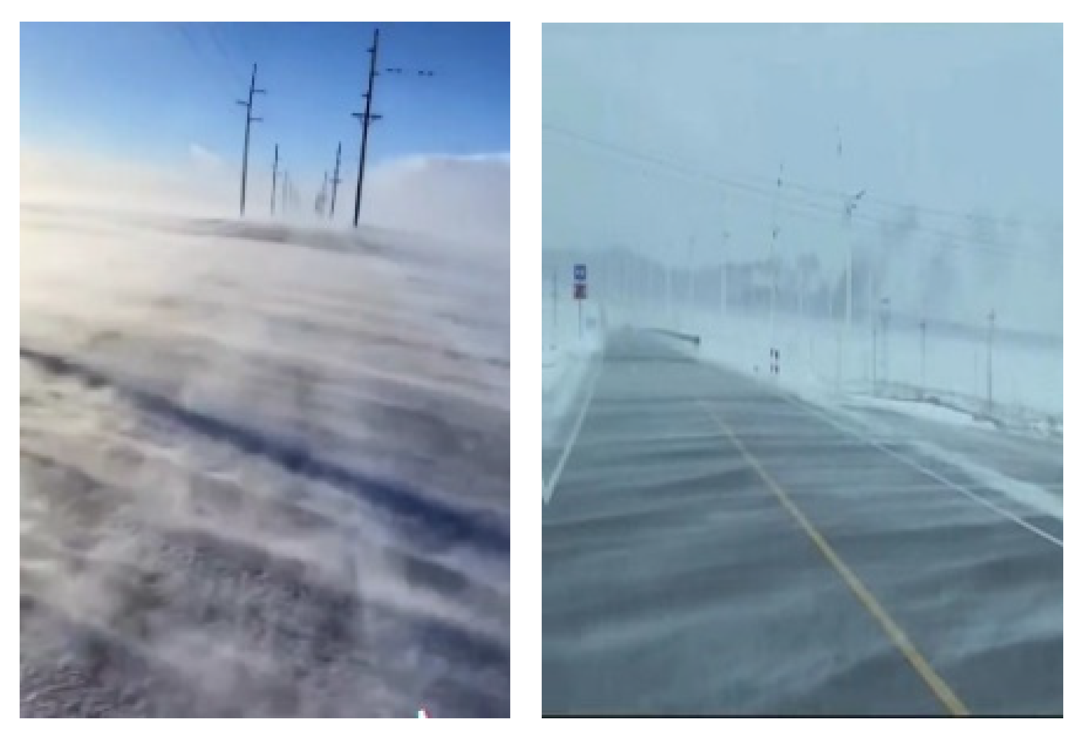
Blowing snow is widely distributed in China. The trend of snow distribution in China is to thicken from south to north, and the snow distribution grows thicker as altitude increases. In Xinjiang’s southeastern and southwestern regions, the snow cover is the thickest, reaching a maximum of more than 1.2 m. Snow disasters seriously affect the development of China’s economy. As shown in Figure 1, wind-blown snow has a very important impact on human life; therefore, it is very important to study the process of snow flow formation to prevent snow disasters.
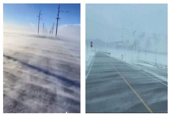
Figure 1.
The hazards of wind-blown snow.
The study of snowdrifts is mainly conducted vis wind tunnel tests, field observations, and numerical simulations. With the rapid development of computers, the results of numerical simulations are becoming more and more accurate. Some scholars have observed that differences in the shapes of snow particles can significantly influence the amount of stagnant snow due to various air drag forces [5]. Historically, most value simulation studies regarded snow particles as spherical. However, as more in-depth research on snow–wind flow has emerged, people have come to realize that the influence of wind and snow sublimation cannot be ignored. In 2009, Wever et al. first recorded the sublimation rate of snow particles in a closed wind tunnel test [6]. With the development of computer technology and the theory of snow flow, most scholars now use numerical simulation to simulate the complex physical process of snow sublimation [7,8,9]. According to previous research conclusions, an adequate water transport mechanism can significantly weaken the negative feedback effect of sublimation. Due to the large density of snow particles in the saltation layer, the volume sublimation rate is much higher than that of the suspended layer [10].
The two main current snowdrift models are the two-fluid model and the Euler–Lagrange model [11]. The two-fluid model ignores the motion state of snow particles; thus, it is unable to simulate the physical properties of snow particles during motion. Conversely, although the Euler–Lagrangian model can describe the movement of snow particles, it requires high grid accuracy for small-sized snow particles and is difficult to implement in actual calculations. A comprehensive model combining saltation and the suspension motion of snow particles avoids the shortcomings of the first two models; however, it still overlooks the process of salting snow, which involves collisions and splashing, as well as the change in mass that results from snow sublimation. The formation of snow–wind flow involves a complex process of multi-field couplings such as wind field–snow particle–temperature and humidity. At present, a systematic solution has yet to be introduced.
The manifestation of snow disasters on traffic routes can be divided into two aspects: 1—Traffic congestion caused by snow. 2—Wind-blown snow increasing the concentration of snow particles in the air, resulting in reduced visibility. In past studies on roads, various snow barrier conditions were established first. Then, numerical simulations or wind tunnel experiments were carried out to reach conclusions regarding the optimal snow protection effect for a specific condition. However, traditional research methods consume a lot of time and may not be pertinent.
In this paper, the smoothed particle hydrodynamics (SPH) method is used to numerically simulate the movement of snow particles in the wind–snow two-phase flow, which avoids various problems such as distortion caused by the large deformation of the grid method, and which has unique advantages in tracking the trajectory of particles and the change in physical properties [12,13,14,15]. The SPH method’s fundamental tenet is to divide the computing domain into separate particles. The distinct features of snow particles in nature are consistent with this property. These snow particles carrying their physical characteristics can move with the control equation. Different smooth lengths are used for different phases in the wind–snow two-phase flow, which can solve the problem of coupling between snow particles and between snow and air particles. According to the influence particles in the influence domain, the momentum of the target particles is recalculated so that the collision and splashing processes of snow can be regarded. At the same time, the physical information of snow particles and the air is recalculated, such as the speed, position, and mass of snow particles and the speed, position, temperature, and humidity of air particles.
2. Introduction of SPH Equations
2.1. Basic SPH Method Equations
The SPH approach typically consists of two basic steps: particle representation and integral representation, sometimes referred to as the approach of approximating the field function kernel [10]. The integral representation of the function in the SPH technique is as follows:
where is the integral volume containing , and is the Dirac function. It has the following properties: (1) ,; (2) , .
The integral form of the function may be expressed as follows by swapping out the Dirac function with the smooth function :
The approximation at particle can be expressed as follows:
where is the kernel function and is the smooth length. The superposition of the values of the adjacent particles is approximated, and the function particle approximation can be expressed as follows:
In the formula, , is the distance between particles, , and is the distance between particles and .
The three components of the snowstorm numerical simulation program based on the SPH approach are shown in Figure 2. In addition to creating virtual particle–solid wall borders, pre-treatment may also create air and snow particles. Air particles are given physical attributes like velocity, temperature, humidity, and density, whereas snow particles are given physical properties like density, velocity, and viscosity. By calculating the particles carrying the material attributes, the main processing updates the information on the particles’ temperature, humidity, speed, and location. The major purpose of post-processing is to make it possible to see the results of calculations.
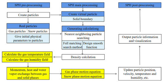
Figure 2.
SPH method snow flow numerical simulation flow chart.
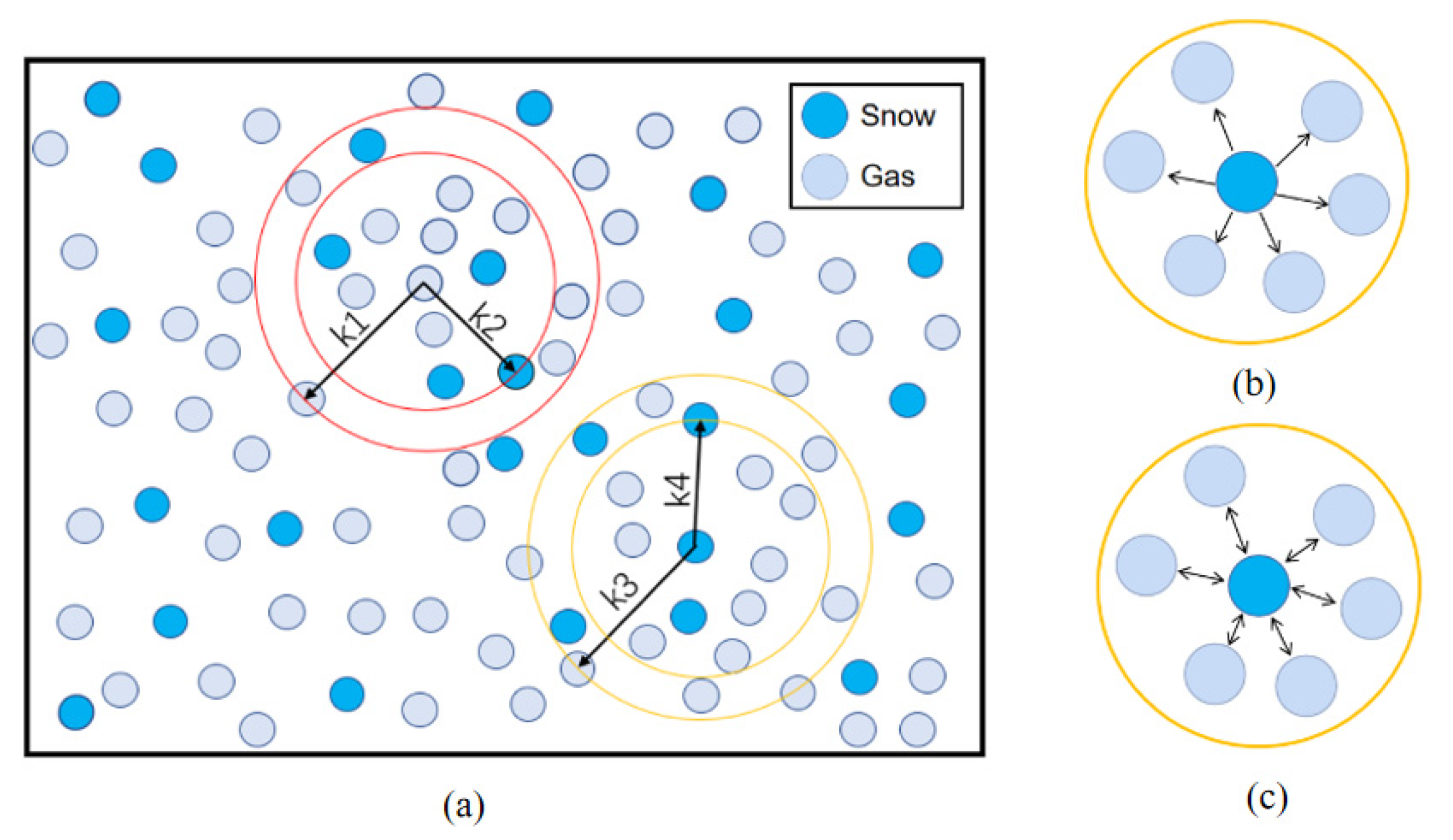
2.2. Smooth Radius and Support Domain
In the example, the support domain of the particles is set to be circular, as shown in Figure 3a. The target particle, which is the particle in the center of the circle, will be impacted by the particles in the support domain with a radius. The smoothing factor, where h is equal to the particle diameter, is the product of the smoothing length and the support domain radius. The interaction between snow and air particles must be addressed since they have a mutually beneficial influence.
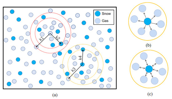
Figure 3.
Support domain of particles. (a) Support domain. (b) Water vapor diffusion. (c) Heat transfer.
The snow sublimation process is shown in Figure 3b. Snow particles sublimate from solid to gas, and the generated water vapor will give air particles in the support domain and increase the air’s water vapor content. As demonstrated in Figure 3c, the air temperature drops due to heat being transmitted with the air particles in the support domain during the sublimation of snow.
2.3. Kernel Function
The quintic spline function is as follows:
The gas treatment is incompressible Newtonian fluid treatment. The motion of snow is a near-surface motion, so its motion control equation mainly considers mass conservation and momentum conservation [8].
3. The Control Formula of Snow
Aerodynamic drag is
where .
The velocity after collision [15] is
3.1. Model Initial Conditions
The boundary conditions are
Initial gas velocity is
where the friction wind speed is and the aerodynamic roughness is .
The initial absolute temperature is
where the initial temperature is and the atmospheric pressure is .
The initial atmospheric pressure is
where .
Initial humidity is
where .
3.2. Snow Particle Sublimation Control Formula
The following is the snow sublimation equation [16]:
where is the Nusselt number and is the Sherwood number.
The temperature and relative humidity equations [17] are the following:
where is the rate at which snow volume sublimates and is the water vapour diffusion coefficient.
where .
3.3. Computational Parameters
Other calculation parameters used in the calculation of this model are shown in Table 1.

Table 1.
Other calculation parameters.
4. The Control Formula of Snow
In calculating SPH, the vital step is to discretize the problem domain with particles; establishing the initial model has a specific influence on the accuracy of the calculation results. The establishment of the traditional SPH initial model is generally based on the design of particular algorithms and procedures for specific problems, and this method undoubtedly increases the difficulty of particle generation for complex models. Therefore, it is of great significance for the research of SPH to innovate the pre-treatment part and thereby improve the generation efficiency of pre-treatment model particles.
4.1. Pixel Value Conversion
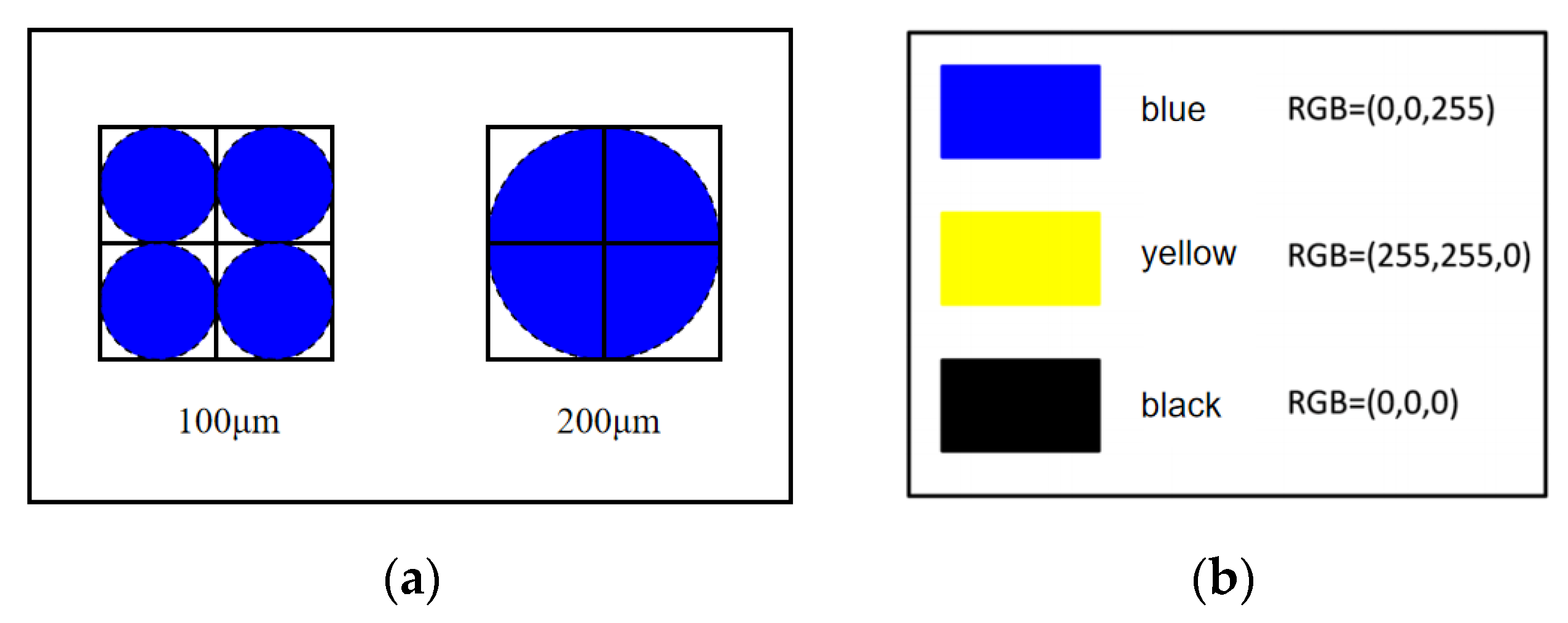
Drawing software or modeling software is used to establish the desired model size and shape for the generation of a two-dimensional SPH model. Then, the drawn model is exported as a photo form such as jpg or png. The matter of the model picture is filled with different colors, and the size of the image pixels is proportional to the desired model size so that the conversion of particles is convenient.
The processed picture is imported into the pre-processing program to generate the SPH particle position, wind speed, temperature, humidity, and other information. Pre-processing is mainly used to identify the RGB value of the pixel, and the color setting has no significant influence, as shown in Figure 4b. The two-phase flow of wind and snow mainly involves the establishment of the gas phase, solid phase, and virtual particles, in which blue represents air, yellow represents snow particles, and black represents virtual particles.
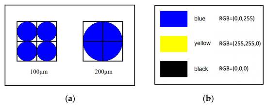
Figure 4.
Conversion of pixel value and particle. (a) Pixels convert particles. (b) Pigment value.
To facilitate the calculation, a pixel is generally established as a particle with a diameter of 100 μm. If the particle diameter is 200 μm, four pixels specify a particle, as shown in Figure 4a. If you want to improve modeling accuracy, you can use larger pixel values. On the contrary, the model can be scaled down to a smaller pixel-value photo to enhance computational efficiency.
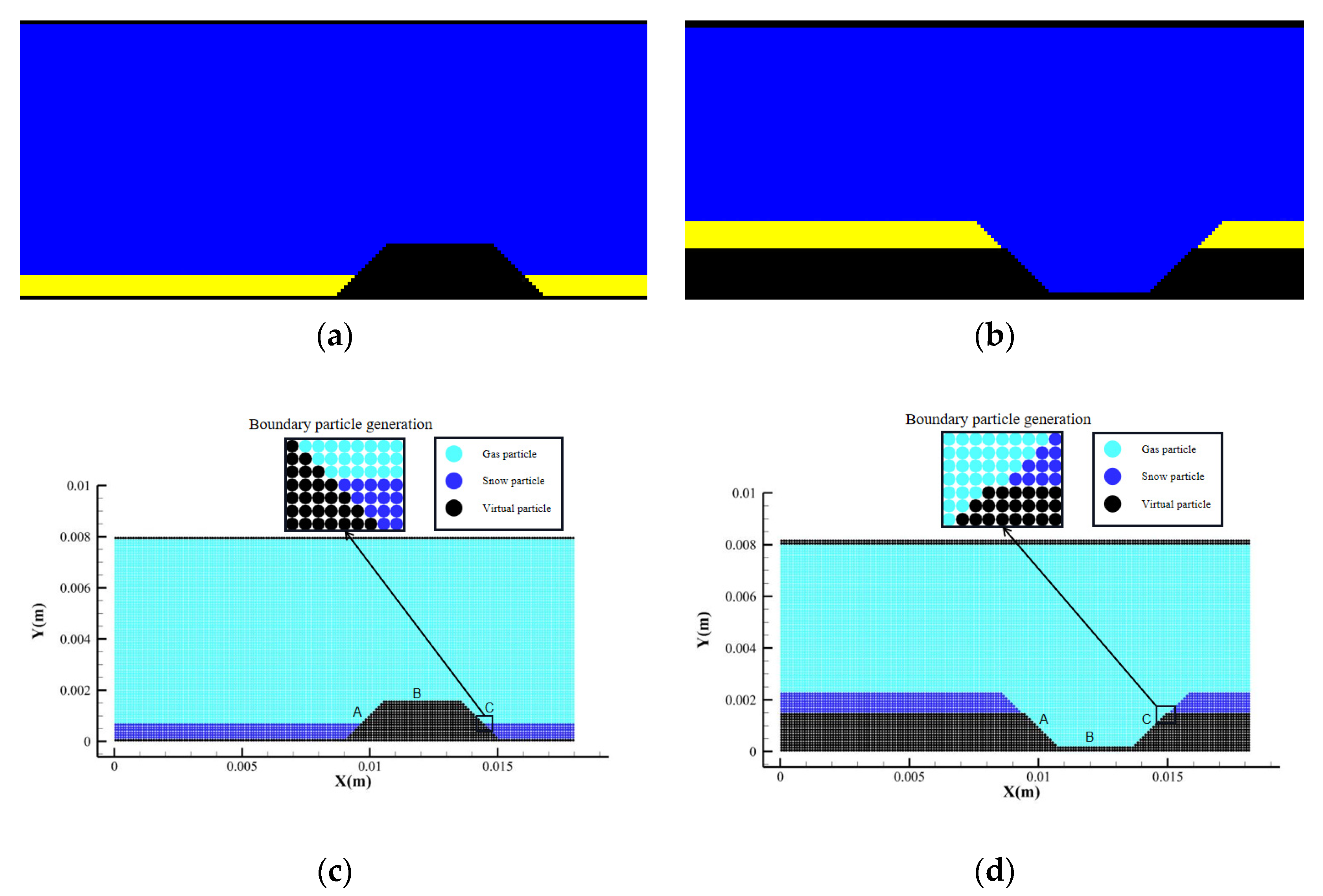
4.2. Particle Generation of Embankment and Cutting Models
Figure 5a,b are embankment models drawn by drawing software and saved in png format. Figure 5c,d are the initial models transformed into SPH particles via pre-processing. The particles at the boundary of three different substances are arranged neatly, and the precision of particle generation is high. Compared with the traditional SPH modeling method, the model generation speed and accuracy are faster.
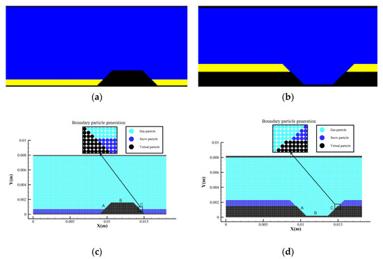
Figure 5.
Establishment of initial model. (a) Embankment picture. (b) Cutting picture. (c) Embankment particle conversion. (d) Cutting particle conversion.
4.3. Particle Generation of Complex Particle Size Models of Flat Snow Beds
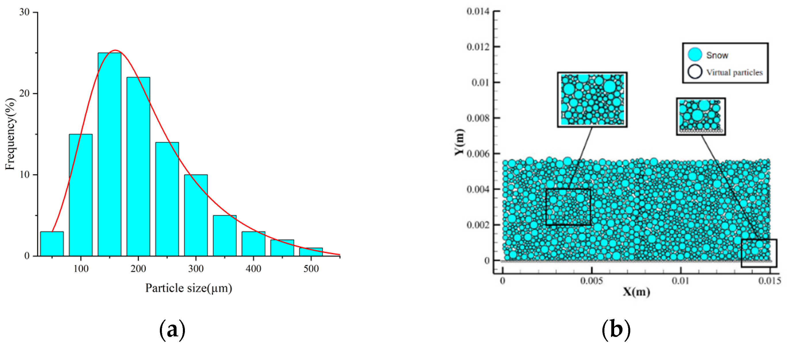
Figure 6 shows that the probability distribution of the adequate particle size of the wind-blown snow movement satisfies the gamma distribution and the normal distribution [12,18]. The region of the snow bed is judged by the pixel value, and the snow particles are generated according to the actual particle size ratio, which is more in line with the distribution law of a natural snow bed. After the particle generation is completed, the overlap and gap judgments are made. After that, to meet the natural stress situation of the snow particles on the snow bed, gravity and collision force are applied to the snow particles for re-stacking, as shown in Figure 6b.
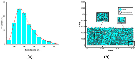
Figure 6.
Establishment of multi-particle size model. (a) Effective particle size distribution of wind-blowing snow. (b) Multi-particle size model.
5. Model Verification and Result Analysis
5.1. Model Verification
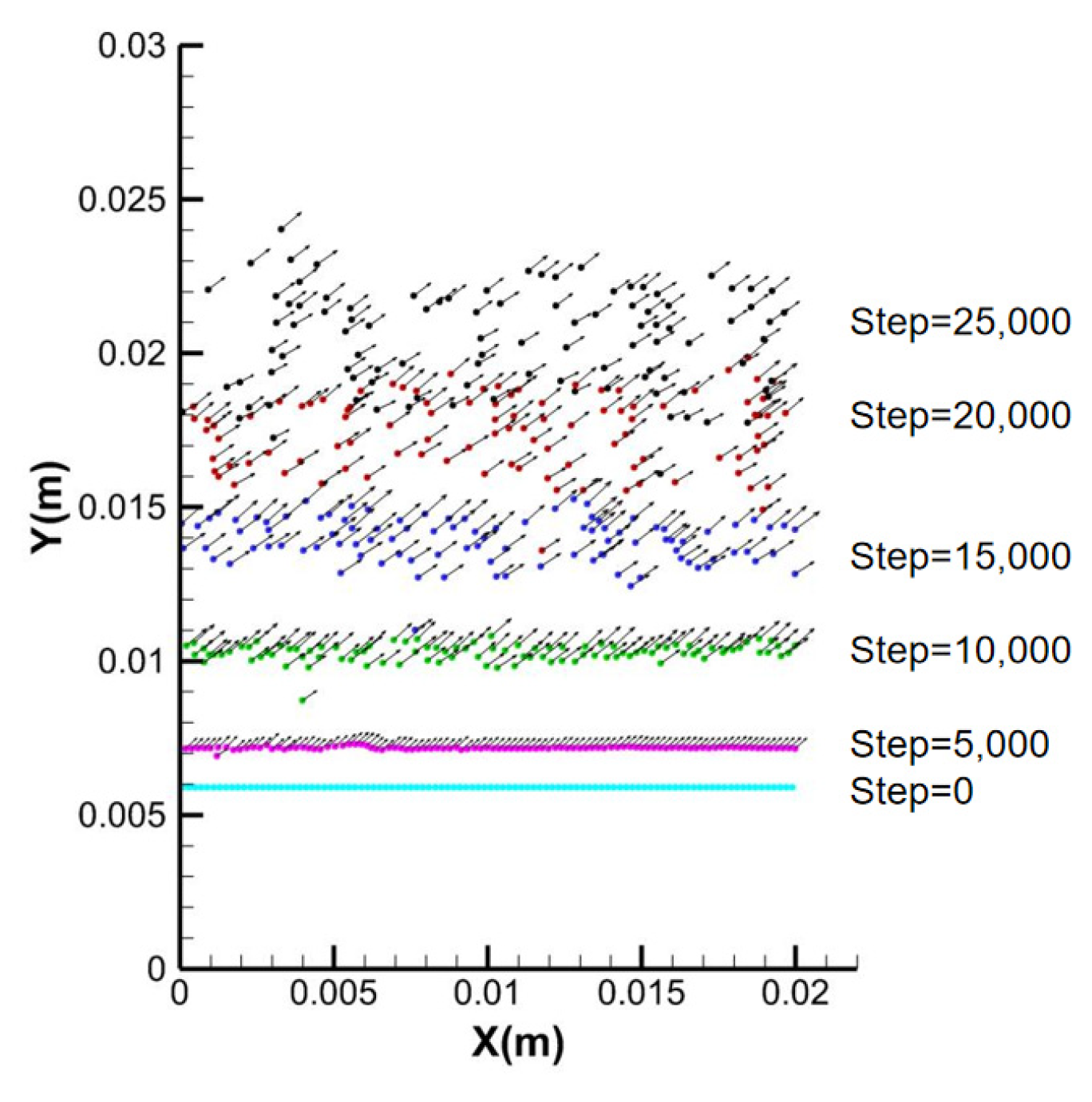
Figure 7 shows the velocity and position changes of the uppermost snow particles. When Step = 0, the snow particles are in a stationary state. Due to the influence of the air drag force, the velocity of the snow particles is greater than the critical speed of its start, resulting in a pace with little difference in size and direction, as shown in Step = 5000. When Step = 10,000, the size and direction of snow particle velocity in the same layer begin to differ. When air particles act on snow particles, they are also subjected to the reaction force of snow particles. The reaction force causes changes in the flow field near the snow particles because the airflow disorder will exert different external forces on the nearby snow particles. This leads to the difference in the size and direction of snow particle velocity in the same layer. As such repetition occurs, the speed and position of the same layer of snow particles gradually begin to change differently, such as Step = 15,000, Step = 20,000, Step = 25,000. At the same time, the speed and position change, and the flow field, temperature, and humidity around the snow particles will also change differently. This leads to the difference in snow sublimation rate.
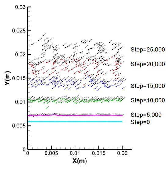
Figure 7.
Changes in velocity and position of the uppermost snow particles during take-off.
The probability distribution of the speed of traveling snow particles at three distinct frictional wind speeds is determined, as shown in Figure 8. The distribution probability of the resultant velocity obtained by fitting in this study satisfies the Gauss distribution (22). The distribution characteristics obtained from the wind tunnel test data of Lv (2012) are in good agreement, which verifies the accuracy of the SPH snowstorm flow model [19].
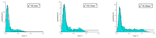
Figure 8.
Probability distribution of upward-moving snow particle velocity.
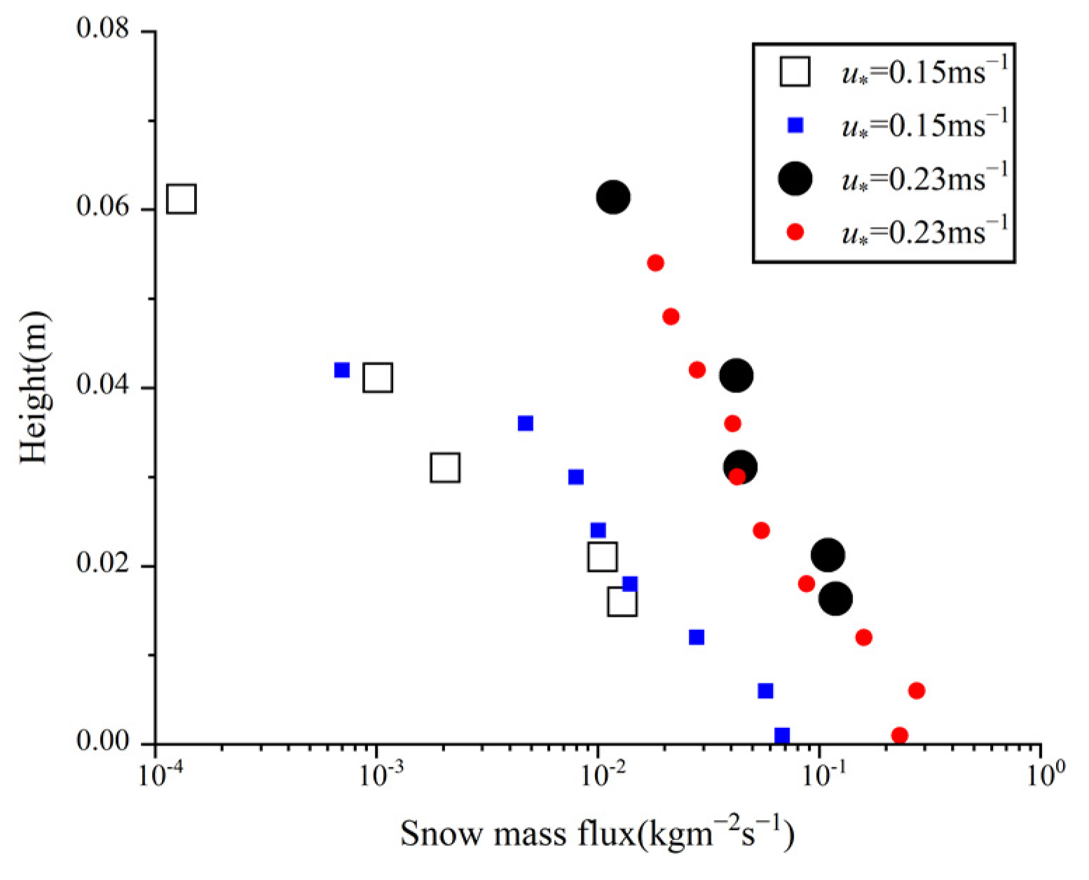
Figure 9 shows the mass flux of the flat snow bed. Both the field measurements of Sugiura (1998) and the modeling findings presented in this work demonstrate exponential attenuation with height [20].
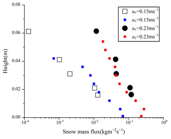
Figure 9.
The flux of snow on a flat surface. Black is an experiment, and the color is a simulation [21].
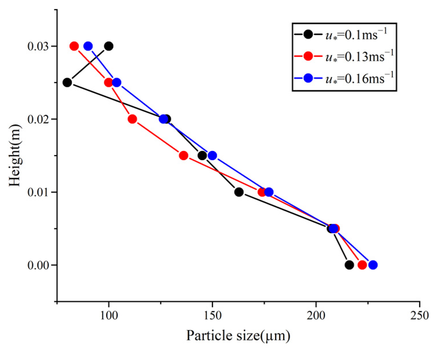
Figure 10 shows the flat snow bed’s average particle size height distribution. The average snow particle size distribution simulated in this paper decreases linearly with the increase in height, which is consistent with the trend of field measurement by Dover (1993) and Gordon (2009) [22,23]. Furthermore, we verified the accuracy and feasibility of the SPH snow flow model.

Figure 10.
Average particle size height distribution of flat snow bed.
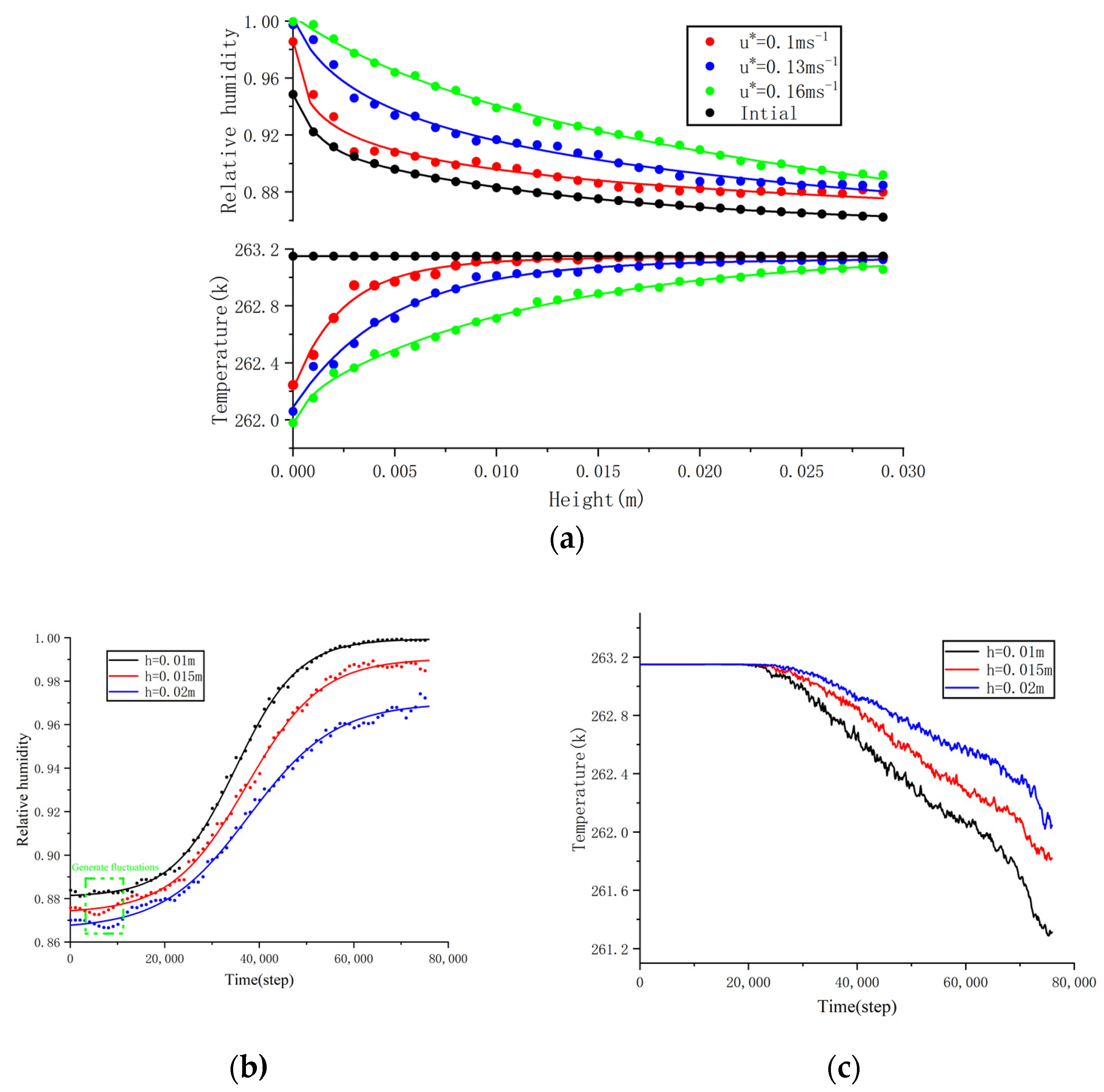
The distribution of temperature and humidity are shown in Figure 11. With increasing friction wind speed, humidity rises, and it decreases with increasing height. The temperature rises with an increase in height while falling with an increase in friction wind speed. The reasons for these phenomena are as follows: (1) Snow sublimation will absorb the heat of the air and release water vapor. (2) With the increase in friction wind speed, the kinetic energy of snow particles increases, which increases the number of sublimated snow particles in the air. The results obtained in this paper have the same trend as the simulation results of Shi (2018) [21].

Figure 11.
Variation in temperature and humidity. (a) Temperature and humidity change with height. (b) Time variation of humidity. (c) Time change of temperature.
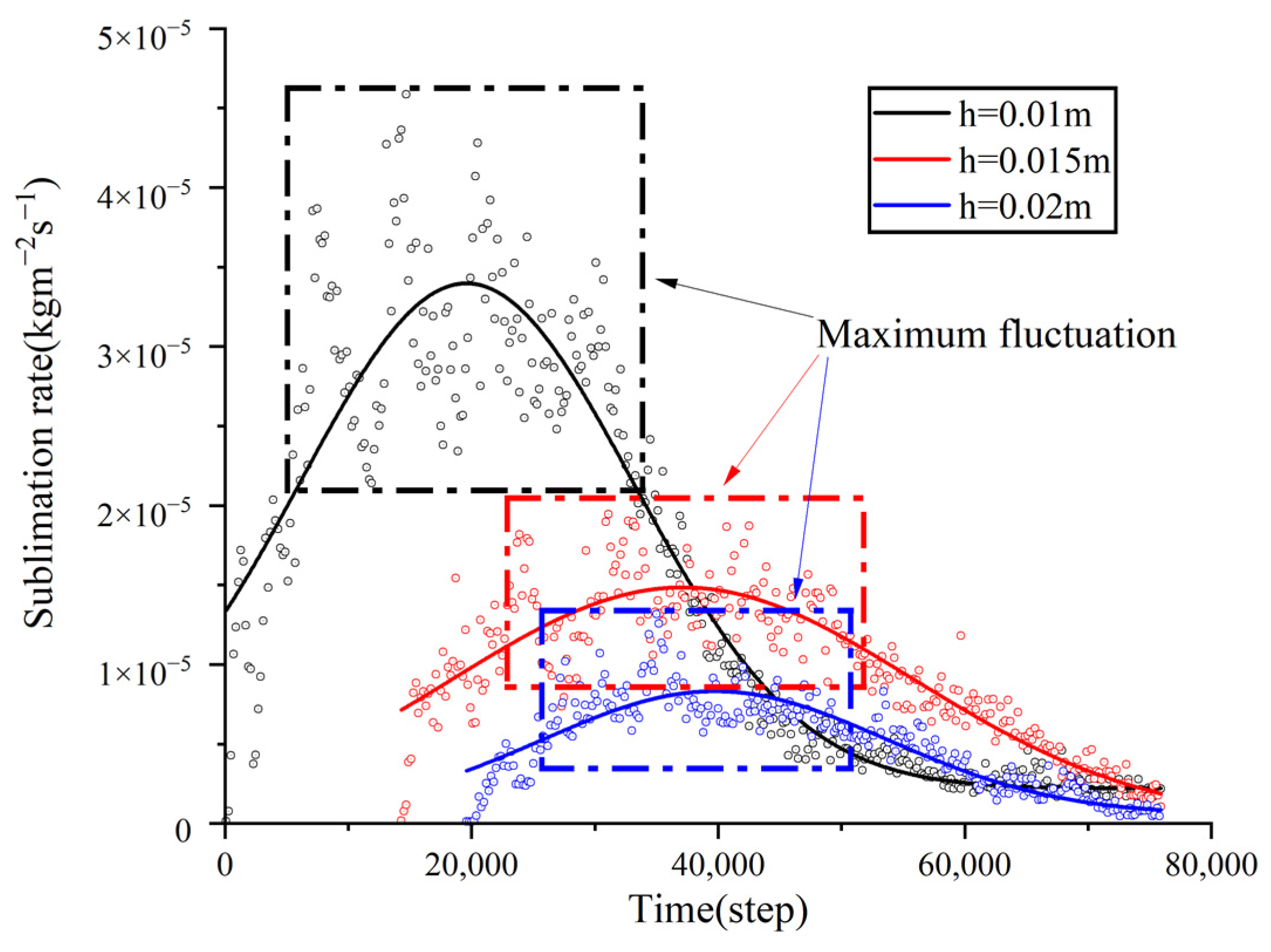
Figure 12 shows the time evolution of the sublimation rate at h = 0.01 m, h = 0.015 m, and h = 0.02 m under friction wind speed ms−1. The overall quantity of sublimation reduces with the rise in height, whereas the sublimation rate increases initially and eventually declines. This is due to the fact that when snow particles in the air increase, so does the sublimation rate. Particle number density is an important factor affecting the total sublimation rate, which is consistent with the experimental conclusion of Wever et al. (2009) [19].

Figure 12.
Time evolution of sublimation rate.
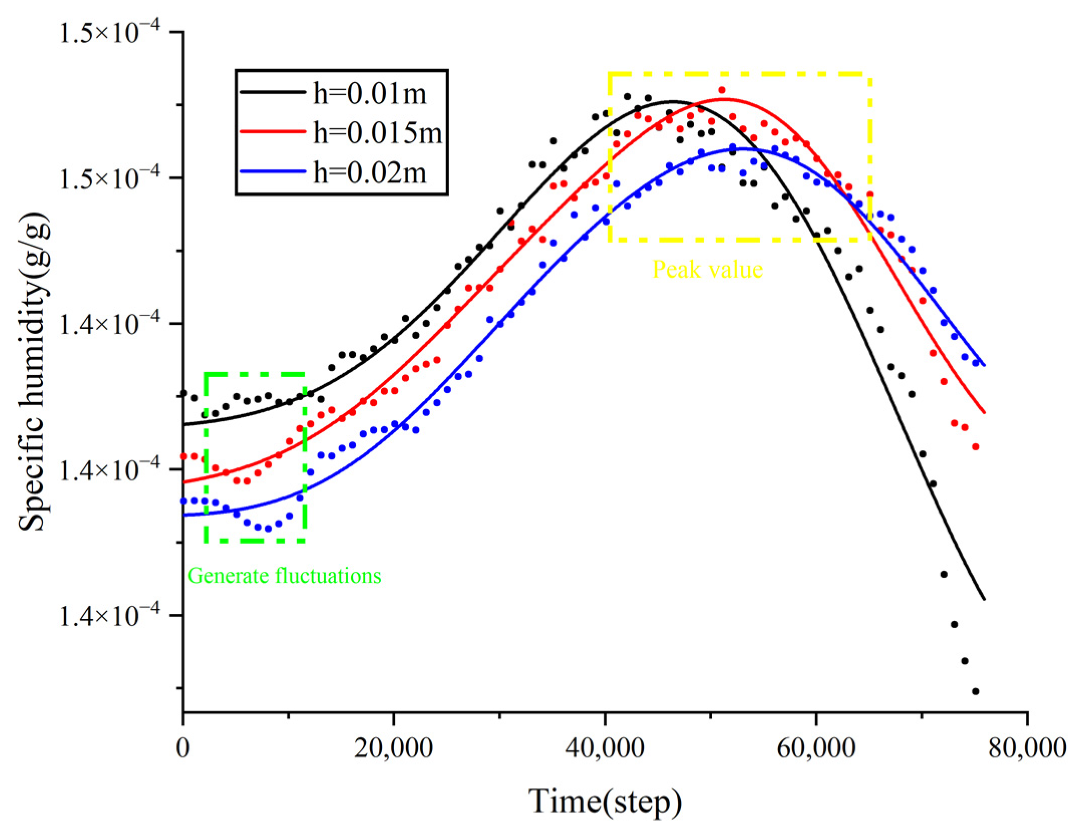
Figure 13 shows the time evolution of specific humidity at different heights. The specific humidity change is divided into the rising and falling stages. In the rising stage, the air’s water vapor content is affected by humidity, as can be seen from Figure 11b; when Step = 5000 to Step = 10,000, both humidity and specific humidity show the same regular fluctuation phenomenon. At the same time, the specific humidity and humidity increase with the increase in height. In the falling stage, the air’s water vapor content is affected by temperature. This is because the specific humidity increases with the increase in height, opposite to the rising stage. It can be seen from Figure 11c that the temperature increases with the increase in height, which is the same as the change rule of specific humidity. This is because the air humidity is stable at this time, and the temperature continues to decrease, which leads to a continuous decrease in saturated water vapor pressure.

Figure 13.
Time evolution of specific humidity.
The distribution of snow particle velocity, mass flux, and particle size verified the accuracy and feasibility of the wind-blown snow motion model. The accuracy and feasibility of the SPH method to simulate snow-blowing sublimation were verified by the sublimation rate, temperature, and humidity variation.
5.2. Simulation Analysis of Embankment and Cutting
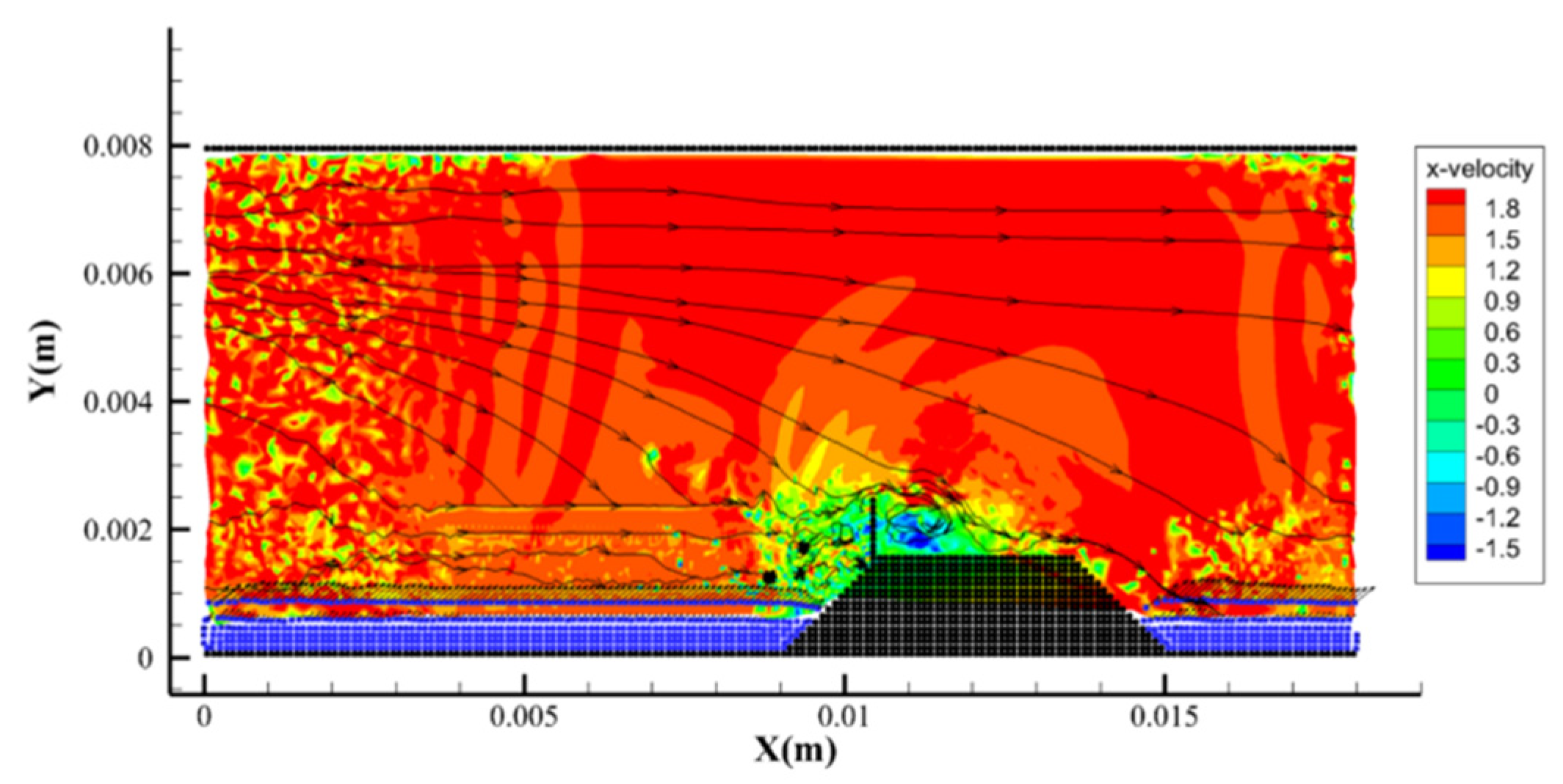
Figure 14 and Figure 15 are the streamlines of embankment and cutting when Step = 1400, respectively. The velocities around the embankment and cutting have different changes, and the distribution characteristics of the whole flow field are changed due to their existence. The upwind slope of the cutting forms a vortex.
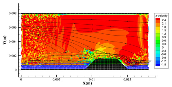
Figure 14.
Embankment model—Streamline diagram of velocity.
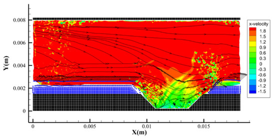
Figure 15.
Cutting model—Streamline diagram of velocity.
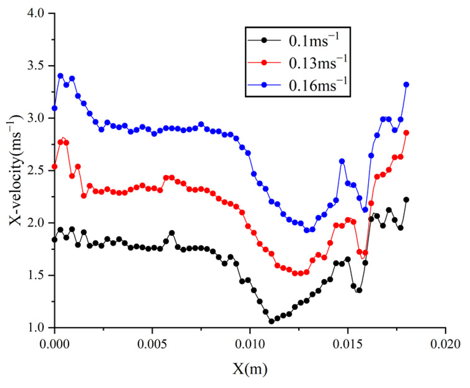
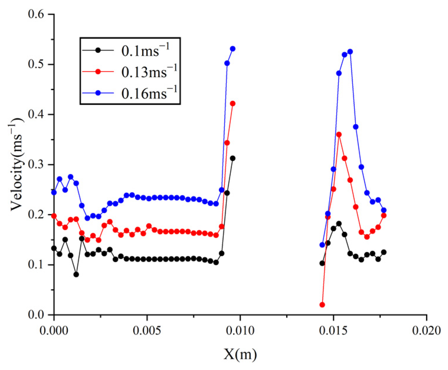
Figure 16 and Figure 17 are the distribution characteristics of the horizontal velocity of air particles. The horizontal velocity of the windward slope of the embankment changes the most under different frictional wind speeds, which is due to the blocking effect of the embankment itself. For the cutting, due to the formation of convective wind, the wind speed at the subgrade surface is the smallest.
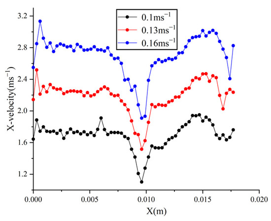
Figure 16.
Embankment model—horizontal air velocity.

Figure 17.
Cutting model—horizontal air velocity.
Due to the action of the airflow, the snow particles obtain a certain take-off speed, but the speed of the snow particles near the embankment and the cutting changes abruptly, as shown in Figure 18 and Figure 19. This is due to the disorder of the air around the cutting and embankment, resulting in frequent collisions of snow particles and increasing kinetic energy.

Figure 18.
Embankment model—the take-off speed of snow particles.
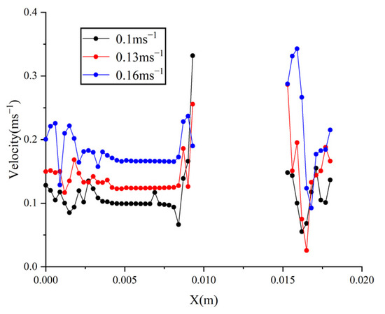
Figure 19.
Cutting model—the take-off speed of snow particles.
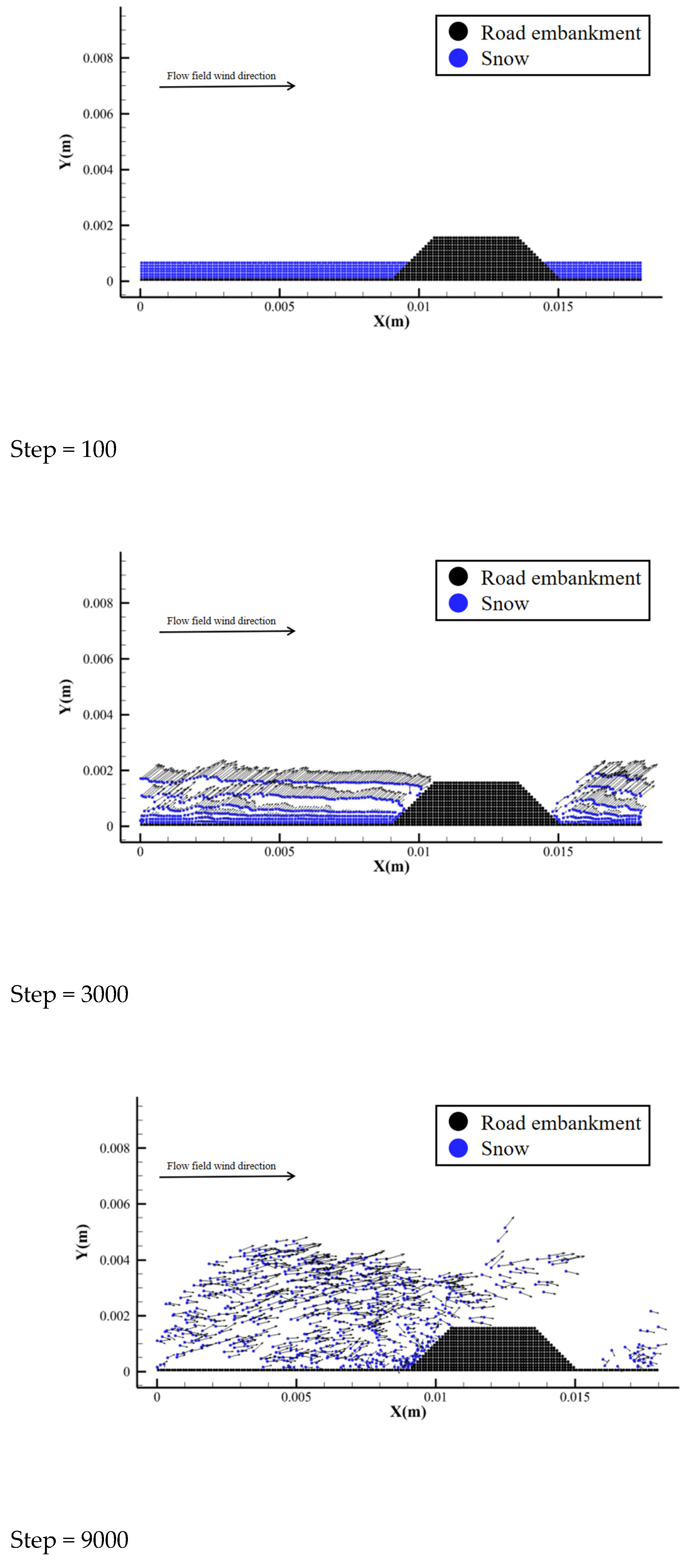
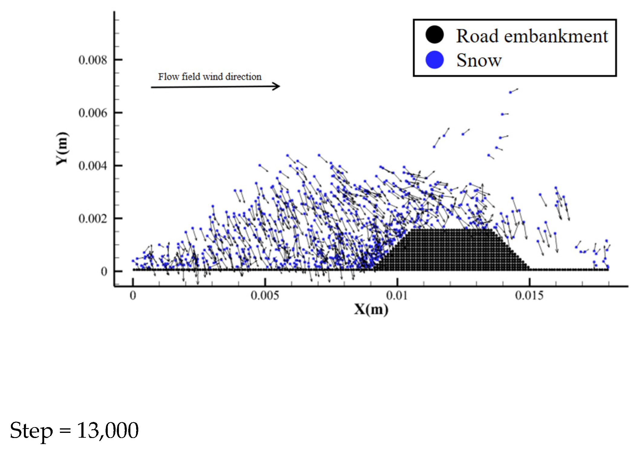
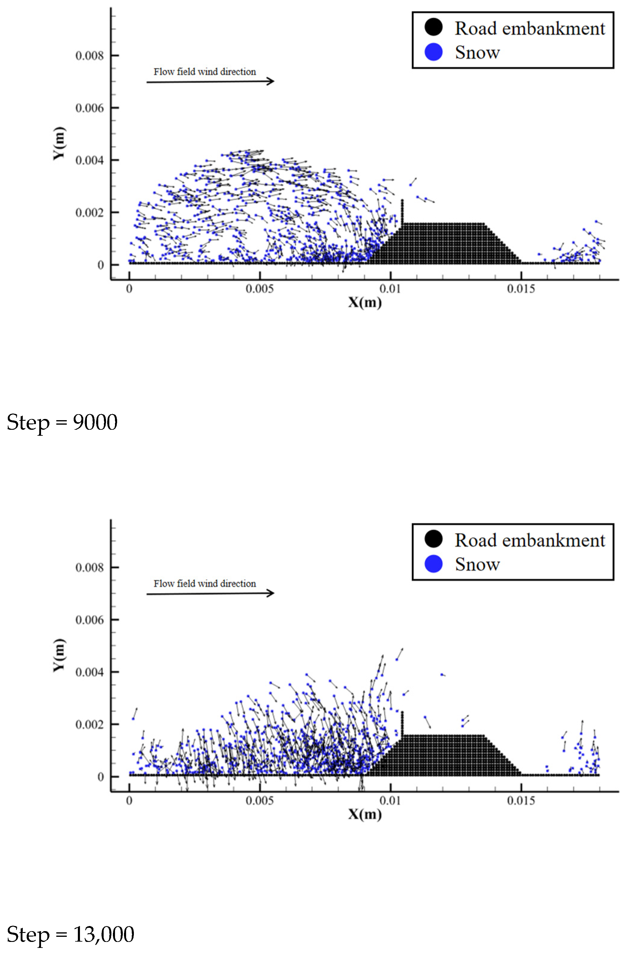
Figure 20 is the embankment model for the space–time distribution of snow particles. The saltation movement of snow grains goes through three stages: starting, developing, and falling, corresponding to Step = 3000, Step = 9000, and Step = 13,000, respectively. In the start-up phase, the snow particles obtain a certain take-off speed, and the reasons for the flow field, the size, and the direction of the speed are different. In the development stage, the vertical velocity of most snow particles is zero, showing a horizontal motion state, and some snow particles leap to the embankment. In the falling stage, most of the snow particles complete a jump movement. The damage to traffic is divided into falling on the subgrade surface and leaping over the subgrade, which may cause vehicle skidding, derailment, and reduced visual range.
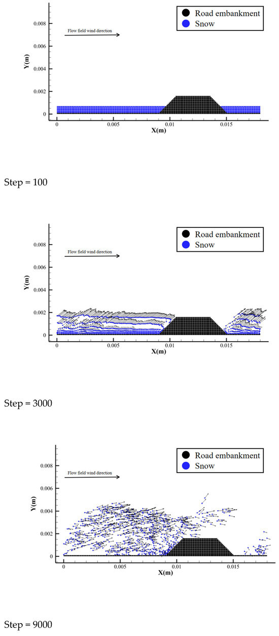
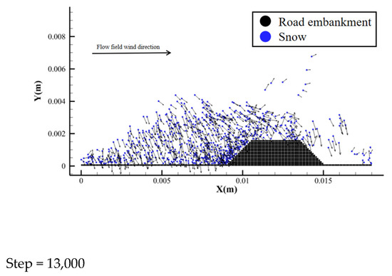
Figure 20.
Embankment model—snow temporal and spatial distribution map.
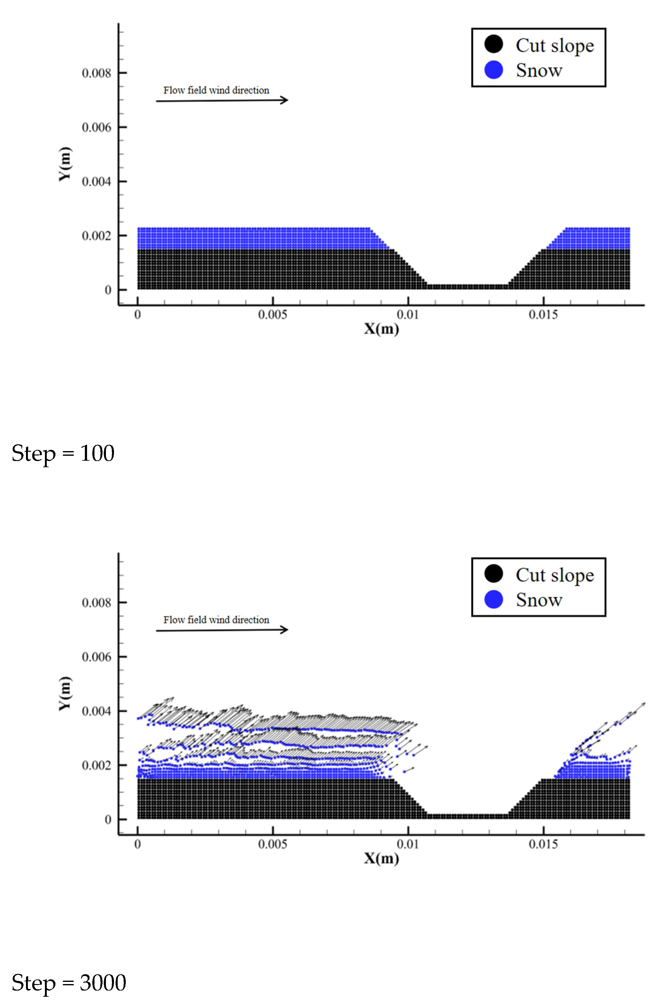
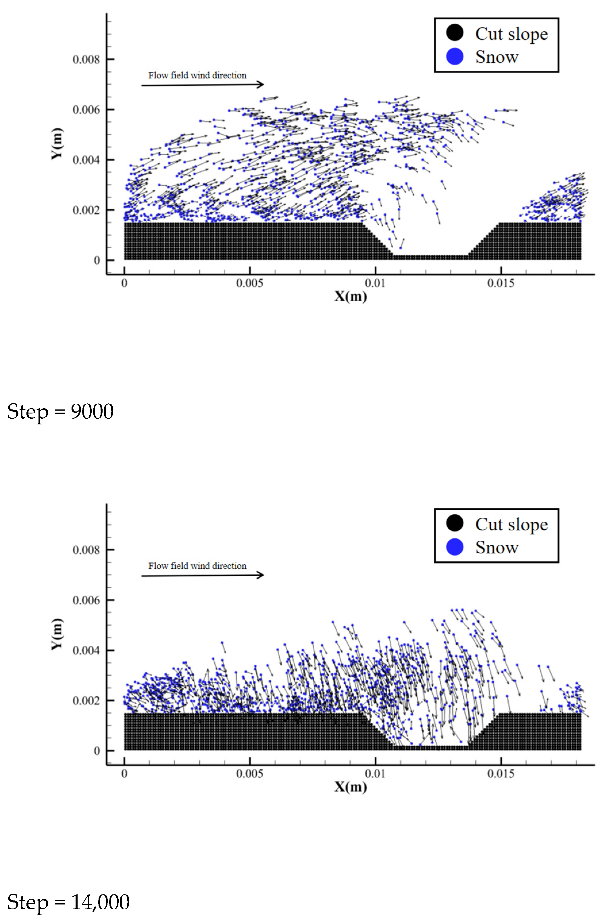
Figure 21 is the cutting model for the snow grain space–time distribution. The three stages of snow movement correspond to Step = 3000, Step = 9000, and Step = 14,000. Due to the low terrain of the cutting, there is no advantage that the embankment itself can block, so more snow particles enter the cutting, and the wind and snow disasters in the cutting are more serious.
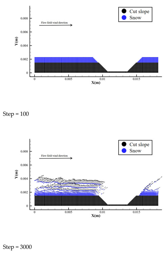
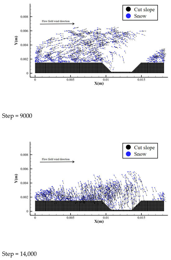
Figure 21.
Cutting model—spatiotemporal distribution of snow grains.
5.3. Analysis of Causes of Snow Disaster
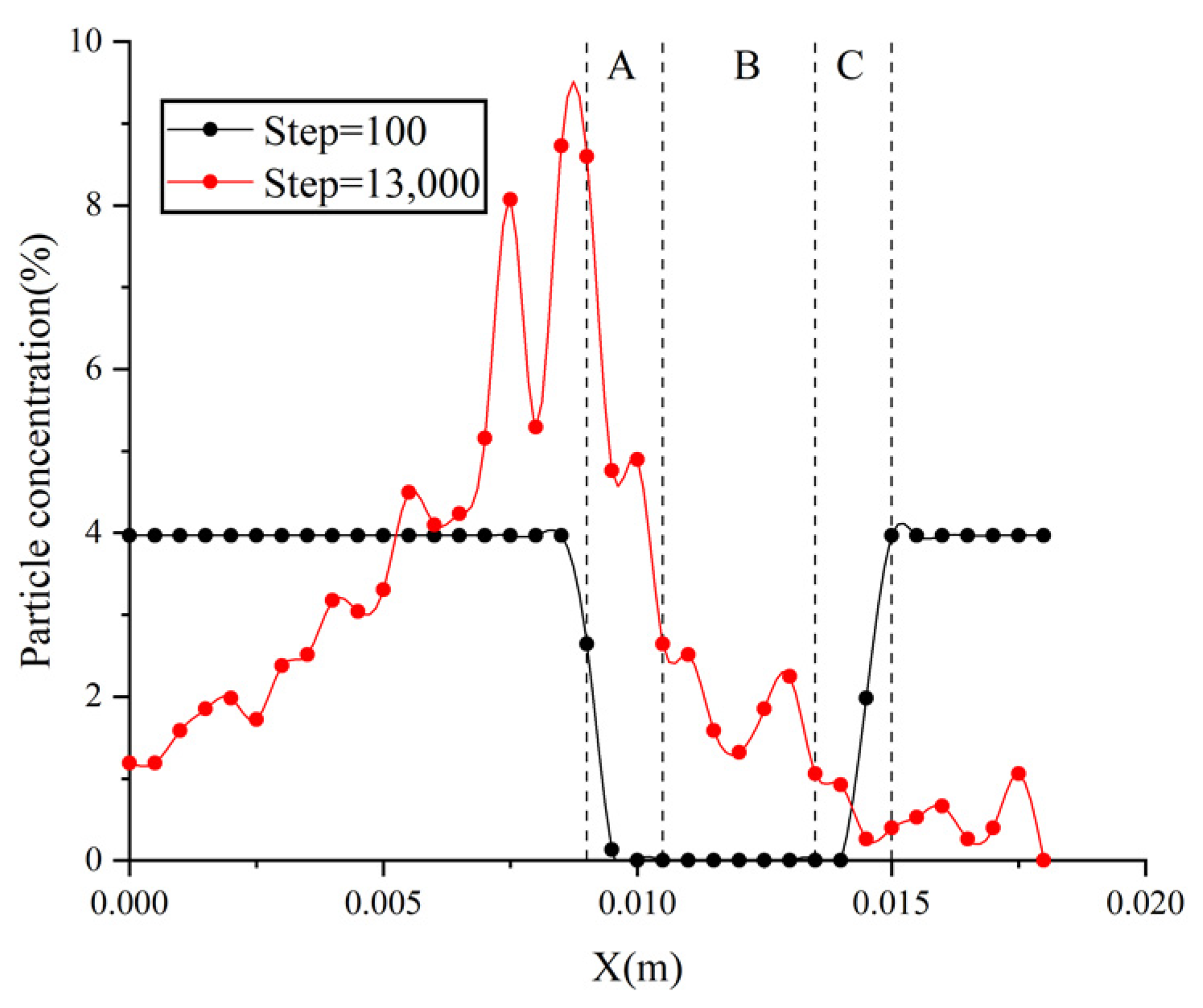
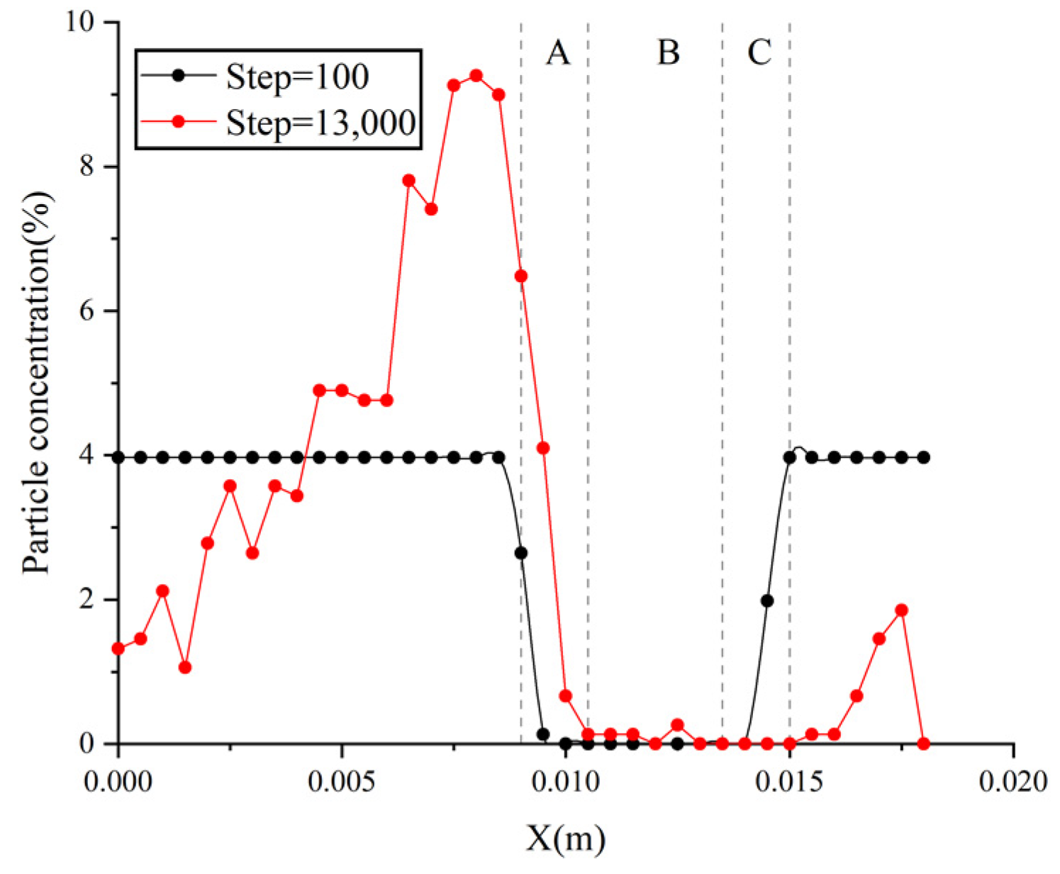
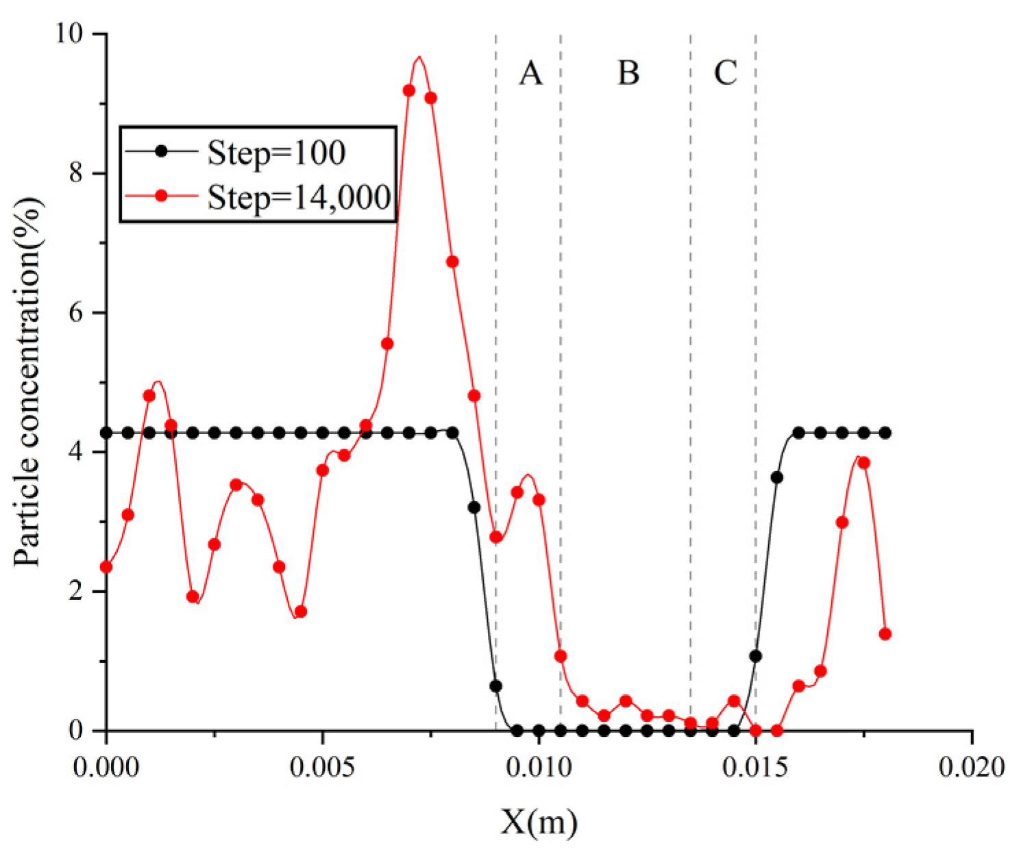
Figure 22 shows the snow particle concentration distribution in regard to the distribution law of the embankment model. When Step = 100, the snow particles hardly move, and the snow particle concentration is evenly distributed. In the falling stage of Step = 13,000 embankment, the peak value of the snow concentration is before the windward slope of the embankment, which is due to the height of the embankment itself.
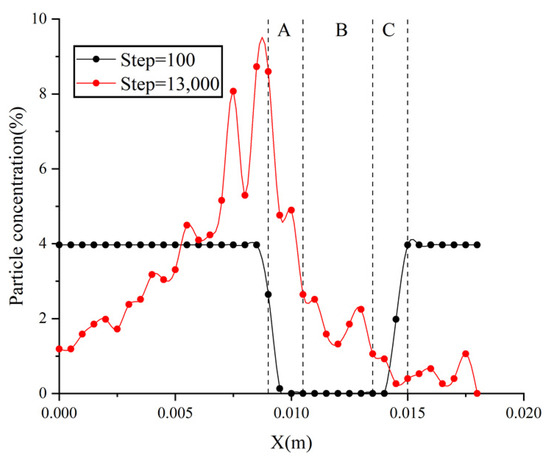
Figure 22.
Embankment model—snow particle concentration distribution.
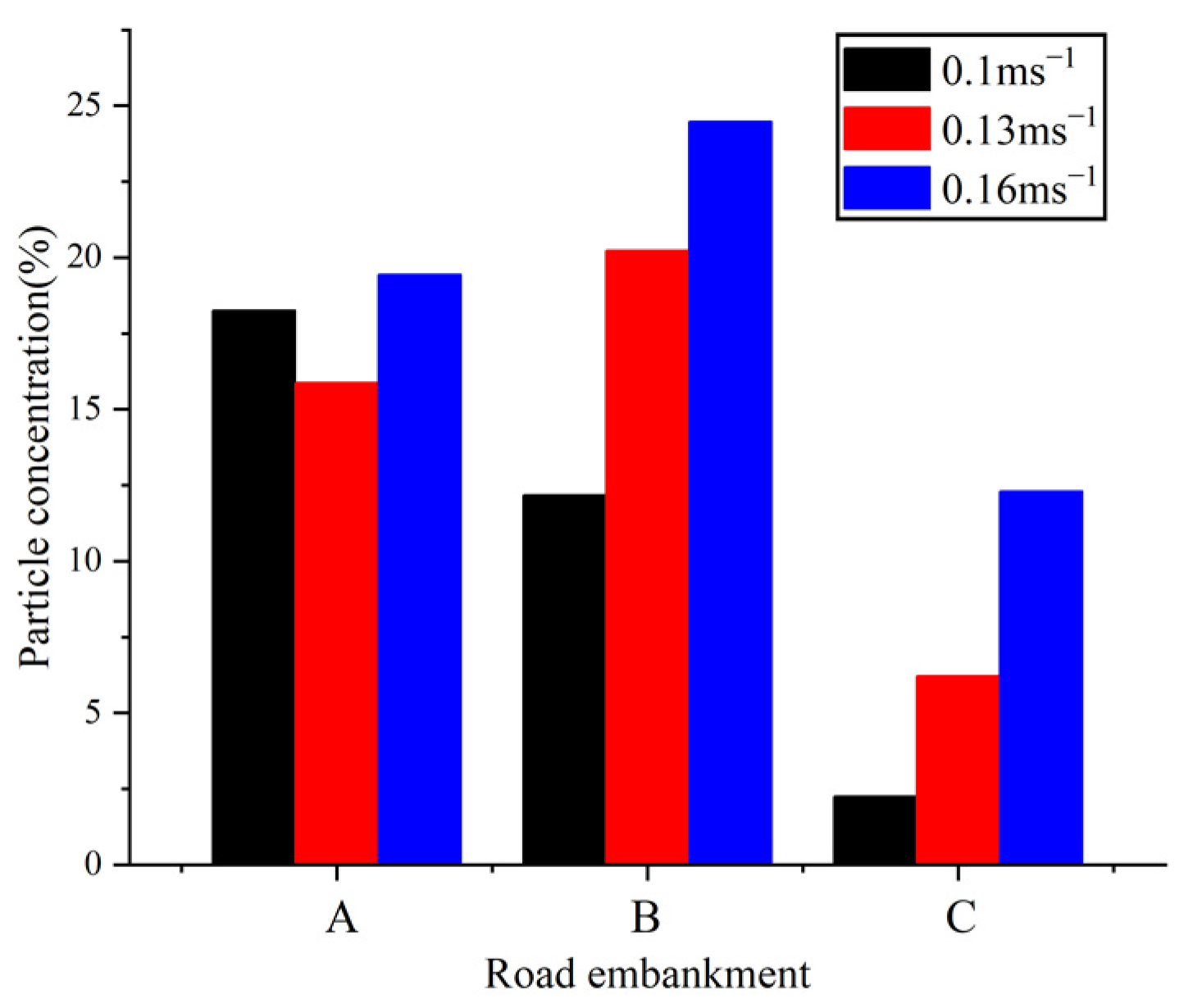
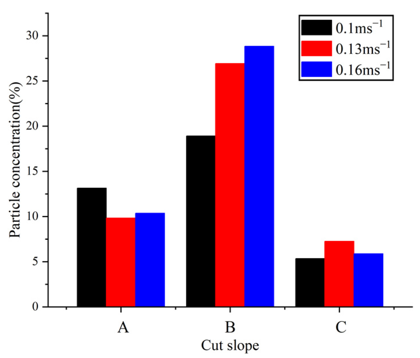
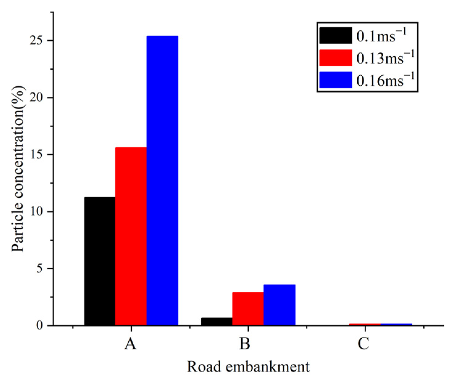
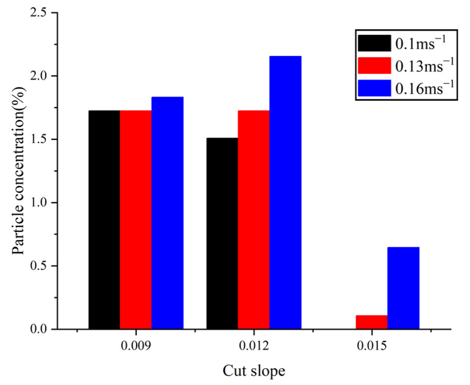
Figure 23 shows the snow burial ratio in regard to the distribution law of the embankment model. The research is focused on region B, where driving occurs, and reveals that the amount of snow particles increases when the friction wind speed rises. The snow particles that fall on the embankment are mostly dispersed in areas A and B. This is because the greater the friction wind speed, the more kinetic energy the snow particles obtain and the higher the take-off height.
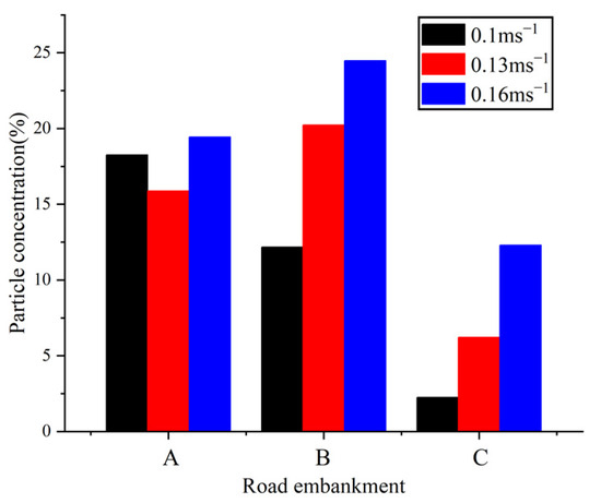
Figure 23.
Embankment model—snow burial ratio.
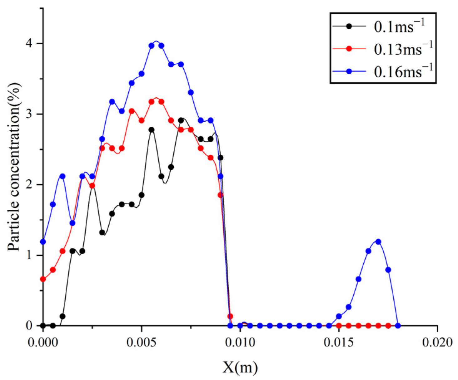
Figure 24 shows the source distribution of snow particles on the embankment. The snow particles that cause danger to the embankment mainly come from 0.004 m to 0.008 m, and the range increases with the increase in friction wind speed. This part of the snow is little affected by the embankment, and there is enough energy to reach the embankment.

Figure 24.
Embankment model—snow source distribution.
Through the analysis of Figure 22, Figure 23 and Figure 24, it can be ascertained that the embankment itself can block some snow particles, but due to the height, some snow particles still have enough kinetic energy to reach the subgrade surface, and these snow particles are less affected by the embankment. Through the above, it can be concluded that increasing the height of the embankment can effectively reduce the transport of snow particles, and this effect can be achieved by establishing a snow fence.
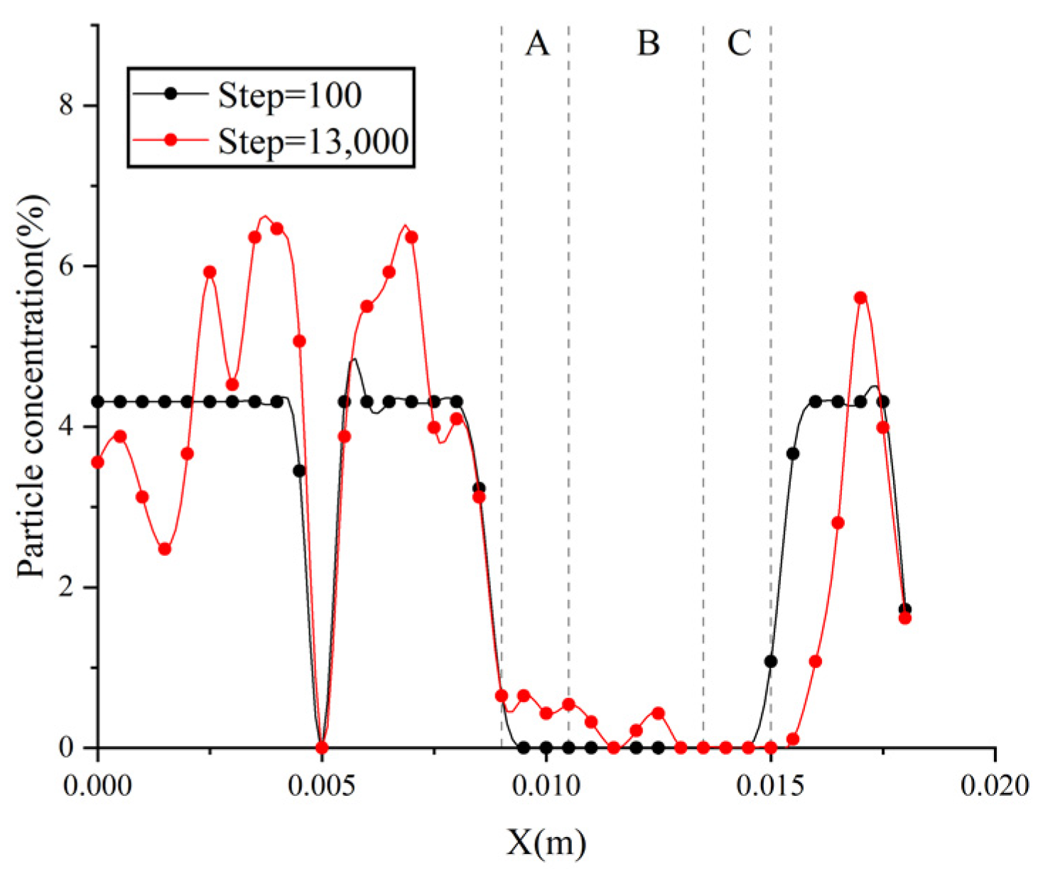
As shown in Figure 25, presenting the cutting model for snow particle concentration distribution, when Step = 100, the snow particle concentration is evenly distributed. In the falling stage, the peak value of snow particle concentration is on the upwind slope of the cutting, which is due to the low altitude of the cutting, so most of the snow particles will move to the cutting. As shown in Figure 26, presenting the distribution of the cutting model’s snow burial ratio, most of the snow particles falling on the cutting are on the subgrade surface, which is because the snow particles are not blocked from obtaining more energy, and the slopes on both sides of the cutting are more conducive to the downward movement of the snow particles.
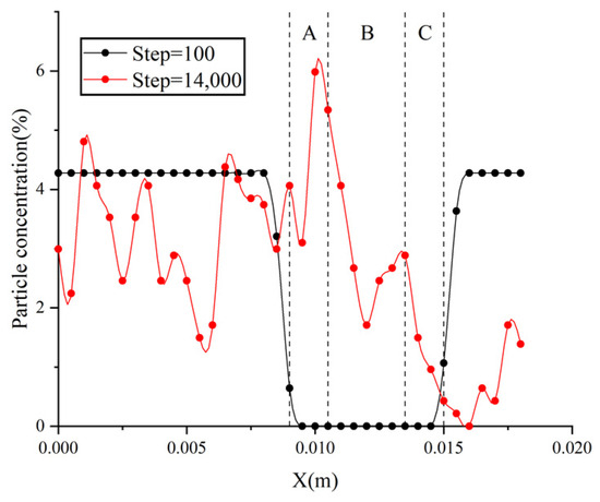
Figure 25.
Cutting model—snow particle concentration distribution.

Figure 26.
Cutting model—snow burial ratio.
As shown in Figure 27, presenting the cutting model for snow source distribution, due to the terrain, the dangerous snow particles on the cutting mainly come from before 0.009 m and decrease with the increase in the distance from the cutting. Because the kinetic energy obtained by the farther snow particles is insufficient to move to the cutting, the snow particles in the cutting mainly come from before the upwind slope.
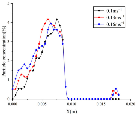
Figure 27.
Cutting model—snow source distribution.
Through the analysis of Figure 25, Figure 26 and Figure 27, it can be ascertained that most of the snow particles can move to the subgrade surface due to the shortcomings of the cutting structure, and these are mainly snow particles closer to the cutting. Therefore, through the above conclusions, we can surmise that the snow fence can be added to the windward slope to change the wind speed of the flow field so that the snow particles in the area can obtain less energy.
5.4. The Results of Adding a Snow Fence
Through a series of analyses of the particle concentration distribution, snow burial ratio, and snow particle source of the embankment and cutting model, a snow-proof structure suitable for different working conditions was designed. Extending the advantages of the height of the embankment model, an anti-snow fence was erected at the junction of the windward slope and the subgrade surface. For the cutting, the anti-snow fence with a forward tilt of about 45 degrees was most beneficial, to reduce the snow concentration in the cutting (Li, 2021 [18]).
Figure 28 shows the snow grain spatial and temporal distribution for the anti-snow fence model of the embankment. It can be found from the figure that only a small portion of the snow particles crossed the snow fence, while most of the snow particles were blocked in front of the snow fence. The peak concentration of snow particles was near 0.008 m, and there were very few snow particles that could reach the subgrade surface, as shown in Figure 29. Therefore, for the embankment, adding the snow fence can do well to block the leap of snow. The anti-snow fence blocks the flow rate of air at low altitudes, which decreases the momentum obtained by snow particles, and there is insufficient momentum to leap over the anti-snow fence.
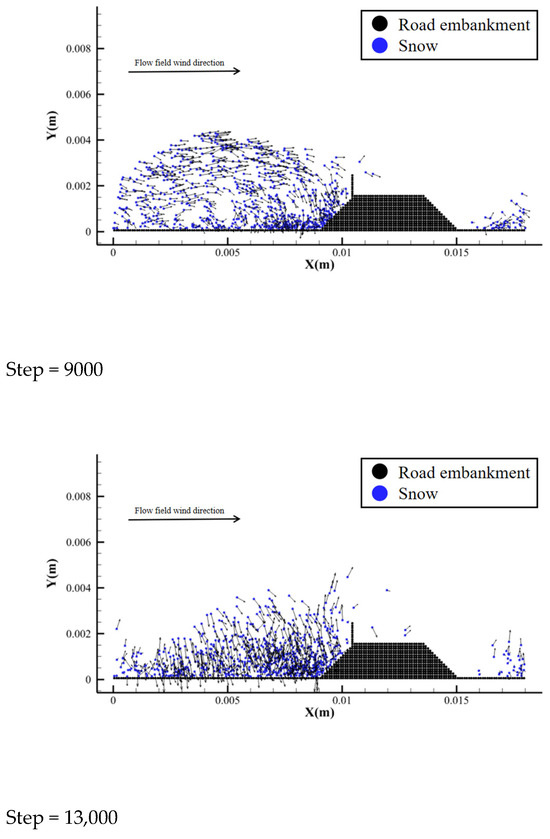
Figure 28.
Anti-snow fence model of embankment—snow grain space–time distribution map.
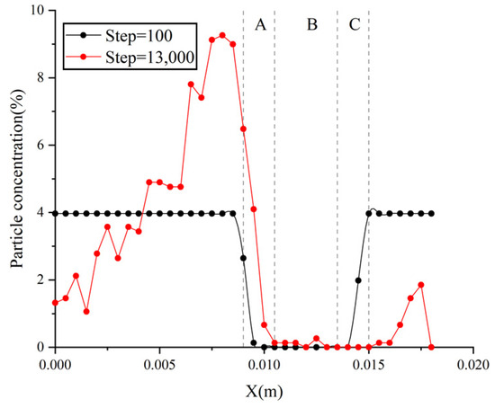
Figure 29.
Anti-snow fence model of embankment—snow particle concentration distribution.
Figure 30 shows the snow burial ratio for the anti-snow fence model of the embankment. While the snow particles on the windward slope rise noticeably, the snow particles on the embankment increase as friction increases. This is because the snow particles obtain more energy, and the farther snow particles move to the vicinity of the embankment. However, the existence of the anti-snow fence blocks the snow particles from moving closer.

Figure 30.
Anti-snow fence model of embankment—snow buried ratio.
Table 2 is snow reduction ratio change for the embankment snow fence model. The proportion of snow particles on the embankment decreases with the increase in friction wind speed, and the reduction in all working conditions reaches about 50%, which also shows that the establishment of a snow fence reduces the erosion of snow particles on the embankment. The snow amount on the subgrade surface is reduced by more than 85%, and the snow amount on the leeward slope is reduced by 97%. Therefore, the establishment of this anti-snow fence can do well to prevent wind-blown snow disasters under these conditions.
Table 2.
Anti-snow fence model of the embankment—snow reduction ratio change.
As shown in Figure 31, presenting the snow grain space–time distribution for the cutting anti-snow fence model, the forward-tilting 45-degree snow fence blocked the movement of nearby snow particles, but the blocking effect on distant snow particles gradually decreased, so some snow particles leaped to the subgrade surface. Although the peak value of snow particle concentration changed to about 0.008 m, there were still some snow particles on the cutting, as shown in Figure 32. The impact of snow prevention was also noticeably diminished for the snow fence of the cutting model when the friction wind speed increased, as illustrated in Figure 33.
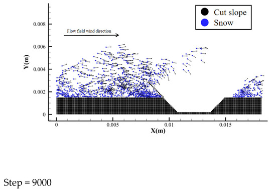
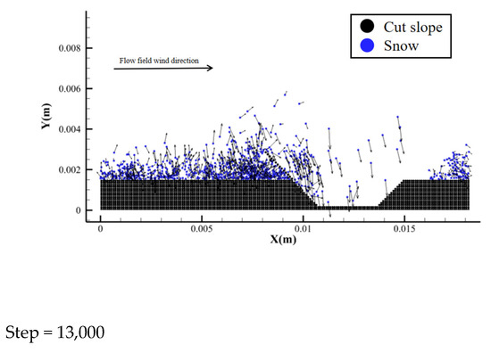
Figure 31.
Cutting anti-snow fence model—snow grain space–time distribution map.
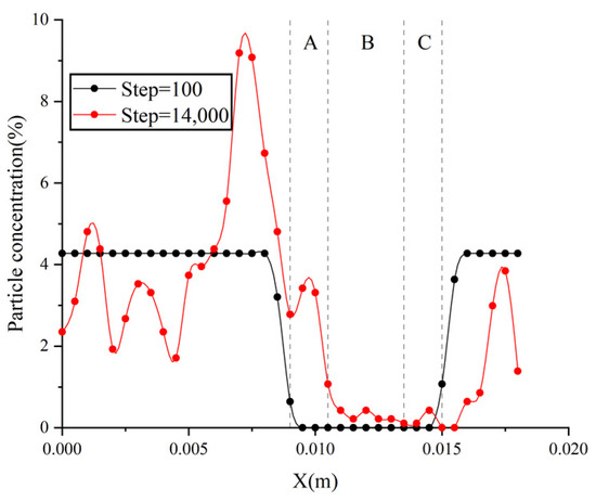
Figure 32.
Anti-snow fence model of cutting—snow particle concentration distribution.
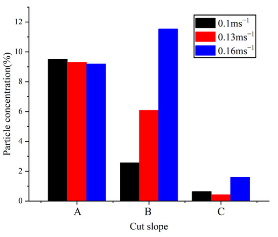
Figure 33.
Anti-snow fence model of cutting—snow buried ratio.
Table 3 is the cutting anti-snow grille model for snow reduction ratio change. The total amount of snow particles in the cutting is reduced with the increase in friction wind speed, and the reduction is more than 50%. Therefore, the addition of a snow fence reduces the erosion of snow particles on the cutting. However, the proportion of snow reduction on the subgrade surface decreases with the increase in friction wind speed, and the effect of snow prevention gradually weakens. Therefore, under the circumstance of high friction wind speed, the front 45-degree anti-snow grille cannot adequately satisfy the operating circumstances of the cutting model.
Table 3.
Anti-snow fence model of the cutting—change in snow reduction ratio.
Figure 34 presents a flow diagram of the road embankment snow fence model. The construction of a snow fence causes the flow field around the subgrade to change greatly. The windward side of the snow fence collides with the incoming wind, and the air in the area becomes disarranged. On the leeward side, negative pressure areas are formed, creating a pronounced vortex. The change in flow field and the relative increase in height can effectively prevent the erosion of the embankment by the storm disaster.
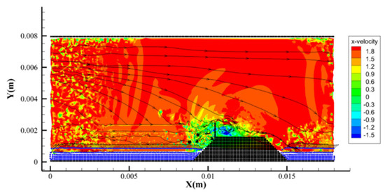
Figure 34.
Anti-snow fence model of embankment—Streamline diagram of velocity.
5.5. The Results of Increasing the Snow Fences
Because the forward-tilting 45-degree snow fence could not meet the working conditions of the cutting model well, we sought to identify the source of dangerous snow particles. We found that the snow particles on the cutting were mainly from the vicinity (within 0.005 m), as shown in Figure 35. Therefore, according to the above data, a vertical anti-snow fence was added near 0.005 m to scramble the flow field wind speed in this area and reduce the kinetic energy obtained by snow particles, thus effectively preventing the take-off of snow particles.
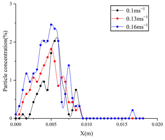
Figure 35.
Anti-snow fence model of cutting—snow source distribution.
As shown in Figure 36, containing the snow grain space–time distribution for multiple anti-snow fence models of cutting, the speed and number of snow particles that take off near the snow fence are significantly lower, while the energy obtained by the snow particles near 0.005 m is obviously insufficient for the snow particles to move to the cutting. Due to the change in the surrounding flow field caused by the snow fence, the kinetic energy of the snow particles is reduced, and the distance of their movement is reduced.
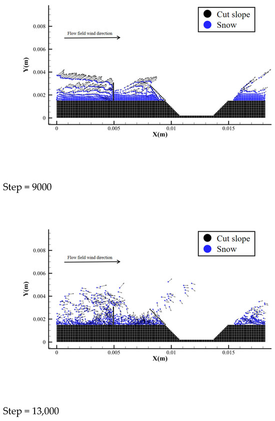
Figure 36.
Multiple anti-snow fence models of cutting—snow grain space–time distribution map.
As shown in Figure 37, containing the snow particle concentration distribution for multiple anti-snow fence models of cutting, the impact of several anti-snow fences is substantially larger than that of a single anti-snow fence, and the two peaks of the snow particle concentration occur at the sites of the anti-snow fences. Only a small portion of the snow particles move to the cutting. Although the number of snow particles on the subgrade surface of the cutting increases with the increase in the friction wind speed, the degree of increase is significantly lower than the effect of a single snow fence, as shown in Figure 38.
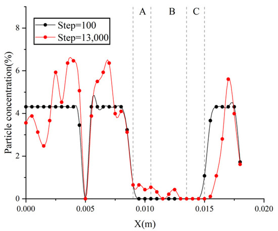
Figure 37.
Multiple anti-snow fence models of cutting—snow particle concentration distribution.
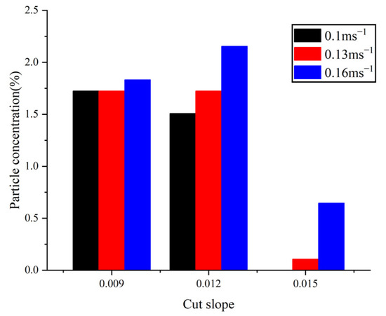
Figure 38.
Multiple anti-snow fence models of cutting—snow buried ratio.
Through the results presented in Table 4, we found that occurrences of snow on the whole cutting decreased by about 90%, while the number of snow particles on the subgrade surface decreased by about 93%. This further shows that multiple anti-snow fences can effectively prevent the movement of snow particles and the rationality of installing the anti-snow fence position.
Table 4.
Multi-snow-fence model of the cutting change in snow reduction ratio.
6. Conclusions
This paper has presented a wind and snow disaster simulation software based on the smooth particle hydrodynamics (SPH) method, which will avoid the blindness of traditional wind and snow disaster management, reduce the process of continuous testing in the middle, and achieve targeted treatment of wind and snow disasters. Compared with the traditional SPH particle modeling method, the pixel value method proposed in this paper is faster and more accurate in the establishment of boundary particles and can be well-adapted to the establishment of various complex 2D models.
The feasibility of the snow flow motion model was verified using the snow particle velocity, the uppermost snow particle motion position and velocity change, mass flux, and average particle size distribution. The validity of the sublimation model was verified via the sublimation of air temperature, air relative humidity, air specific humidity, and snow particles. The results demonstrate the SPH method’s significant benefits in the control of wind and snow catastrophes. The following conclusions were drawn in this study:
- In the start-up phase, the uppermost snow particles obtain almost the same speed under the influence of air drag force. The size and direction of snow particle velocity in the same layer change significantly over time. The pace at which snowflakes sublimate likewise alters as a result of this alteration. The SPH approach yielded a velocity probability distribution of snow particles that is consistent with the earlier experimental findings.
- The sublimation rates at different heights showed a trend of increasing first and then decreasing. Although the temperature and humidity at the low altitude changed significantly, which led to a significant increase in the negative feedback effect, the total sublimation amount showed the opposite trend with the increase in height due to the large particle density of sublimated snow particles. Before humidity stabilizes, it is the most important factor affecting the specific humidity. However, temperature is the primary factor impacting a given humidity level when the humidity is steady.
- Through the SPH simulation software established in this paper, targeted snow and sand prevention was implemented for typical embankment and cutting conditions of wind and snow disasters. Combined with the advantages of the structure of the embankment itself, the establishment of a vertical snow fence can achieve a good snow prevention effect, and the reduction in snow on the subgrade surface can reach more than 85%. For the forward-tilting 45-degree snow fence, the snow prevention effect on the subgrade surface of the cutting is significantly reduced as the friction wind speed increases, and the smallest effect is 30.59% prevention. For the condition of multiple snow fences in the cutting, the snow-proof effect of the subgrade surface reaches about 93%. For different working conditions, different preventive measures can be taken, and our contribution reduces the blindness when experimenting with those measures.
Author Contributions
Conceptualization, S.Z.; methodology, S.Z.; software, B.Z.; formal analysis, H.P.; investigation, H.P.; data curation, H.P. and S.Z.; writing—original draft preparation, S.Z.; writing—review and editing, S.Z. and H.P.; visualization, B.Z.; supervision, A.J.; project administration, A.J. All authors have read and agreed to the published version of the manuscript.
Funding
This research was funded by National Natural Sciences Foundation of China, Grant/Award Number: 11662019.
Institutional Review Board Statement
Not applicable.
Informed Consent Statement
Not applicable.
Data Availability Statement
No new data were created or analyzed in this study. Data sharing is not applicable to this article.
Acknowledgments
The authors would like to thank the anonymous reviewers and the editor for providing valuable comments that helped improve the quality of this paper.
Conflicts of Interest
The authors declare no conflict of interest.
References
- Wang, Z.L. Research on prevention of snow damages in China. Mt. Res. 1983, 1, 22–31. [Google Scholar]
- Oki, T.; Kanae, S. Global hydrological cycles and world water resources. Science 2006, 313, 1068–1072. [Google Scholar] [CrossRef] [PubMed]
- Huang, N.; Li, G. Mountain snow: The source of the mother river-Study of multi-scale and multi-physical process of spatio-temporal evolution of snow distribution. Sci. Technol. Rev. 2020, 38, 10–22. [Google Scholar]
- Guo, S.H.; Chen, R.H.; Han, C.T. Advances in the Measurement and Calculation Results and influencing Factors of the Sublimation of lce and Snow. Adv. Earth Sci. 2017, 32, 1204–1217. [Google Scholar]
- Han, K. A Numerical Simulation on the Development Process of Blowing Snow and the Effects of Snow Grains. Master’s Thesis, Lanzhou University, Lanzhou, China, 2007. [Google Scholar]
- Wever, N.; Lehning, M.; Clifton, A.; Rüedi, J.-D.; Nishimura, K.; Nemoto, M.; Yamaguchi, S.; Sato, A. Verification of moisture budgets during drifting snow conditions in a cold wind tunnel. Water Resour. 2009, 45, W07423. [Google Scholar] [CrossRef]
- Hung, N.; Shi, G.L. The significance of vertical moisture diffusion on drifting snow sublimation near snow surface. Cryosphere 2017, 11, 3011–3021. [Google Scholar] [CrossRef]
- An, Z.; Jin, A.; Musa, R. SPH numerical simulation study on wind-sand flow structure of multi-diameter sand. Comp. Part. Mech. 2022, 10, 747–756. [Google Scholar] [CrossRef]
- Bintanja, R. The contribution of snowdrift sublimation to the surface mass balance of Antarctica. Ann. Glaciol. 1998, 27, 251–259. [Google Scholar] [CrossRef]
- Hung, N.; Dai, X.Q. The impacts of moisture transport on drifting snow sublimation in the saltation layer. Atmos. Chem. Phys. 2016, 16, 7523–7529. [Google Scholar] [CrossRef]
- Shi, G.L. A General Model of Blowing Snow:Saltation and Suspension. Ph.D. Thesis, Lanzhou University, Lanzhou, China, 2018. [Google Scholar]
- Zhang, S.C. Smoothed particle hydrodynamics (SPH) method (a review). Chin. J. Comput. Phys. 1996, 4, 2–14. [Google Scholar]
- Jin, A.F.; Ayni, M.M.T.M. SPH-based numerical calculation of sand grain velocity distribution in wind-blown sand flow. Arid. Zone Res. 2018, 35, 107–113. [Google Scholar]
- Li, D.C.; Guang, X.; Sun, Z.G. Uniform discretization of 2-dimensional complex geometrical area for meshless particle Method. J. Xi’an Jiaotong Univ. 2013, 47, 120–126. [Google Scholar]
- Jin, A.F.; Gheni, M.; Yang, Z.C. Numerical Simulation of Sand Cover Phenomenon on the Desert Highway Using SPH Method. Adv. Mater. Res. 2018, 33, 1075–1082. [Google Scholar] [CrossRef]
- Thorpe, A.D.; Mason, B.J. The evaporation of ice spheres and ice crystals. Br. J. Appl. Phys. 1966, 17, 541–548. [Google Scholar] [CrossRef]
- Bintanja, R. Snowdrift suspension and atmospheric turbulence, Part I: Theoretical background and model description. Bound.-Layer Meteorol. 2000, 95, 343–368. [Google Scholar] [CrossRef]
- Li, H.F.; He, S.Y.; Liu, Q.K. Numerical study on the influence of slope and snow-fence on the flow field around embankment. Eng. Mech. 2021, 38, 21–25. [Google Scholar]
- Lv, X.H. Some Investigations into Wind Snow Two Phase Flow in Wind Tunnel. Ph.D. Thesis, Lanzhou University, Lanzhou, China, 2012. [Google Scholar]
- Li, F.Q. Research on Profiles of Blowing Snow and Snow Distribution on Traffic Line. Master’s Thesis, Shijiazhuang Tiedao University, Shijiazhuang, China, 2021. [Google Scholar]
- Sugiura, K.; Nishimura, K.; Maeno, N.; Kimura, T. Measurements of snow mass flux and transport rate at different particle diameters in drifting snow. Cold Reg. Sci. Technol. 1998, 27, 83–89. [Google Scholar] [CrossRef]
- Dover, S.E. Numerical Modelling of Blowing Snow. Ph.D. Thesis, University of Leeds Department of Applied Maths, Leeds, UK, 1993. [Google Scholar]
- Gordon, K.; Taylor, P. Measurements of blowing snow, Part I: Particle shape, size distribution, velocity, and number flux at Churchill, Manitoba, Canada. Cold Reg. Sci. Technol. 2009, 55, 63–74. [Google Scholar] [CrossRef]


Disclaimer/Publisher’s Note: The statements, opinions and data contained in all publications are solely those of the individual author(s) and contributor(s) and not of MDPI and/or the editor(s). MDPI and/or the editor(s) disclaim responsibility for any injury to people or property resulting from any ideas, methods, instructions or products referred to in the content. |
© 2023 by the authors. Licensee MDPI, Basel, Switzerland. This article is an open access article distributed under the terms and conditions of the Creative Commons Attribution (CC BY) license (https://creativecommons.org/licenses/by/4.0/).