River-Blocking Risk Analysis of the Bageduzhai Landslide Based on Static–Dynamic Simulation

Abstract

Landslides blocking rivers in alpine canyon areas can cause great harm. Taking the Bageduzhai landslide on the southeastern margin of the Qinghai-Tibet Plateau as an example, the risk of landslides blocking rivers is analyzed by static analysis and dynamic simulation. Through onsite investigation, it is found that the Bageduzhai landslide is a traction-falling landslide, and there are two sliding surfaces: deep and shallow. Through static analysis of the stability of the Bageduzhai landslide under ordinary rainfall conditions and high-intensity rainfall conditions, the sliding surface position is obtained. On this basis, the smooth particle hydrodynamics method is used to analyze the movement process and accumulation form of the landslide under different working conditions. The analysis results show that the instability volume and sliding surface depth of the landslide under ordinary rainfall conditions are significantly smaller than those under high-intensity rainfall conditions. The instability volume and sliding surface depth under ordinary rainfall conditions can reach 31 m. The river-blocking depth under extreme rainfall conditions can exceed 65 m. The research results provide theoretical support for the risk analysis of the potential river-blocking disaster of the Bageduzhai landslide.

1. Introduction

Landslides in mountainous areas are one of the most threatening geological disasters. Landslide disasters in alpine canyon areas can lead to serious river-blocking disasters and threaten the safety of upstream and downstream roads, bridges and settlements. Western Sichuan is in the southeastern margin of the Qinghai-Tibet Plateau. From east to west, there are the Minjiang River, Dadu River, Yalong River and Jinsha River. The alpine gorge area where these rivers are located has been a high-incidence area for landslide disasters since ancient times. In 1786, the Dadu River Mogangling landslide dammed the Dadu River for 9 days, and the outburst flood caused 100,000 casualties along the downstream coast. The Wenchuan earthquake in 2008 induced up to 34 large river-blocking landslides, including the Tangjiashan landslide. In 1983, the ancient Sissle landslide in the United States blocked the Falk River in Utah, forming a 78 million m³ barrier lake that flooded the town of Sissle and caused damage estimated at more than USD 200 million. In 2005, a 7.6-magnitude earthquake in Pakistan triggered a large landslide and blocked a river, forming a 130 m high barrier dam. The incident killed a total of 1000 people and completely destroyed a village. In January 2010, a landslide dam that had occurred on the Hunza River at the junction of China and Pakistan failed and destroyed the China–Pakistan Expressway, which is the highest altitude roadway in the world, and caused more than 20 deaths [1]. In November 2018, a landslide occurred again at the ‘10.11’ mountain landslide point in Baige Village, Boluo Township, Jiangda County, Changdu City, Tibet Autonomous Region, causing the Jinsha River to be blocked and a barrier lake to be formed. After the flood discharged, a large flood peak appeared due to the excessive accumulation of water. The disaster caused 102,000 people in Tibet, Sichuan and Yunnan provinces to be affected, and the affected crop area was 35,000 hectares. Roads, bridges, electricity and other infrastructure in some areas along the river were seriously damaged, with economic losses of more than 15 billion yuan.

Many scholars at home and abroad have studied the factors influencing landslides that block rivers. Landslide river-blocking is controlled by the initiation and movement of the landslide. The landslide initiation is influenced by the geotechnical property of the landslide body, the slope angle and the hydrologic process [2,3]. In recent years, deep learning theory has developed rapidly. Considering the randomness of landslides, some scholars have used machine learning algorithms to analyze the reliability of slope time-varying. Wang proposed the deep learning (DL)-based time-dependent reliability analysis approach. The predictive performances of the three DL algorithms, namely, convolutional neural network (CNN), long short-term memory (LSTM) and light gradient boosting machine (LightGBM), are systematically investigated, and a practical case adapted from the Bazimen landslide in the TGRA is used for illustration [4]. Chen analyzed the hydraulic stability of soils with different vegetation types under rainfall conditions and their effects on slope stability [5]. Zhang developed an efficient time-variant reliability analysis approach by integrating the advanced machine learning algorithms of extreme gradient boosting (XGBoost) and light gradient boosting machine (LightGBM) [6]. American scholars Costa and Schuster compiled the ‘World landslide blocking river catalog’ on the basis of statistical analysis of landslide river-blocking data in various countries. They collected and screened typical river-blocking cases worldwide through field investigation and literature retrieval and established the first global barrier-dam database [7]. Research on landslides blocking rivers mainly includes geological characteristics, analysis of cause mechanisms and numerical simulation of dynamic processes [8,9,10]. Ermini believed that the critical condition of a landslide blocking a river is related not only to the velocity of the landslide body but also to the width of the landslide body and the landslide volume, such as the landslide depth [11]. Dal Sasso et al. considered the density of the landslide body, the volume of the landslide body, the density of the river fluid and the water level of the river channel and proposed a discriminant formula for landslide river-blocking based on the momentum balance of the landslide body and the river fluid [12]. According to Stefanelli, when the landslide reaches the bottom of the river, whether the landslide can block the river canyon depends on the width of the river canyon and the moving speed of the landslide. By analyzing the big data on landslides blocking rivers, a formula for the critical condition of river-blocking occurrence is established [13].

The identification of landslide-blocked rivers is a complex subject involving geotechnical mechanics, water (dynamic) mechanics, sediment movement and other disciplines. At present, scholars at home and abroad have performed much research on the landslide-blocked river mechanism, landslide stability evaluation and landslide-blocked river-outburst disaster chain evaluation, mainly through numerical simulation methods and physical model tests. The numerical simulation method can effectively avoid the model size effect, can simulate complex geological problems and has the advantages of low cost. Through numerical simulation, the evolutionary process causing landslide-blocked rivers can be truly reproduced, more complex working conditions can be analyzed, and its meso-mechanism can also be analyzed. According to previous studies, numerical simulation methods mainly include discrete, continuous and coupled numerical models. The commonly used numerical methods for performing the analysis include traditional numerical simulation methods, such as the finite element method (FEM) and the finite difference method (FDM), as well as the discrete medium mechanics method and the meshless method for large deformations, such as the discrete element method (DEM), the discontinuous deformation analysis method (DDA), the smoothed particle hydrodynamics method (SPH), etc., and the coupled numerical model and depth averaging model of the two. The FEM is the earliest numerical simulation method of determining landslide stability [14]. Later, the strength reduction of the FEM, which was further studied and applied, laid the foundation for other methods. The fast Lagrangian analysis method is a numerical analysis method that continuously iterates on time steps or is solved by difference in methods [15]. The DEM is a numerical analysis method applied to the stability analysis of rock and soil. The DDA method (proposed by Shi Genhua) is suitable for discontinuous and large deformation calculations under static and dynamic conditions [16]. It is one of the most popular discrete numerical methods to simulate landslide motion [17,18,19]. Smoothed particle hydrodynamics (SPH) belongs to the category of mesh-free methods. The SPH method was originally developed by Gingold and Monaghan and Lucy [20,21]. Later, many scholars verified its applicability and accuracy. Bui et al. applied SPH to the elastoplastic relationship of rock and soil and then simulated slope stability by combining it with the strength reduction method [22,23]. Li et al. used the SPH method to evaluate the critical slip surface derived by the limit equilibrium method [24]. Liang introduced boundary repulsion to improve the boundary conditions used in the framework of the SPH method and simulated the dynamic process of landslides in the construction of solid waste landfills and the impact of debris flows on bridge piers [25,26,27,28]. Zhao T et al. used the coupling method of the discrete element and computational fluid dynamics (DEM-CFD) to simulate the formation process of landslide dams in narrow rivers [29]. Wang further coupled the DDA and SPH methods to analyze factors influencing massive rock mass collapses that cause landslide-blocked rivers [30]. Liu Wei considered the interaction between the landslide and the river water, and the movement mechanisms of the two are quite different. Based on the depth-average theory, a two-layer flow model equation suitable for the simulation of landslide water entry and surge propagation processes was derived [31,32].

The risk analysis of landslide river-blocking involves stability analysis of the potential landslides and the dynamic process analysis of unstable slopes. However, the existing research usually studies the two processes separately, ignoring the continuous process of static instability and dynamic evolution. To solve this problem, this study takes the Bageduzhai landslide (landslide coordinate) in Rangtang County, Sichuan Province, as an example (Figure 1). Based on FLAC3D and combined with the strength reduction method, the landslide’s stability under different working conditions is analyzed, and the position of the sliding surface is obtained. Then, based on the SPH method, the process of movement and accumulation after landslide instability occurs is simulated and predicted, and the degree that the river is blocked is analyzed. Finally, the risk analysis of the Bageduzhai landslide starting-movement-blocked-river process is realized, which provides a reference for the analysis of similar disaster risks.

2. Landslide Investigation

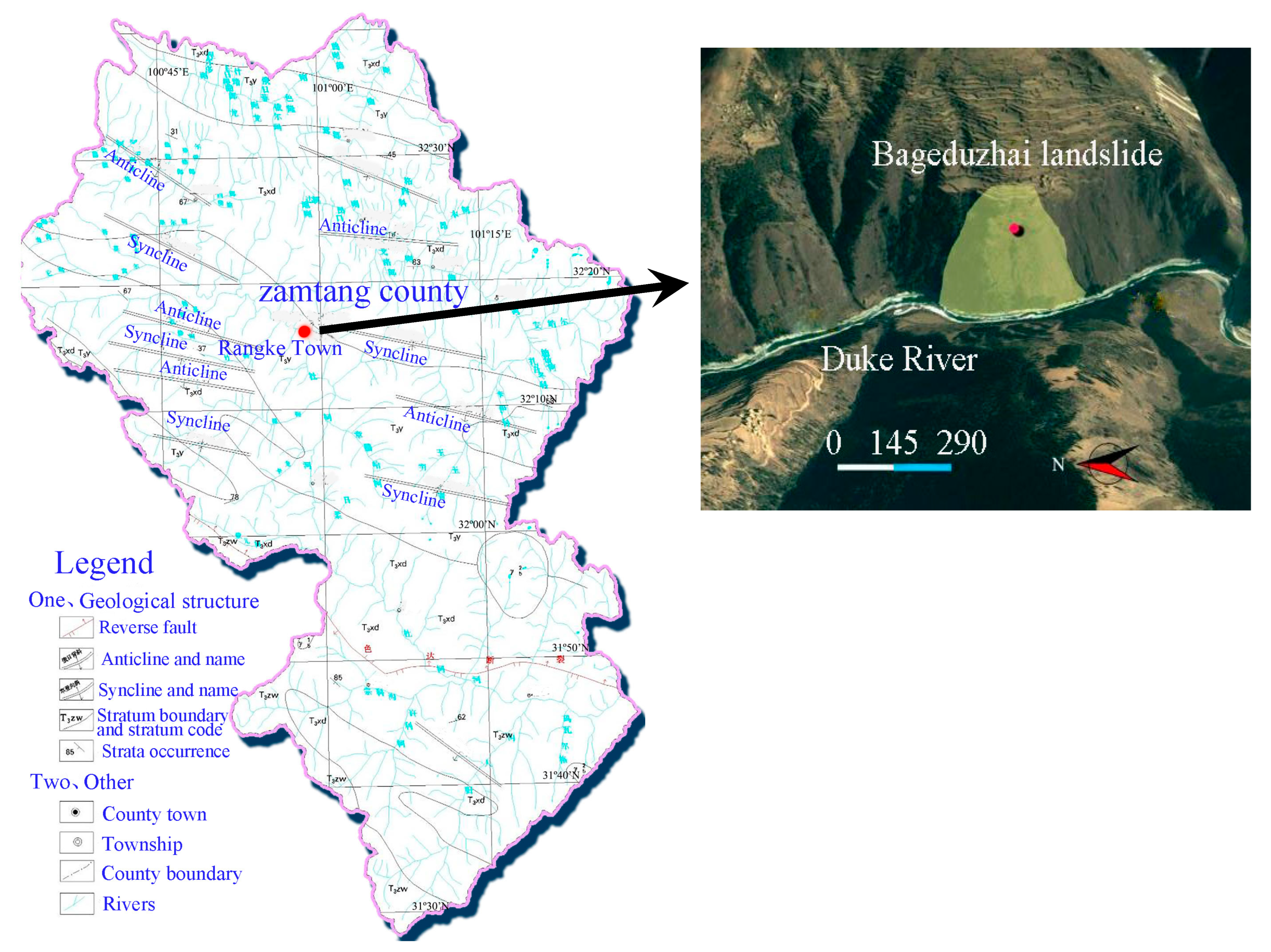
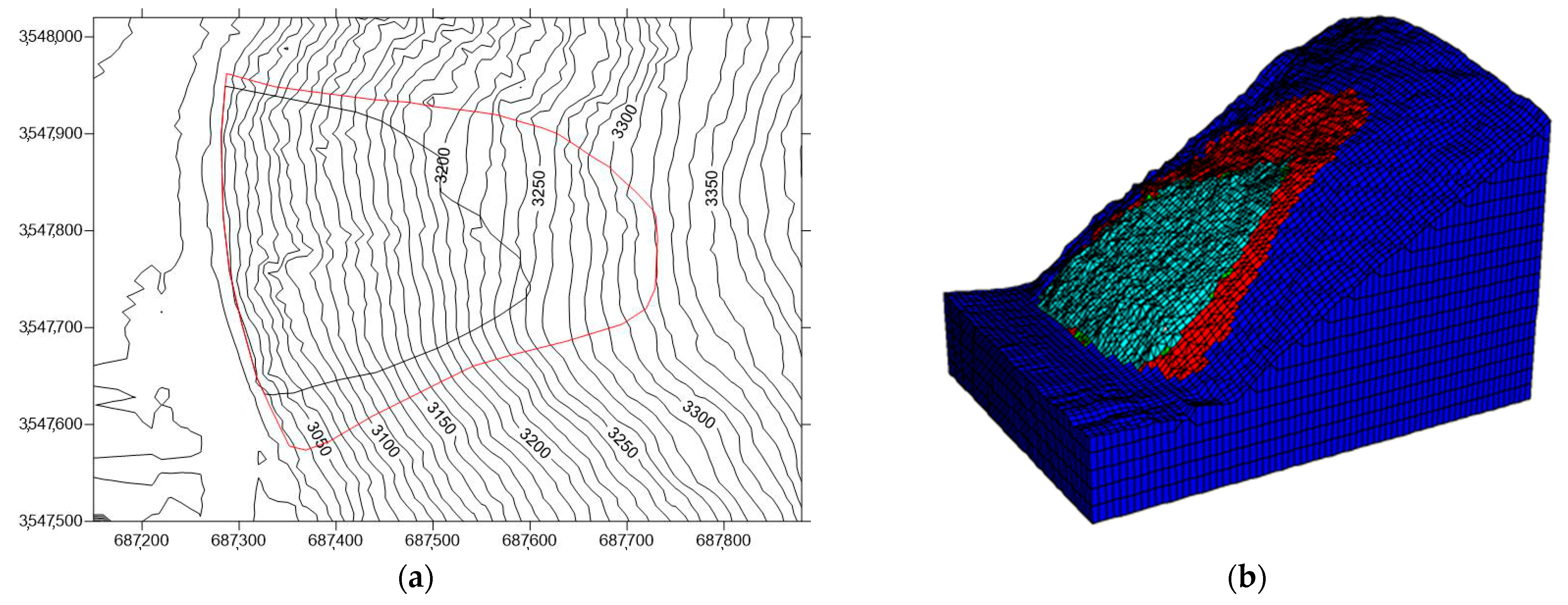
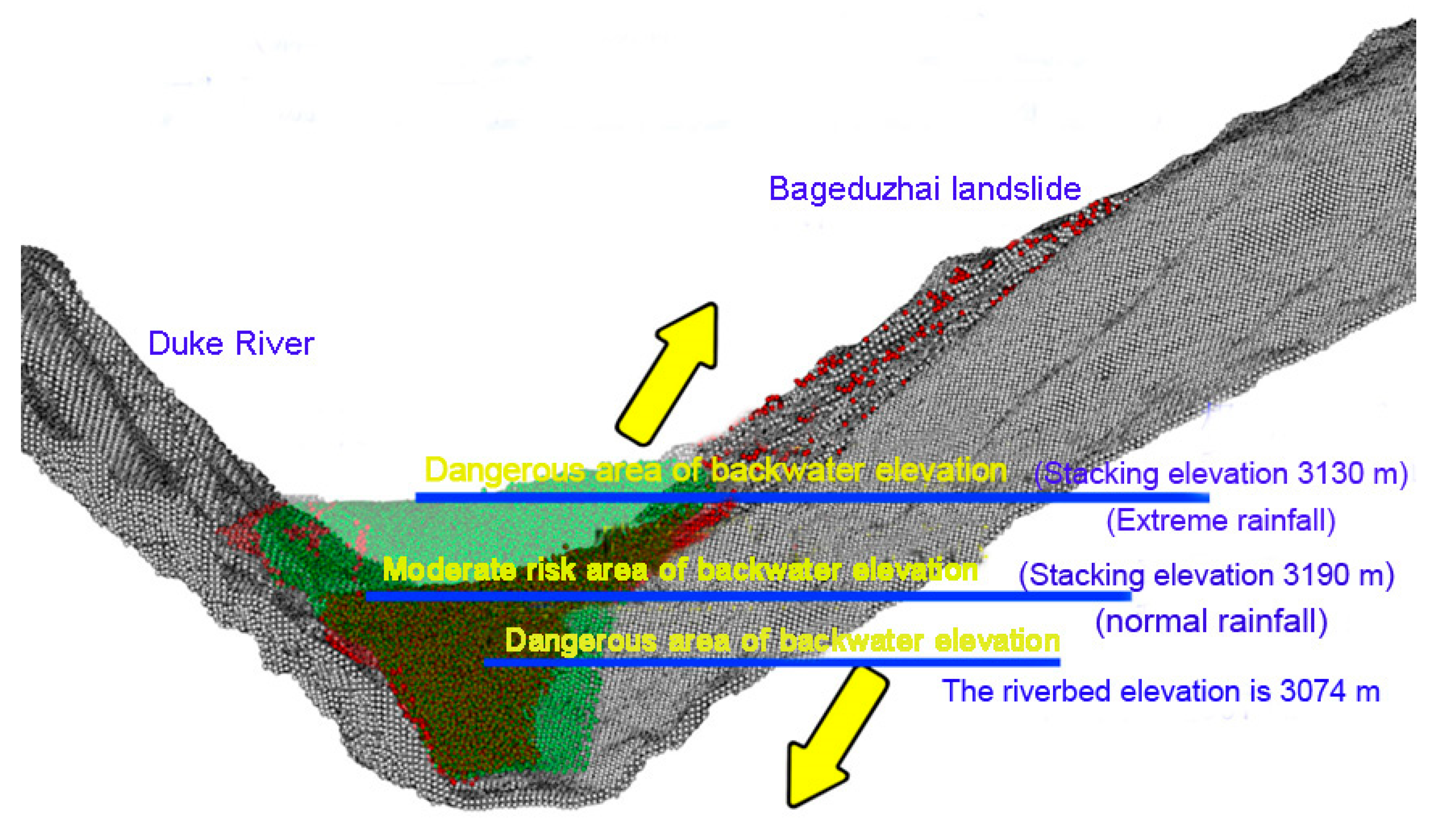
2.1. Research Area Overview

The area of the landslide is in the northern section of the Hengduan Mountains on the southeastern edge of the Qinghai-Tibet Plateau, and it belongs to the alpine plateau area of western Sichuan. It is mainly composed of tectonic erosion-caused alpine canyon landforms formed by flowing water, cold-weathering processes and ice and snow. The degree of slope-cutting is strong, the mountain is high and the valley is deep. The valley is a mostly narrow, ‘V’-shaped valley, the bank slope angle is above 40°, the valley altitude is 2650–3700 m and the relative height difference is generally greater than 1000–1500 m. The area is in the Duke River Basin in the upper reaches of the Dadu River, and the neotectonic movement is strong. The western part of the basin is composed of a series of strongly compressed linear folds and high-dip thrust faults, and the tectonic line is NW-trending. The eastern part is composed of a series of strongly compressed tight folds, and faults are not developed. From north to south, the tightness of the folds increases. The point of the Bageduzhai landslide is located at the southern end of the Rangtang syncline and the northwestern end of the Caodeng syncline. The geological sketch is shown in Figure 2.

Wuyi Village, Wuyi Township, Rangtang County, where the Bageduzhai landslide is located, is in the southern portion of Rangtang County. The landform type in the area belongs to the structurally eroded alpine landform, and the lithology combination is more complex. The exposed strata mainly include the Cenozoic Quaternary Holocene ice-water accumulation layer (Q₄^fgl), the colluvial layer (Q₄^col+dl), the aeolian loess layer (Q₄^eol), the alluvial layer (Q₄^pal) and the Triassic Upper Yajiang Formation (T₃y). The area is mainly covered in loose rock, pore water and bedrock-fissure water. Pore phreatic water mainly occurs in the sand and gravel layers of the riverbed and the terrace of the Duke River and the loose soil deposits in the gully in the middle and lower parts of the Wuyicun slope, and it is partially distributed in the Quaternary loose deposits in the slope area on both sides of the gully. Bedrock-fissure water is widely distributed in the shallow-surface weathering-unloading zones and the tectonic-fissure zones. Through the data obtained from simple hydrological observation of the borehole cuttings in the study area and the hydrogeological investigation and analysis of the landslide area, there is no groundwater level present in the borehole, the buried depth of the stable groundwater level is low and there is no stable spring point exposed in the front shear outlet area. This results in landslide deformation and the failure being less affected by the groundwater level. The Bageduzhai landslide is located in the region of the Duke River. The shear crack of the landslide is located on the inside of the road, away from the river. Our research of the stability analysis mainly focuses on obtaining the slide mass volume and the location of slide plane to provide the initial condition for dynamic process simulation. Therefore, the water level of the landslide may play a smaller role in the progress of the landslide and can be ignored.

2.2. Landslide Characteristics

2.2.1. Overall Characteristics of Landslides

The Bageduzhai landslide is a soil landslide covered by colluvial deposits and glacial water debris accumulation on the bedrock. The slope is longitudinally stepped, generally gentle and steep, with a relative height difference of approximately 300 m and a slope of approximately 40°. The rear edge is approximately 3370 m above sea level, and part of it is relatively gentle, which is a weak deformation zone. The front edge is steep, which is a strong deformation zone. The range of the strong and weak deformation zones of the landslide is shown in Figure 3.

The boundary of the trailing edge of the landslide is bounded by cracks on the gentle slope platform of the trailing edge of the landslide. The cracks are arc-shaped and are mainly from tensile deformation. The upper part of the left boundary of the landslide starts from the arc crack of the trailing edge, the middle and lower parts are bounded by the left gully and there are signs of creep on the upper left side; the upper part of the right boundary of the landslide starts at the steep and gentle junction of the slope and farmland on the right side of the landslide. There are signs of tensile deformation in the upper part of the right boundary and obvious shear cracks in the lower part of the right boundary. The boundary of the front edge of the landslide is bounded by the shear outlet at the lower part of the scarp. The shear outlet is distributed on the highway and the inner scarp of the highway, and the shear deformation is obvious. In the longitudinal direction, the thickness of the sliding body in front of the landslide is larger, and the maximum thickness of the sliding body on the west side of the landslide front reaches 32 m, while the trailing edge is thinner, only more than ten meters. Horizontally, the front part of the landslide is thicker, and the left and right sides are thinner.

The Bageduzhai landslide is a traction-falling landslide. The inner layer of the accumulation body slides, and there are multilevel accumulations. The lithology has the characteristics of a gravel soil layer-silt soil layer interbedded with a gravel layer. The sliding surface is mainly the weak surface of the silty sand of the landslide, and the sliding bed is the Quaternary colluvial gravel soil (middle and rear) and the Quaternary ice-water accumulation layer (middle and front). The sliding body is mainly composed of four layers: the Quaternary aeolian loess layer (Q₄^eol), the humus layer, the Quaternary colluvial gravel soil (Q₄^col+dl) and the Quaternary ice-water accumulation gravel layer (Q_1-3^fgl) in front of the landslide, as shown in Figure 4.

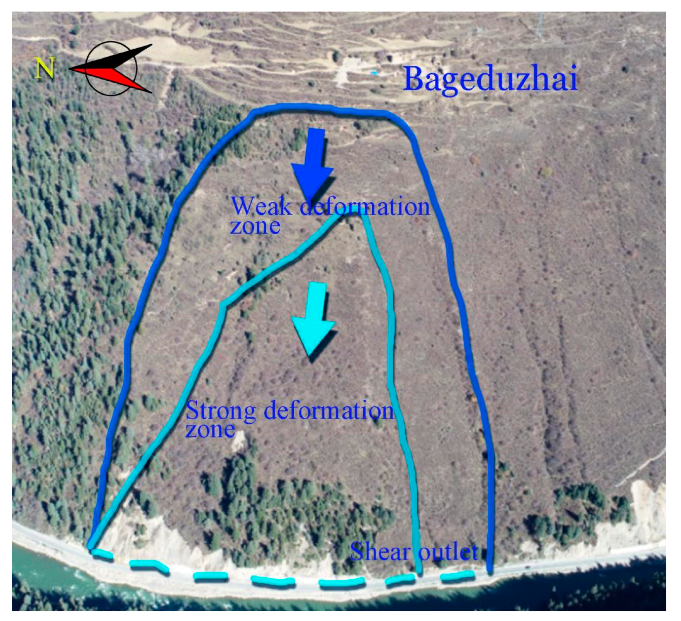
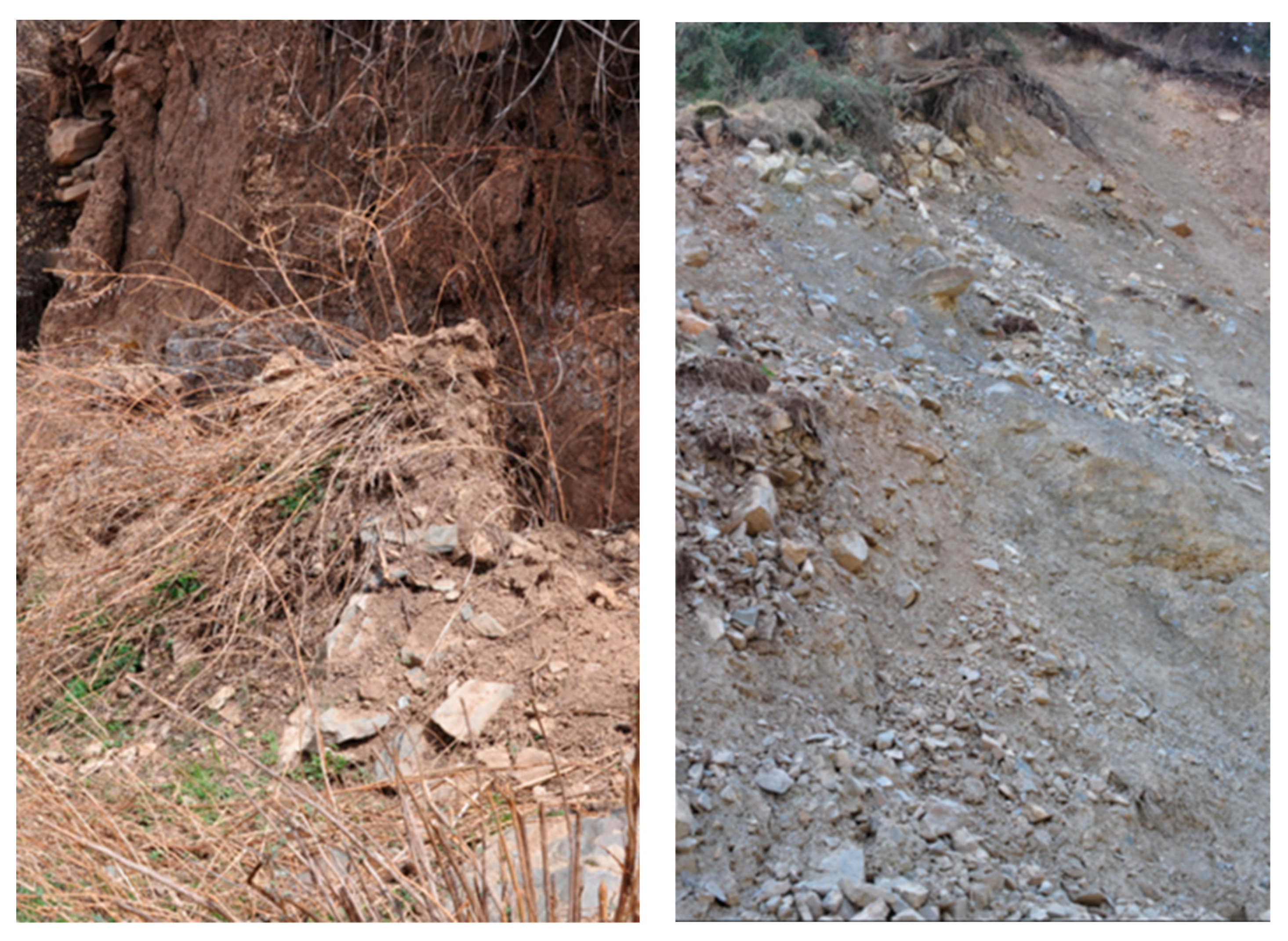
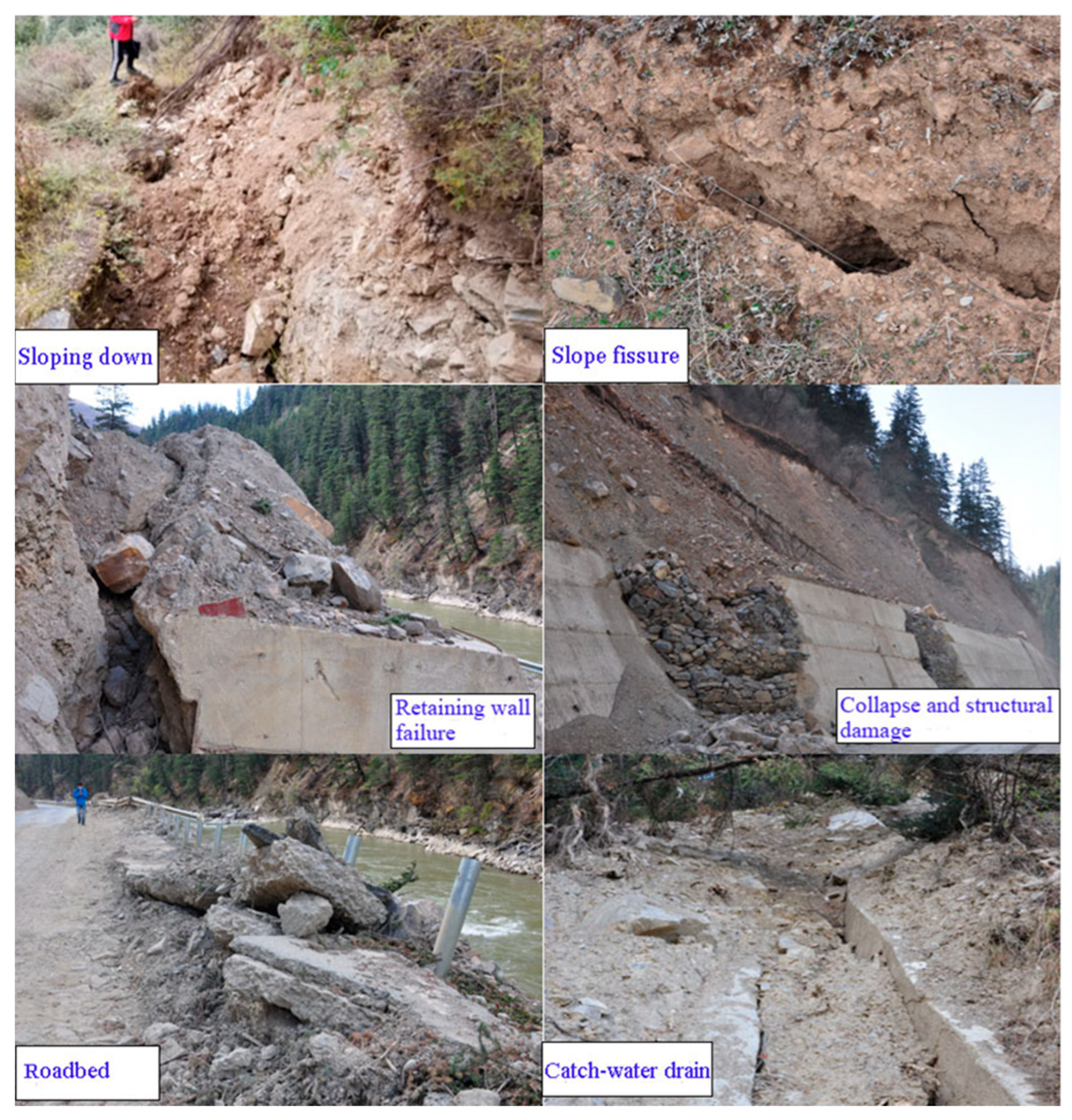
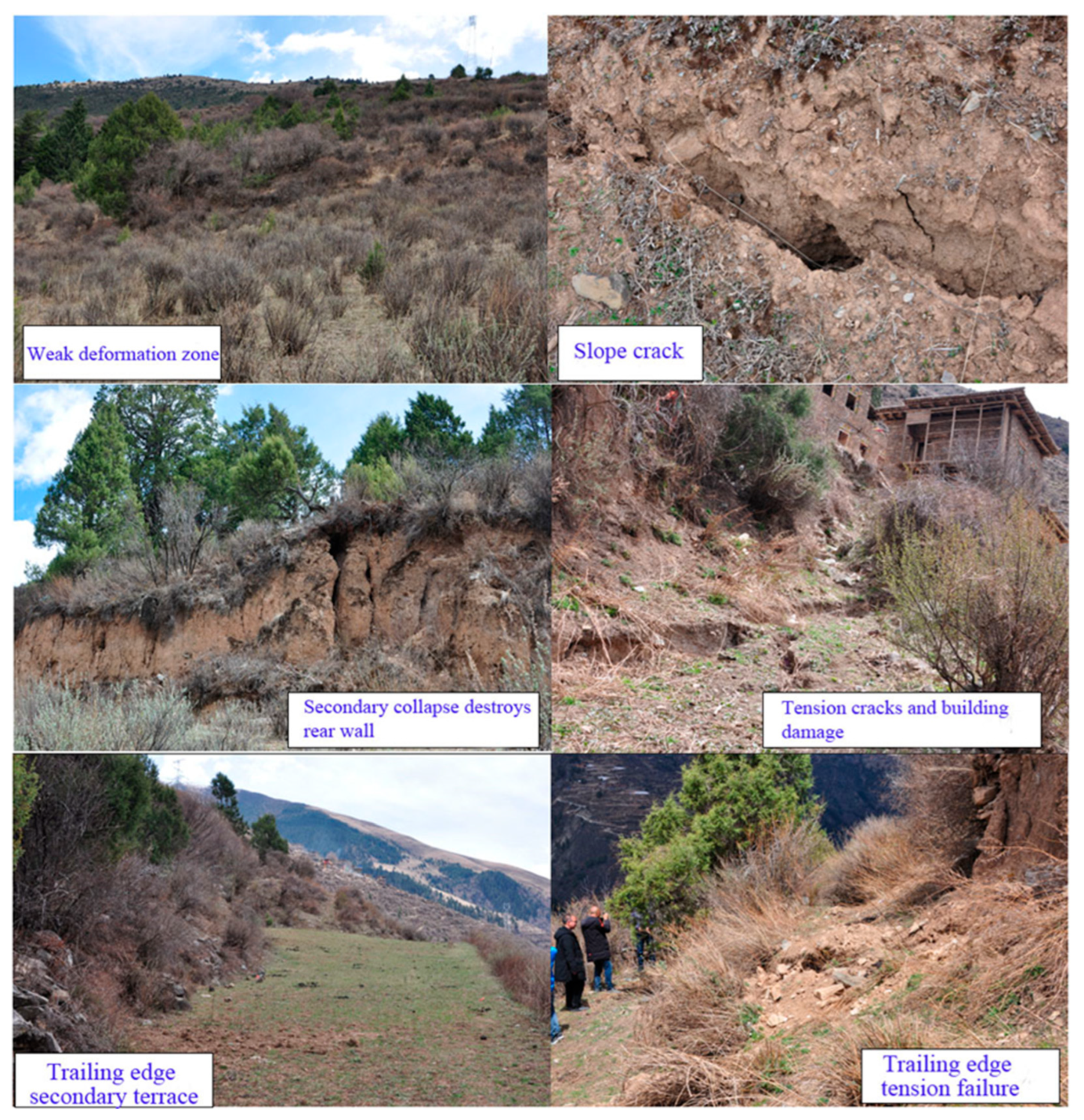
2.2.2. Landslide Deformation and Failure Characteristics

The strong deformation zone is in the middle and lower parts of the disaster body. The shape in plane view is semi-elliptical, and the elevation is stepped. The distribution elevation of the slope is 3080 m–3175 m, the width is approximately 210 m and the longitudinal length is approximately 260 m. The slope of the landslide is gentle and steep, showing a step-cliff shape. The gently sloped area is 15°–25°, and the slope of the lower free surface is nearly vertical, with an average slope of 41°. The strata in this area are mainly a Quaternary colluvial layer (Q₄^col+dl) and a Quaternary ice-water accumulation layer (Q^fgl). The boundary of the strong deformation area is a circular crack, the back wall is bright, and the crack is filled with gravel soil and plant roots. There are also seven secondary cracks in the strong deformation zone, with multiple levels of scraping, obvious local dislocation cracking, loose and broken rock and soil mass, which are easily aggravated by rainfall or earthquakes. The shear outlet of the front edge of the strong deformation zone is the G227 National Highway and the Duke River. The high and steep excavation slope inside the highway has collapsed under the action of valley incision and air unloading, which is manifested by the outward deformation of the highway retaining wall, the bulging deformation of the steel gabion, the bulging soil crack and the local collapse deformation, as shown in Figure 5.

The weak deformation zone is located at the trailing edge of the landslide and on both sides of the strong deformation zone. The shape in plane view is of crescent-shape, the side is stepped and the shape of the whole is ‘ladder-cliff-like’. The slope of the gently-sloped area is 10°–20°, and the slope of the lower free surface is nearly vertical, with an average slope of 68°. Affected by rainfall, earthquakes, topography, zones of strong deformation and other factors, the slope for a long time has been in the creep deformation stage. It is mainly manifested as tensile cracks at the trailing edge, with slight shear cracking present next to the strong deformation zone, and local collapse at the leading edge. A total of seven cracks developed in the weak deformation zone, which mainly developed on the trailing edge and both sides, showing the characteristics of tensile failure. The deformation characteristics of the weak deformation zone on the left side of the landslide are generally not as obvious and mainly manifested as sporadic local collapse, as shown in Figure 6.

2.2.3. Instability Mechanism of the Bageduzhai Landslide

Through analysis of the above data, the Bageduzhai landslide is a slide in the inner layer of the accumulation body. The accumulation body is the Quaternary (middle and rear) collapsing gravel soil, and the middle and front part is the Quaternary ice-water accumulation layer. The mechanical properties of the weak silty-sand surface between the multiple-layer accumulations deteriorate rapidly under the action of rainfall, forming a multi-level traction landslide. This is due to the long-term unloading and seismic action of the landslide body, and the unloading fissure or seismic fissure is first formed in the free section of the original slope. Under the action of rainfall, rainfall infiltration reduces the c and φ values of the sliding body and increases the self-gravity of the sliding body. The original stress conditions of the slope are changed by river scouring at the foot of the slope and the influence of human engineering activities, which leads to the first slip in the middle and front of the slope. After losing the front support in the middle and rear of the landslide, the sliding mode of traction-falling appears as a whole. At this stage, most of the slope toe of the front edge of the landslide has been destroyed and has slipped, resulting in the loss of support in the middle and front slopes, and the rear part of the landslide is a weak deformation zone and is in a creeping state.

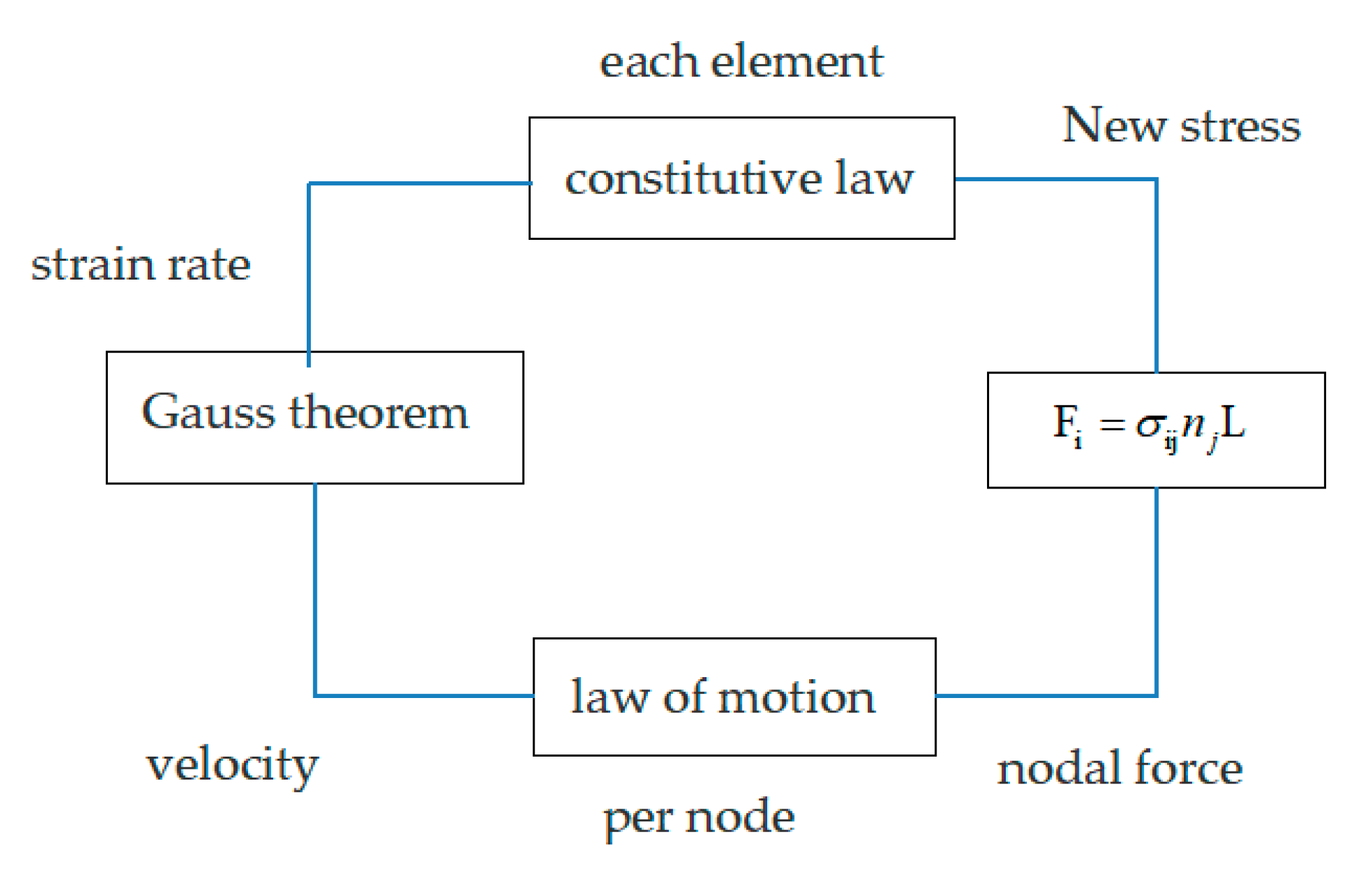
3. Calculation Conditions and Parameter Calibration

3.1. Calculation Conditions

Because the landslide is close to the Duke River and the 227 National highway, its instability and collapse can not only directly cause an impact on the national highway by burying the roadway but also pose risk by the blocking the river, which poses a serious threat to both the upstream and downstream river flow. Therefore, it is necessary to analyze the stability and river-blocking risk of the Bageduzhai landslide based on the survey results. According to our investigation, the landslide can be divided into two parts. The first part is the strong deformation zone of the upper layer, and the second part is the weak deformation zone of the lower layer. Therefore, in our simulation, two rainfall conditions are set to divide the sliding state caused by rainfall in the upper layer and the sliding state caused by rainfall in both layers. According to the investigation results, the stability of the weak deformation layer can be calculated after removing the strong deformation layer. To quantitatively study the stability, the instability mode of failure and the movement accumulation law of the Bageduzhai landslide, two types of conditions for calculation are set up on the basis of considering the geological environment characteristics of the landslide area:

Rainfall conditions: This condition considers the case of abundant rainfall, and the in-field drainage system cannot effectively drain. At this time, the hydrostatic pressure in the landslide rises rapidly, the effective stress of the soil decreases, the shear capacity decreases and the effective friction inside the landslide weakens. This condition considers the instability of the strong deformation zone of the leading edge when the front of the landslide is close to being saturated; the strength reduction factor is set to 0.9.

Extremely high-intensity rainfall conditions: This condition considers the failure of the drainage system in the field, the saturation of the landslide body and the overall sliding instability of the slope under extremely high-intensity and continuous long-term rainfall events; the strength reduction factor is set to 0.8.

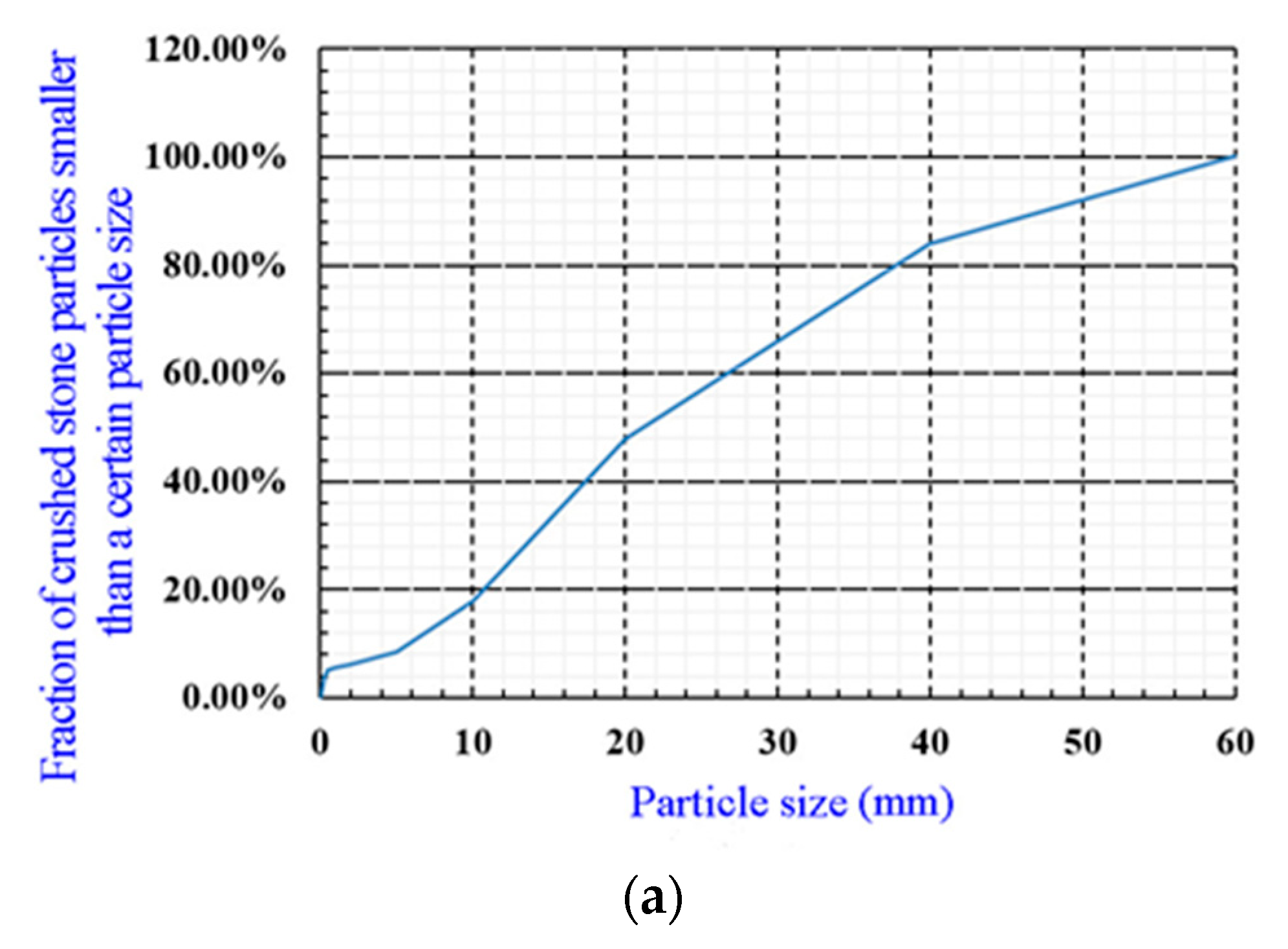
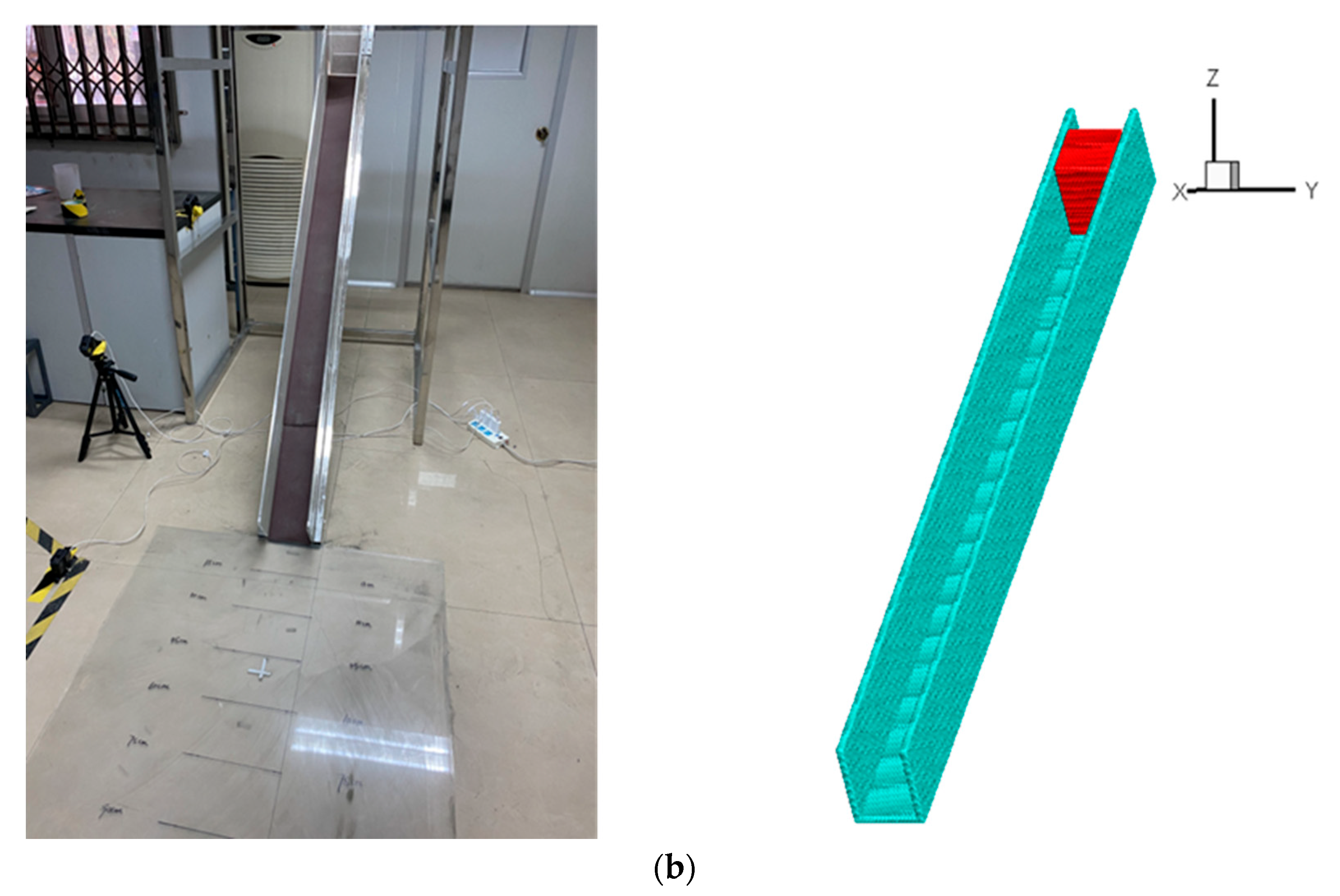
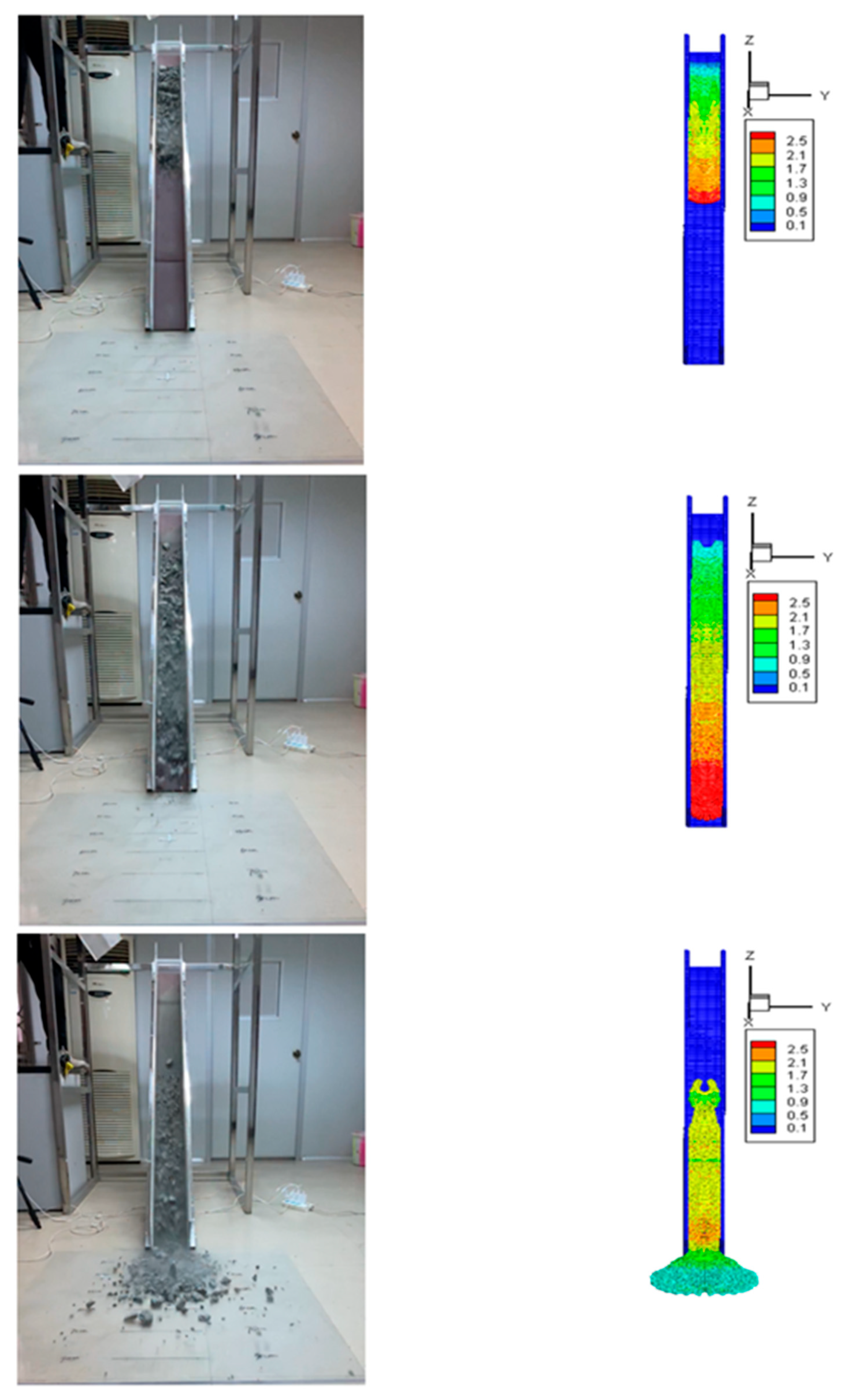
3.2. Calculation Parameters

To obtain the landslide calculation parameters and the conventional physical and mechanical parameters required for numerical calculation, the landslide body and soil samples in the sliding zone were collected to carry out indoor testing. Draw the particle size distribution curve of the landslide used in the experiment through screening experiments. The results of the screening experiment are shown in the grading curve in Figure 7a. The flume experiment was built indoors to simulate the landslide movement, and the process of landslide movement was recorded by motion-capture camera equipment. Then, a 1:1 numerical flume model was constructed to restore the movement process of the landslide materials to calibrate the calculation parameters. The physical and numerical models of the flume test are shown in Figure 7b.

The material of the flume model was a smooth high-strength acrylic plate with a total length of 2200 mm, a width of 150 mm, two arms that were 200 mm high and an inclination angle of 40°. Sandpaper was laid on the bottom of the flume. Three GoPro cameras were set up at the top, bottom and side of accumulation, and the high-speed video-recording capability of the iPhone 11 Pro Max was used to capture and record the motion form on the front of the model. According to the physical flume model size, a 1:1 reduced SPH flume numerical model was constructed. A total of 27,040 landslide particles and 100,320 flume particles were created. The numerical simulation used the Drucker–Prager criterion to describe the instability process of the landslide body. The Bingham model was used to describe its movement process, and the dilatancy behavior during the movement of the landslide body was ignored. In comparison with the boundary conditions of contact solid boundary condition [33], the dynamic solid boundary can mitigate boundary particle defects, and in comparison with the symmetric virtual particle boundary condition, the dynamic solid boundary has an advantage in building complex boundary [34]. The flume was described by the dynamic boundary conditions. The specific numerical implementation process can be found in the following research papers [25,26,27,28].

The SPH numerical simulation results are compared with the results of the actual indoor flume physical model experiment. The flow material is treated as dry granular in simulation to be consistent with the experiment. As shown in Figure 8, the results of the flume physical model and the SPH numerical simulation at 500 ms, 900 ms and 1400 ms are selected. In the simulation, different friction angles of landslide material and friction coefficient of solid boundary are evaluated to simulate the channel experiments until the simulation results agree well with the experimental results. The results show that when the internal friction angle of the landslide material is set to be 30°, the friction coefficient between the sandpaper and the landslide is 0.4 and the friction coefficient between the landslide and the acrylic plate is 0.3; the calculated simulation results are better reproduced and agree well with the experiment results.

The calculation parameters under natural conditions are shown in

Table 1. Geotechnical mechanical parameters.

Rock	Bulk Modulus K (GPa)	Shear Modulus G (GPa)
Bed rock	2.00	1.600
Secondary slip zone	0.07	0.062
Main sliding belt	0.07	0.062
Landslide mass	0.08	0.075

and

Table 2. Geotechnical mechanical parameters.

Rock	Density (kg/m3)	Cohesion (MPa)	Friction Angle (°)
Bed rock	2500	1.2	35
Secondary slip zone	2200	0.1	22
Main sliding belt	2250	0.15	25
Landslide mass	2300	0.18	28

. Because it is difficult to obtain complete samples from the landslide, the elastic parameters were provided by the investigation by the partner testing company and adjusted according to empirical in Table 1. The friction coefficient was obtained from the experiment of dry granular flow in channel and adjusted according to empirical in Table 2. The rainfall conditions did not consider the case of abundant rainfall, and the interception and drainage system in the field cannot drain effectively. Considering that the rock and soil is 80% saturated, the working condition parameters are 0.9-times the parameters under natural conditions. The extremely high-intensity rainfall conditions are extremely common, and rainfall events occur frequently in the long-term; the landslide body is completely saturated, and the overall sliding instability of the slope of the body is taken as 0.8-times the natural condition.

4. Landslide Deformation and Stability Analysis under Different Conditions

The FLAC method is used to obtain the stress and deformation values of each element (or node) on the slope at each time step by iterative solution, and the whole slope deformation and failure process is simulated. The Lagrangian difference method calculation cycle is shown in Figure 9.

To obtain high-precision data of the terrain of the field area, a UAV is used to image the field area, and then a high-precision topographic map is constructed, as shown in Figure 10a. The landslide stability calculation model is constructed according to the topographic map, as shown in Figure 10b. The deformation and failure mode of the slope under the action of gravity is analyzed. Horizontal tectonic stress is not applied in the model, and the side-edge boundary and the bottom boundary of the model are in the form of a one-way constraint.

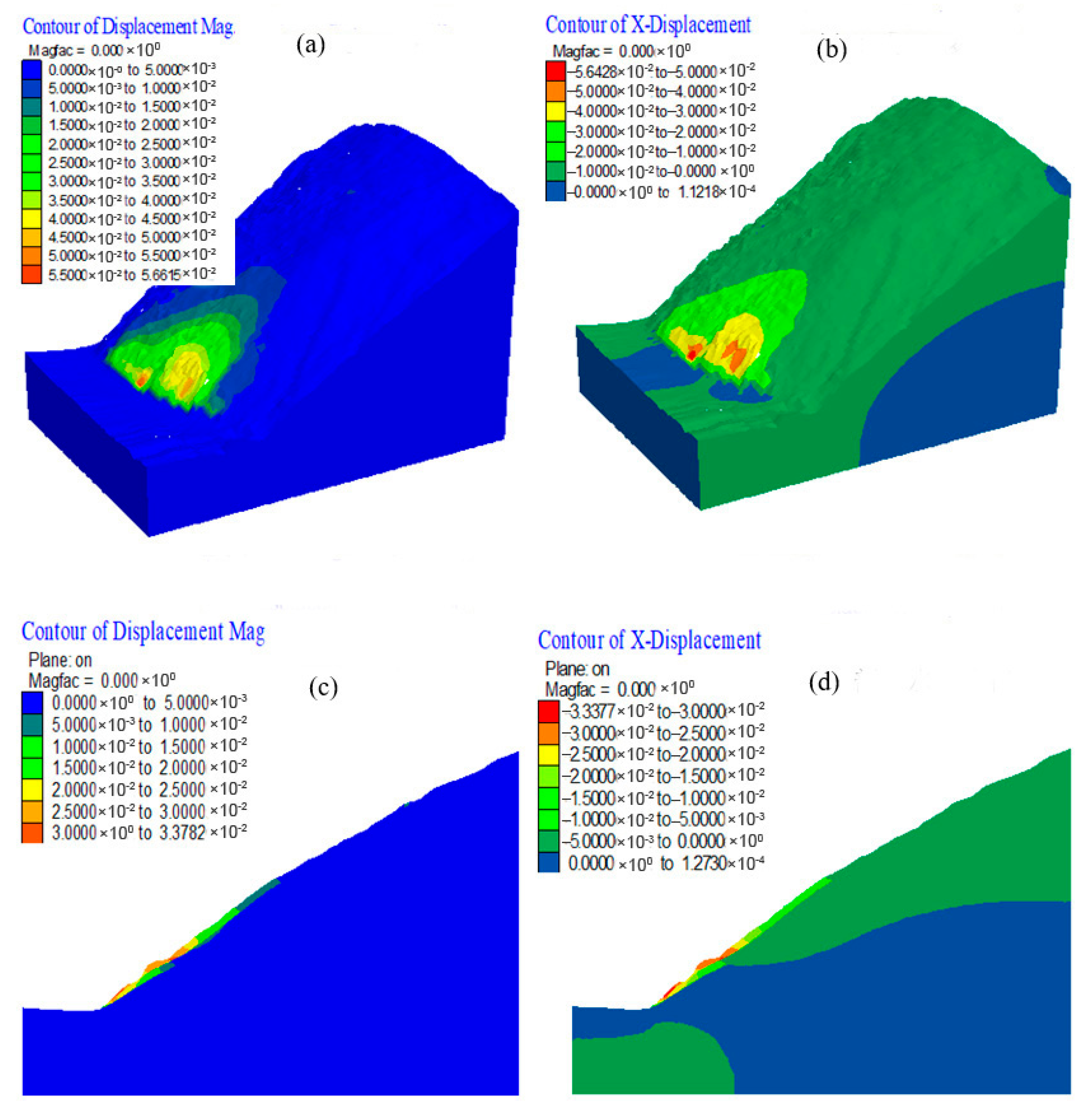
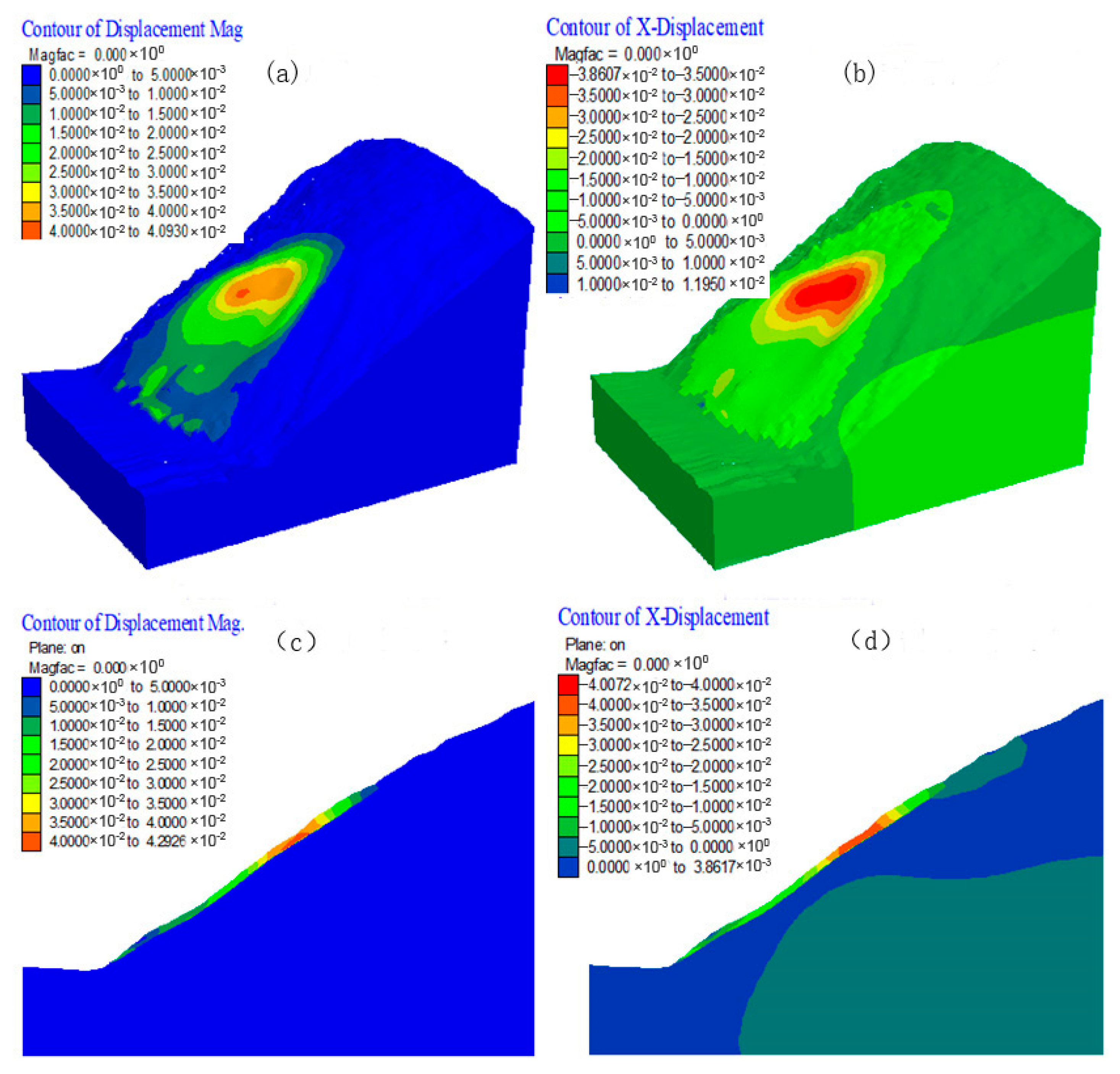
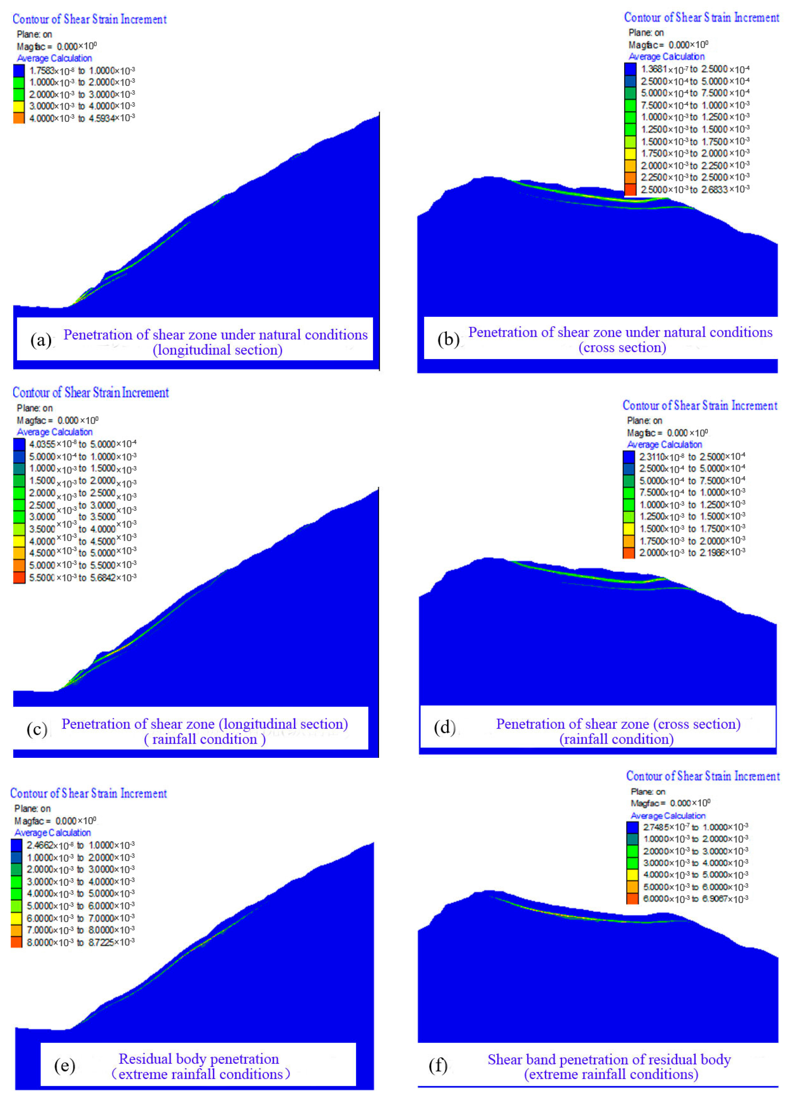
4.1. Deformation Characteristics of Landslides under Ordinary Rainfall Conditions

The stress state of the landslide after strength reduction is analyzed, and the stress field characteristics are shown in Figure 11.

According to the stress field distribution map, under ordinary rainfall conditions, except for a certain depth range from the surface, the landslide is affected by the lithology, rock mass structure and valley-slope morphology that produce different degrees of stress concentration and differentiation. The stress field is dominated by self-weight stress. Due to the inhomogeneity of the slope structure, especially the existence of weathered rock masses in the slope, the distribution of the minimum principal stress has obvious inhomogeneity or zoning.

To analyze the deformation and failure characteristics of the landslide, the displacement is analyzed, and the displacement cloud diagram is shown in Figure 12.

Figure 12 shows that the displacement change of the landslide is mainly concentrated in the middle and lower parts and is mainly a horizontal deformation. The maximum displacement of the landslide is approximately 6 cm, and the expansion of the deformation concentration area of the landslide is obvious. It can be inferred that the landslide can be destabilized and destroyed under ordinary rainfall conditions, and the slope in the strong deformation zone can slide.

4.2. Deformation Characteristics of Landslides under Extremely High-Intensity Rainfall Conditions

Considering the strong deformation zone is unstable under ordinary rainfall conditions, it is only necessary to analyze the stress distribution state and displacement variation characteristics of the weak deformation zone after the instability of the strong deformation zone. The stress field cloud diagram is shown in Figure 13.

It can be seen by comparing Figure 11 and Figure 13 that there is a certain difference between the maximum principal stress field after the sliding of the front strong deformation sliding body and the stress field distribution when it does not slide. However, the stress field within a certain range of the slope after excavation is still dominated by gravity. The magnitude of the maximum principal stress gradually increases with increasing depth from the slope surface. After the sliding of the front sliding body, a certain degree of stress concentration area appears in the residual landslide body, but the area is small, and the magnitude increases little. The minimum principal stress also has a reduction zone, that is, the stress release zone, but the area is small, and the degree of stress release is also small. Therefore, it can be judged that the slope has been in a state of low safety reserve in the initial state, the slope stability has declined and it may presently be in an unstable state.

The displacement variation characteristics of the weak deformation zone under extreme rainfall conditions are simulated. The displacement cloud is shown in Figure 14.

Figure 14 shows that the deformation of the landslide in the weak deformation zone under extreme rainfall conditions is mainly concentrated in the upper part of the slope, showing a push-type failure. In general, after the front of the strong deformation sliding body slides, a continuous deformation concentration area is formed in the upper part of the landslide.

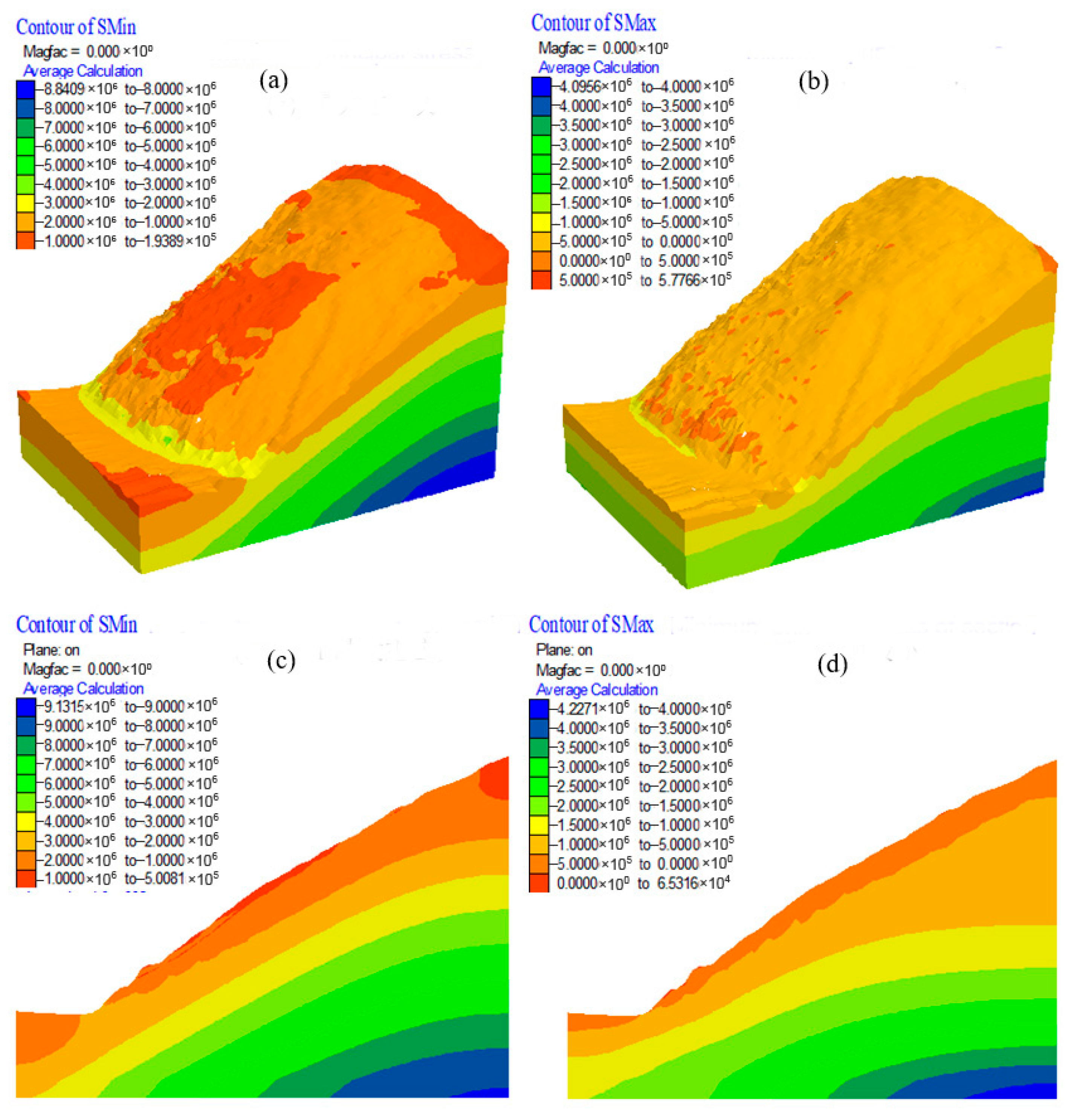
4.3. Landslide Stability Analysis

The stability of the landslide under natural conditions, ordinary rainfall conditions and extreme rainfall conditions is calculated. The potential sliding surface of the landslide under different conditions is shown in Figure 15.

Figure 15 shows that under natural conditions, the sliding surface of the strong deformation zone of the landslide is mostly connected, and the main sliding surface is small, indicating that under natural conditions, possibility of overall sliding of the landslide is small. Under the condition of rainfall, the sliding surface of the strong deformation zone of the leading edge is basically completely penetrated, and the main sliding surface is less penetrated. The landslide may be destroyed along the sliding surface of the strong deformation zone of the leading edge, and the possibility of overall sliding is not large. Under extreme rainfall conditions, the strong deformation zone at the leading edge of the landslide slides, and the weak deformation zone at the trailing edge is close to the overall penetration. Among them, the degree of penetration of the middle and upper parts of the main sliding surface is large, and the weak deformation zone at the trailing edge may be cut out from the middle of the landslide.

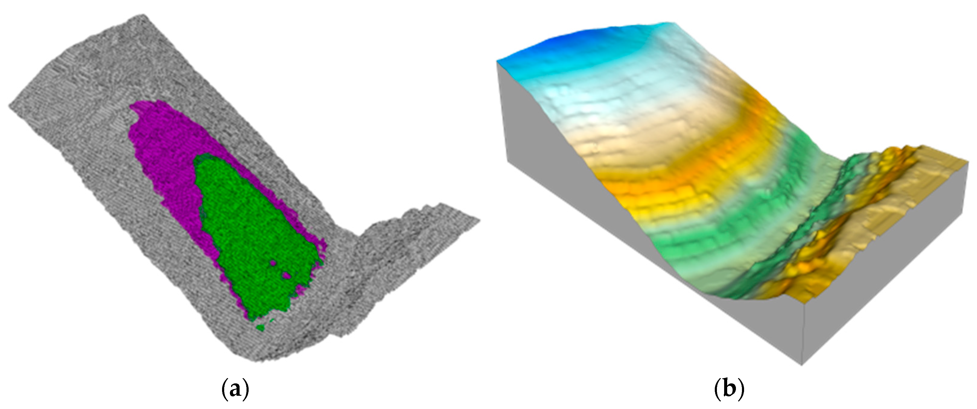
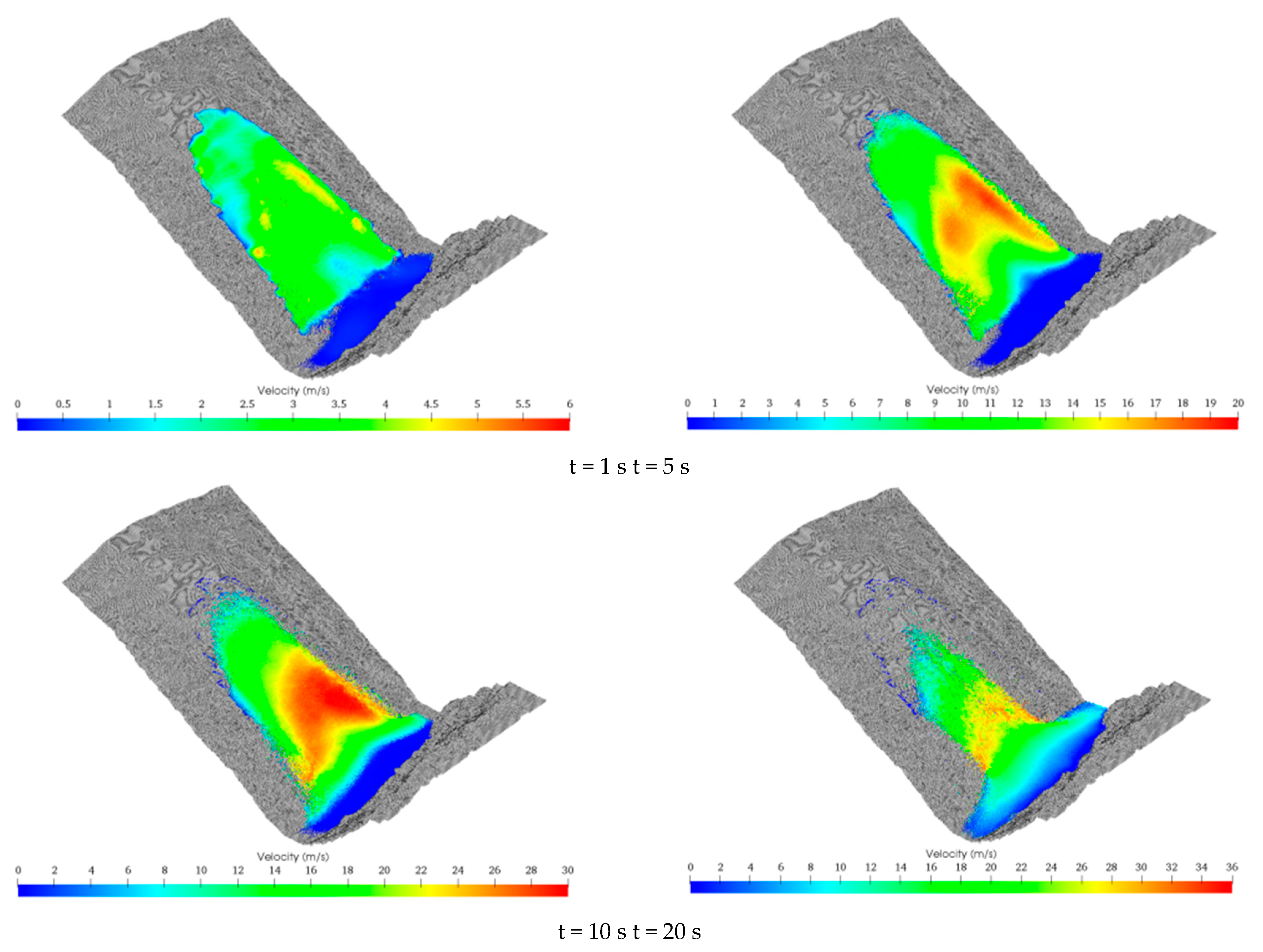
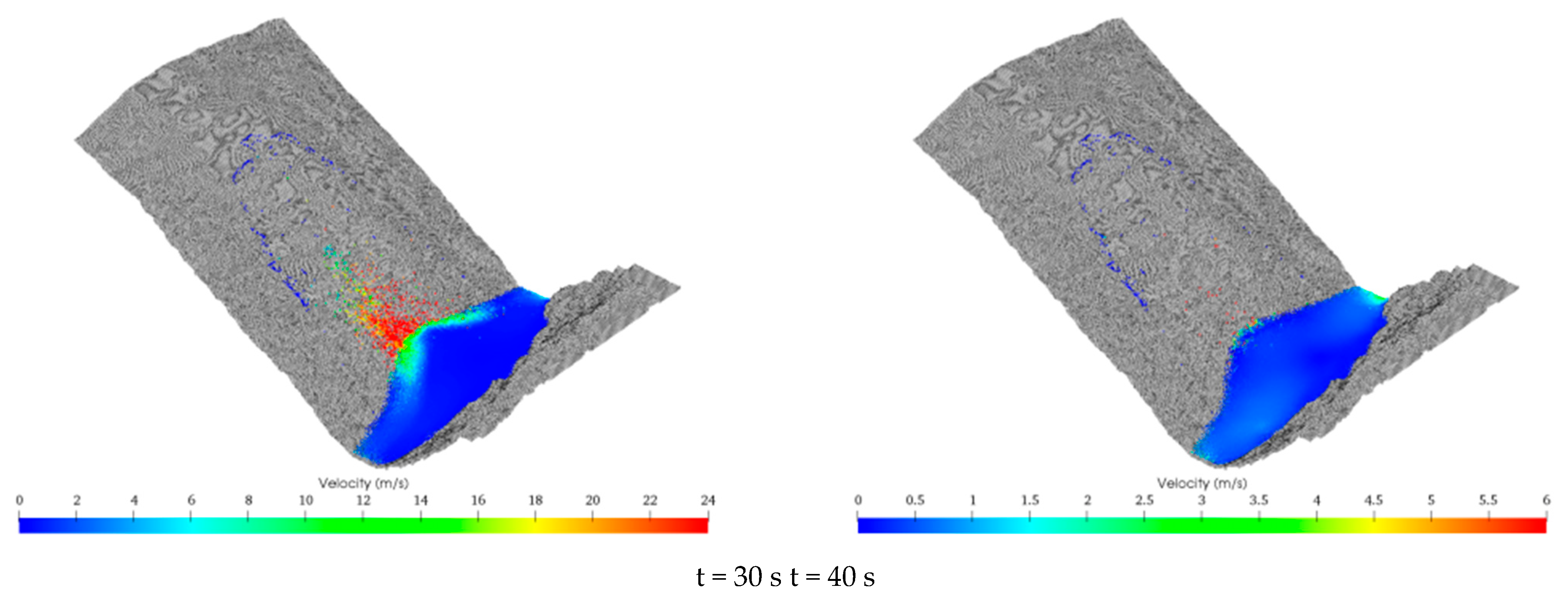
5. Landslide Dynamics Analysis under Different Conditions

The smoothed particle hydrodynamics (SPH) method solves partial differential equations or integral equations through a series of interaction points carrying material information. The construction of the SPH equation is divided into two key steps. The first step is the smooth approximation of the kernel function, and the second step is the particle approximation of the kernel function.

Based on the Lagrangian description, the basic rules of mass conservation, momentum conservation and energy conservation can be written as Navier–Stokes partial differential equations, as shown below:

$$\left\{\begin{array}{l}\frac{D\rho }{Dt}=-\rho \frac{\partial {\mathit{v}}^{\beta }}{\partial {\mathit{x}}^{\beta }}\\ \frac{D{\mathit{v}}^{\alpha }}{Dt}=\frac{1}{\rho }\frac{\partial {\mathit{\sigma }}^{\alpha \beta }}{\partial {\mathit{x}}^{\beta }}+{\mathit{F}}^{\alpha }\end{array}\right.$$

(1)

The superscript represents the coordinate direction, $\rho$ is the density, $\mathit{v}$ is the velocity, $\sigma$ is the stress tensor, $\mathit{F}$ is the volume stress component and $t$ is the time. The SPH form of the equation can be written as:

$$\frac{D{\rho }_i}{Dt}={\rho }_i{\displaystyle \sum _{j=1}^N\frac{m_j}{{\rho }_j}{\mathit{v}}_{ij}^{\beta }\frac{\partial W_{ij}}{\partial {\mathit{x}}_i^{\beta }}}$$

(2)

In addition, the momentum equation in the form of SPH method can be written as:

$$\frac{D{\mathit{v}}_i^{\alpha }}{Dt}={\displaystyle \sum _{j=1}^N{m}_j(\frac{{\sigma }_i^{\alpha \beta }}{{\rho }_i^2}+\frac{{\sigma }_j^{\alpha \beta }}{{\rho }_j^2})\frac{\partial W_{ij}}{\partial {\mathit{x}}_i^{\beta }}}+{\mathit{F}}_i{}^{\alpha }$$

(3)

In the dynamic boundary method, the solid wall boundary is represented by multiple layers of virtual particles with fixed positions; in this study, the Bingham fluid model is used to describe the dynamic evolution process of the landslide. The Bingham fluid model can be written as:

$${\mathit{\sigma }}^{\alpha \beta }=-p{\delta }^{\alpha \beta }+2(\eta +\frac{{\tau }_{\min }}{\dot{\gamma }}){\dot{\mathit{e}}}^{\alpha \beta }$$

(4)

$${\dot{\mathit{e}}}^{\alpha \beta }={\dot{\mathit{\epsilon }}}^{\alpha \beta }-\frac{1}{3}{\dot{\mathit{\epsilon }}}^{\kappa \kappa }{\delta }^{\alpha \beta }$$

(5)

In the formula, p is the pressure of rock and soil, ${\delta }^{\alpha \beta }$ is the Kronecker symbol, $\eta$ is the viscosity coefficient of large deformation of rock and soil, ${\tau }_{\min }$ is the yield stress, $\dot{\gamma }$ is the pure shear strain rate, ${\dot{\mathit{e}}}^{\alpha \beta }$ is the deviatoric strain rate tensor and ${\dot{\mathit{\epsilon }}}^{\alpha \beta }$ is the strain rate tensor, and its definition is as follows:

$${\dot{\mathit{\epsilon }}}^{\alpha \beta }=\frac{1}{2}(\frac{\partial {\mathit{v}}^{\alpha }}{\partial {\mathit{x}}^{\beta }}+\frac{\partial {\mathit{v}}^{\beta }}{\partial {\mathit{x}}^{\alpha }})$$

(6)

In the formula, ${\mathit{v}}^{\alpha }$ and ${\mathit{v}}^{\beta }$ are the fluid velocities, and ${\mathit{x}}^{\alpha }$ and ${\mathit{x}}^{\beta }$ are fluid coordinates.

The yield strength based on the Drucker–Prager yield criterion can be defined as:

$${\mathit{\tau }}_{\min }=-\mu p+c$$

(7)

In the formula, $\mu$ is the friction coefficient of rock and soil, and c is the cohesion.

According to the static analysis results, the sliding surface information is obtained, and then the dynamic numerical calculation model is constructed, as shown in Figure 16a, which contains 203,412 boundary particles and 107,079 slope particles. The distance between particles in the X-, Y- and Z-directions is 10 m (Figure 16b). The dynamic processes of the Bageduzhai landslide under different rainfall conditions is analyzed. The calculation conditions are divided into ordinary rainfall conditions and high-intensity rainfall conditions. The sliding accumulation of the instability and the failure in front of the landslide is calculated under ordinary rainfall conditions. Under high-intensity rainfall conditions, two sliding accumulations in the deformation zone before and after the high-intensity rainfall are calculated.

In this model, the landslide is broken and disintegrated during the sliding process, which is regarded as a Bingham fluid after failure occurs, and in the simulation, cohesion is ignored. The internal friction coefficient is reduced in the landslide motion simulation, and the parameters in

Table 3. Dynamic simulation parameters of the Bageduzhai landslide.

Compressive Parameters of State Equation of Landslide Mass	B (GPa)	4.00 × 107
Internal friction coefficient under normal rainfall conditions	${\mu }_1$	0.404 (22°)
Internal friction coefficient under high-intensity rainfall condition	${\mu }_2$	0.363 (20°)
Viscosity coefficient	η (Pa·s)	0.01

are used for calculation.

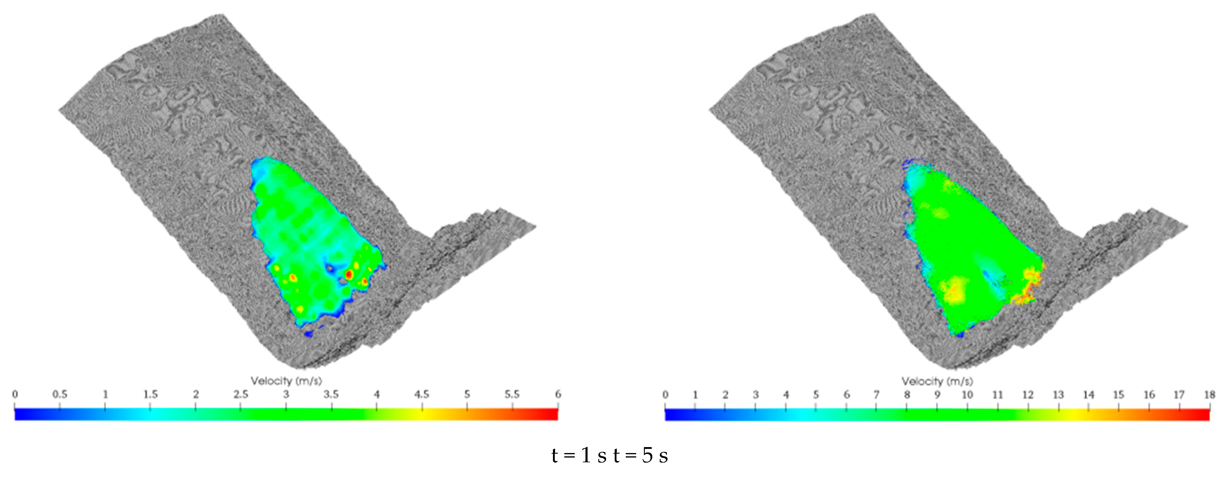
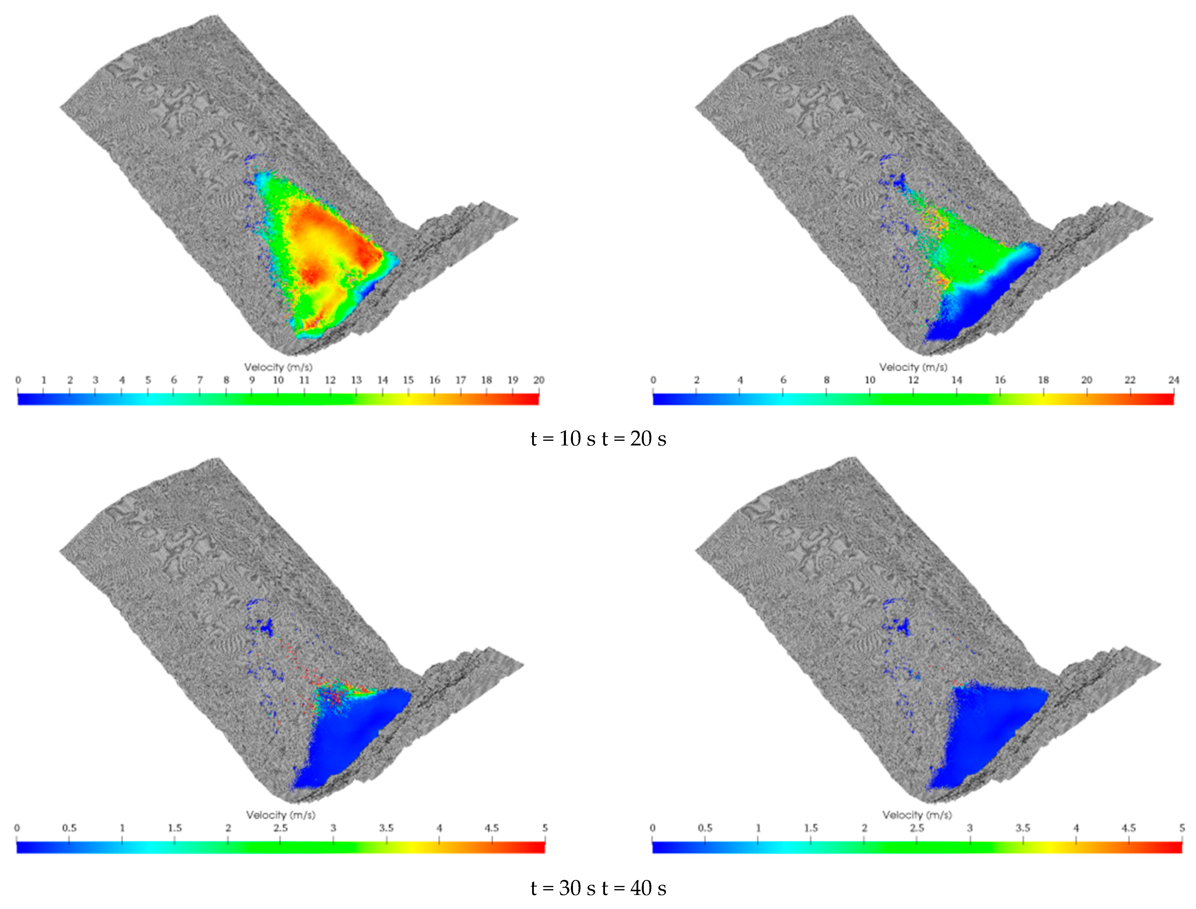
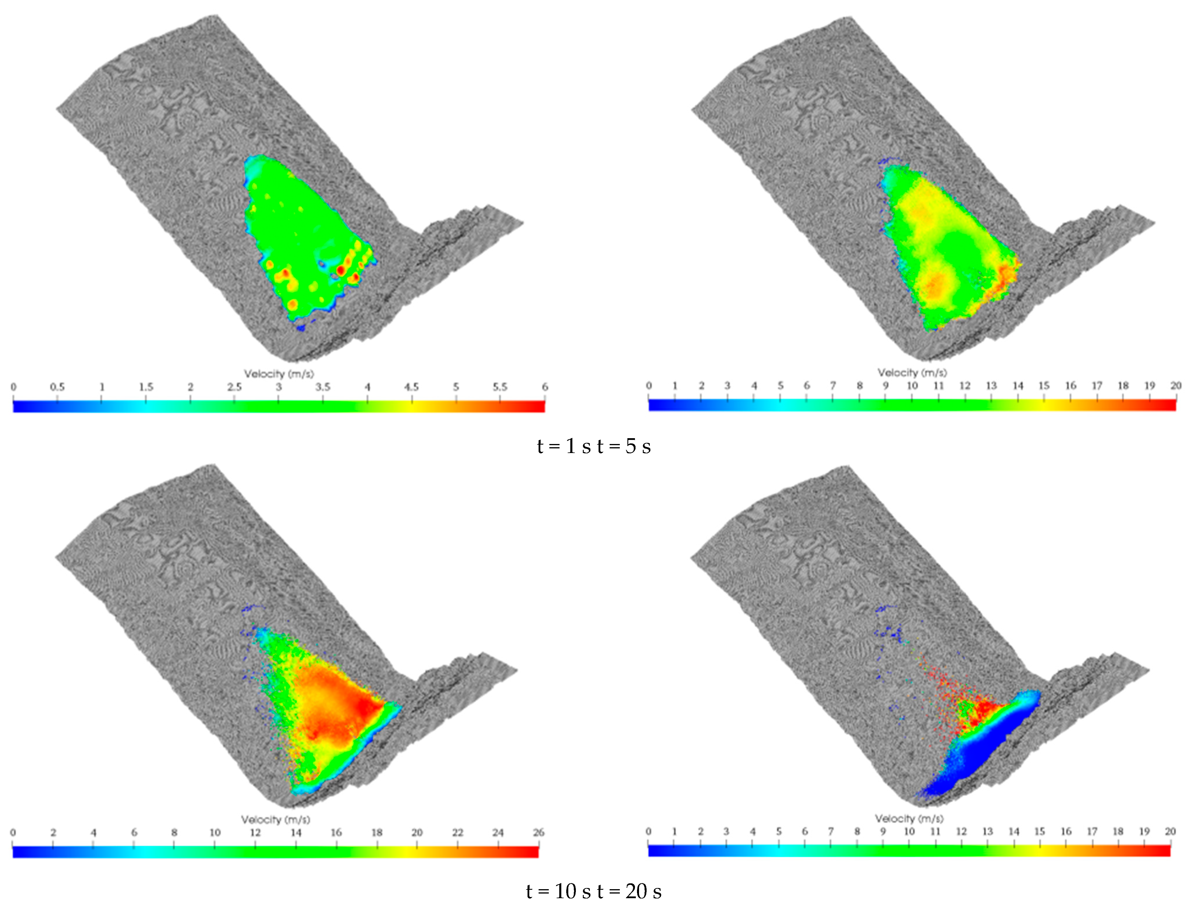
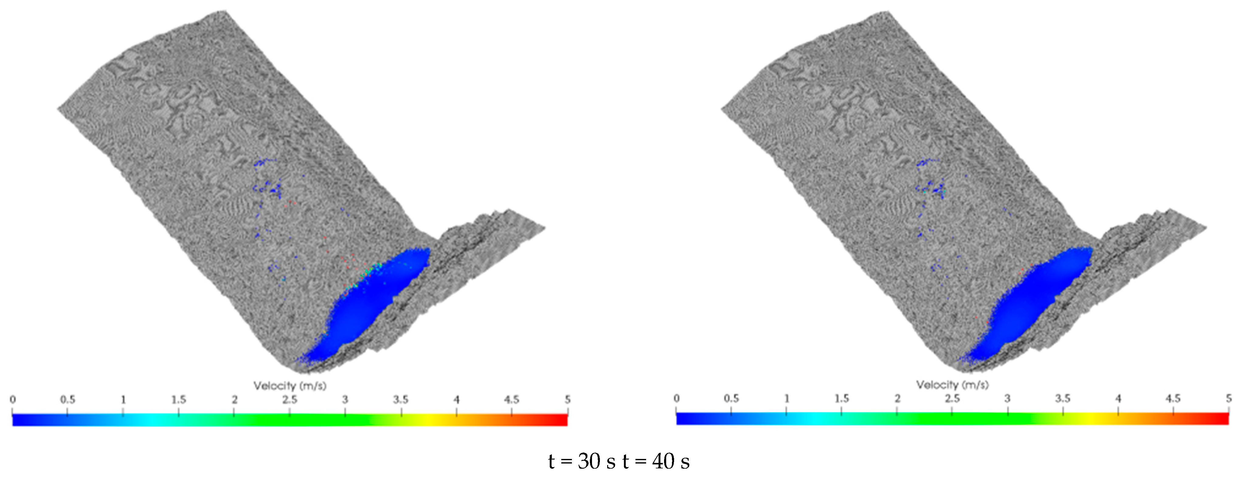
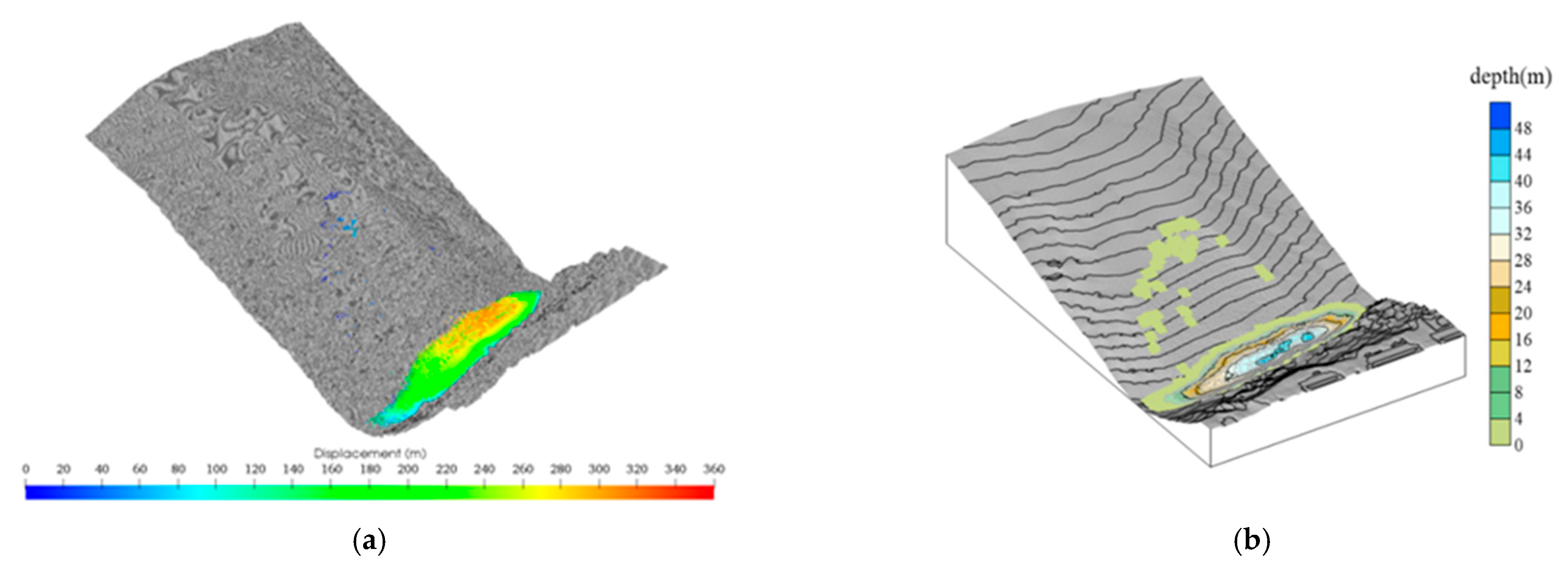
5.1. Ordinary Rainfall Conditions

The velocity evolution process of the landslide sliding under ordinary rainfall conditions is shown in Figure 17. The maximum velocity of the strong deformation zone in front of the landslide is more than 20 m/s, and it accumulates rapidly in the river channel after 30 s. In the process of the high-speed movement, the landslide body quickly disintegrates and blocks the river channel, and the accumulation body exceeds 500,000 m³.

To intuitively evaluate the material migration formed by the two landslides, the displacement distribution and accumulation depth of the landslide under the final form of accumulation are shown in Figure 18.

The maximum displacement of the landslide body exceeds 300 m, resulting in a wide scope of material migration. The maximum accumulation depth after sliding occurs in front of the landslide body that exceeds 31 m. The accumulation body formed in the river channel blocks the river channel, superimposing the blocking depth and the original terrain. The maximum blocking elevation in the river channel is 3090 m.

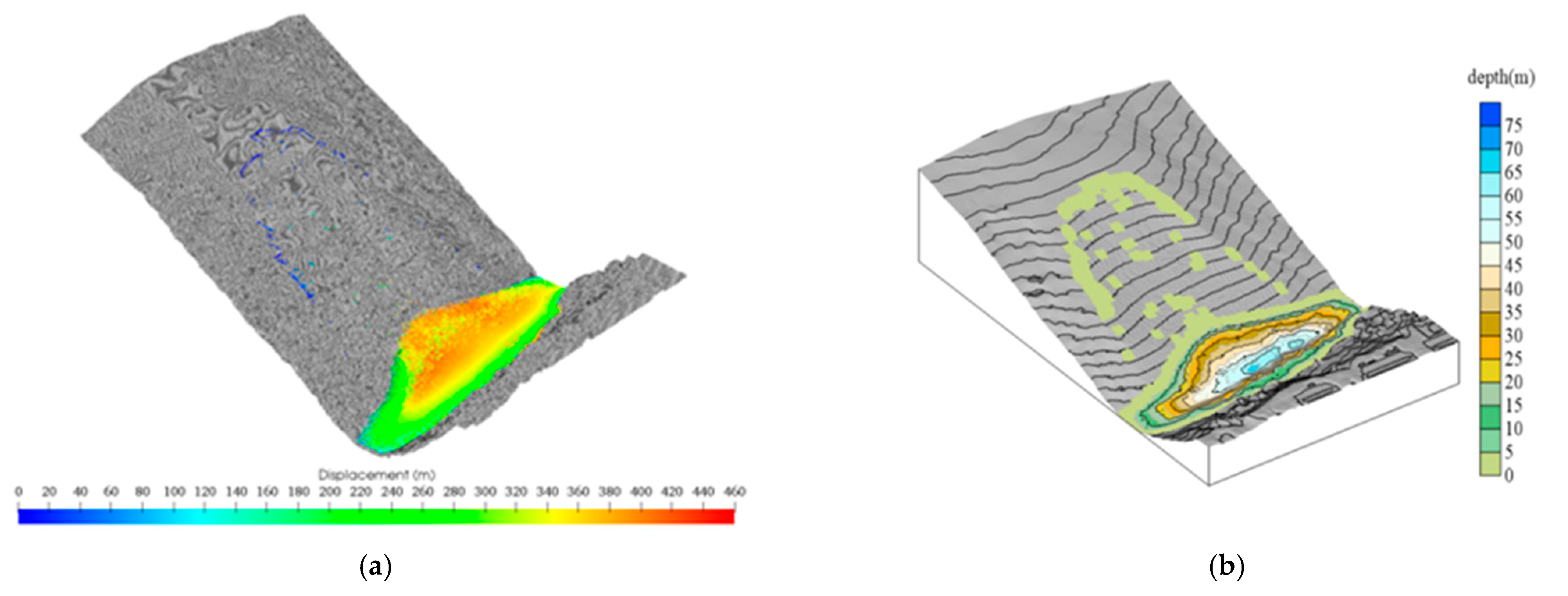
5.2. High-Intensity Rainfall Conditions

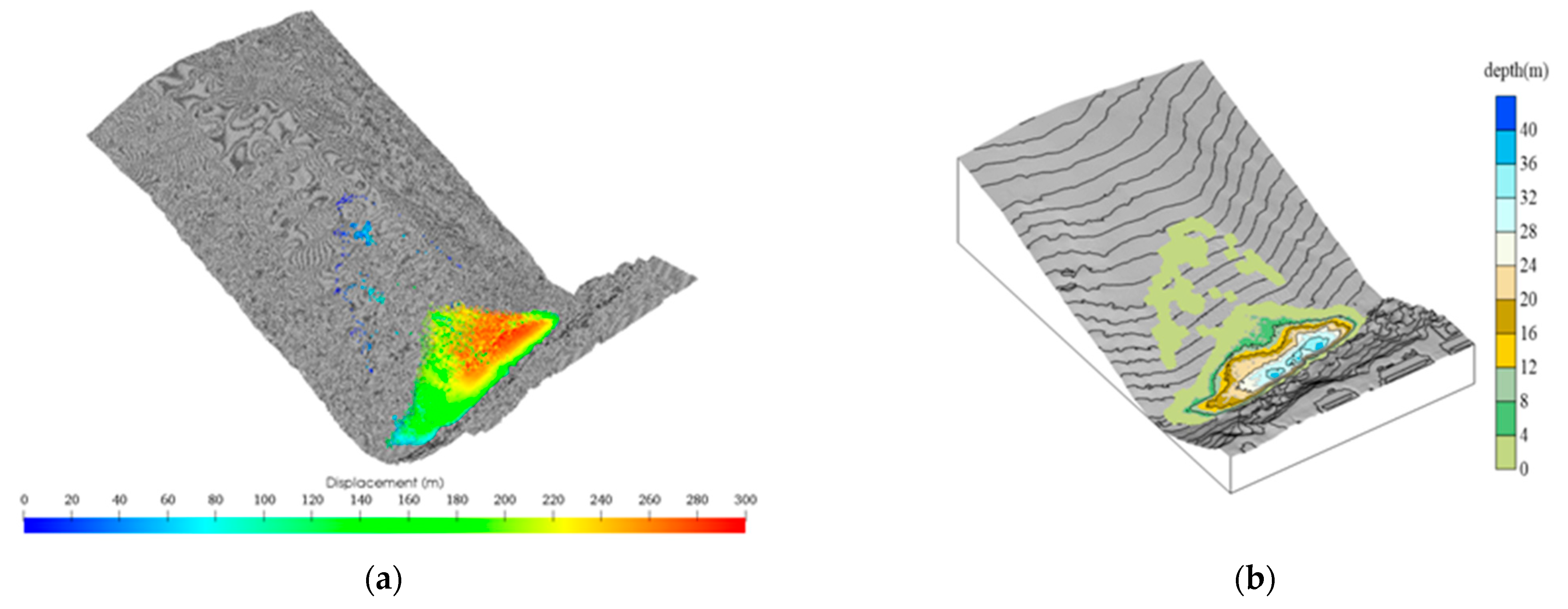
Under the high-intensity rainfall condition, the landslide occurred two times, both before and after sliding, and the velocity evolution process of the front and rear sliding of the landslide is shown in Figure 19 and Figure 20. According to the calculation results of Figure 19, it can be seen that the strong deformation zone in front of the landslide starts to slip first, the maximum movement speed after sliding initiates can exceed 25 m/s and it quickly accumulates in the river after 20 s. The slope collapses and blocks the river, and the volume of accumulation in the river exceeds 550,000 m³.

Taking the results of the sliding accumulation in the front of the landslide as the initial condition of the sliding in the back of the landslide, it can be seen from Figure 20 that during the calculation process, the overall weak deformation zone in the back of the landslide also experienced instability movement, with the maximum movement speed exceeding 36 m/s. Only a small amount of the landslide remained on the sliding surface, and the degree of river-blocking was expanded further. The total accumulation in the river channel was close to 1.6 million m³, which completely blocked the river channel.

To intuitively evaluate the material migration formed by the two landslides, the displacement distribution and accumulation depth of the landslide body after the final accumulation occurs are shown in Figure 21 and Figure 22.

The maximum displacement of the front part of the landslide is more than 360 m, and the maximum displacement of the whole sliding area is more than 460 m. At this time, the accumulation depth of the front sliding face of the landslide exceeds 40 m, and the river-blocking elevation reaches 3100 m. The accumulation depth of the subsequent weak deformation zone landslide after sliding occurs exceeds 65 m, and the accumulation body formed in the river channel is increased further. The movement distance of the landslide is farther, the accumulation in the river channel is larger and the final elevation of the river is also significantly increased.

According to the calculation results, the accumulation thickness of the landslide in the river and the range of the backwater elevation are predicted, and the range of the height of river-blocking after landslide instability is shown in Figure 23, which can provide a reference for secondary disaster prediction.

5.3. Discussion

Though the static-dynamic coupling method has been applied in this research and the single phase SPH method can be applied to simulate landslide river-blocking for large-scale landslide and smaller rivers, there are two obvious limitations in this research. Firstly, the landslide material is treated as single phase and the relative motion between the solid phase and liquid phase is ignored. Secondly, the water in the river is ignored because the stream discharge is small considering the volume of the landslide. This means though the simulation results can be applied to the analysis of the landslide motion and deposition process, they cannot reveal the dynamic mechanism of the landslide into river and wave generation process, and the final deposition simulation results may be biased. In our future research, the two-phase flow model will be introduced into SPH method to simulate the landslide blocking the river and swell propagation.

6. Conclusions

Aiming at the potential landslide river-blocking disaster, a combination of static analysis and dynamic simulation is proposed to analyze the risk of landslide river-blocking disaster. The novelty of this study is to combine FDM with SPH and take Bageduzhai landslide as an example to realize the simulation of landslide instability and movement process. Combined with the survey results of the landslide, the risk simulation analysis of river blocking is carried out, which is helpful to the prediction of the landslide blocking process.

The results of the field investigation show that the Bageduzhai landslide generally presents traction-falling landslide characteristics. Under natural conditions, the whole landslide presents a critical stable state, and there are strong and weak zones of deformation. There are obvious cracks at the trailing edge of the two regions, and there are obvious deformation and failure characteristics at the foot of the slope. The distribution characteristics of the stress and displacement fields under different rainfall conditions are obtained by static model simulation. The results show that instability failure can occur in the strong deformation zone under normal rainfall conditions. Under extreme rainfall conditions, instability failure may still occur in the weak deformation zone after the instability of the strong deformation zone.

According to the results of the static analysis, the position of the sliding surface is obtained, and on this basis, the SPH method is used to simulate and analyze river-blocking under both normal and extreme rainfall conditions. The results show that the unstable slope under normal rainfall conditions can block the river within 30 s, and the depth of river-blocking is 31 m. Under extreme rainfall conditions, the unstable slope in the strong deformation zone can block the river within 25 s, and the depth of river-blocking is 40 m. After the weak deformation zone is unstable, it can further block the river, and the depth of river-blocking can exceed 65 m, which causes great harm to the upstream and downstream towns and the roads on both sides of the river. Since the scouring effect of the river is not considered in the dynamic calculation process, the calculated elevation will increase within a small range.

The final research results show that the static–dynamic combination method can realize the quantitative evaluation of landslide river-blocking disaster risk, which provides a reference for the study of similar disasters.

References

1. Chen, X.Q.; Cui, P.; You, Y.; Cheng, Z.L.; Khan, A.; Ye, C.Y.; Zhang, S. Dam-break risk analysis of the Attabad landslide dam in Pakistan and emergency countermeasures. Landslides 2017, 14, 675–683. [Google Scholar] [CrossRef]
2. Arifianti, Y.; Pamela Iqbal, P.; Sumaryono, H.; Omang, A.; Lestiana, H. Susceptibility Assessment of Earthquake-induced Landslides: The 2018 Palu, Sulawesi Mw 7.5 Earthquake, Indonesia. Rud. Geol. Naft. Zb. 2023, 38, 43–54. [Google Scholar] [CrossRef]
3. Sincic, M.; Gazibara, S.B.; Krkac, M.; Arbanas, S.M. Landslide susceptibility assessment of the City or Karlovac using the bivariate statistical analysis. Rud. Geol. Naft. Zb. 2022, 37, 149–170. [Google Scholar] [CrossRef]
4. Wang, L.; Wu, C.; Yang, Z.; Wang, L. Deep learning methods for time-dependent reliability analysis of reservoir slopes in spatially variable soils. Comput. Geotech. 2023, 159, 105413. [Google Scholar] [CrossRef]
5. Chen, B.; Shui, W.; Liu, Y.; Deng, R. Analysis of Slope Stability with Different Vegetation Types under the Influence of Rainfall. Forests 2023, 14, 1865. [Google Scholar] [CrossRef]
6. Zhang, W.; Wu, C.; Tang, L.; Gu, X.; Wang, L. Efficient time-variant reliability analysis of Bazimen landslide in the Three Gorges Reservoir Area using XGBoost and LightGBM algorithms. Gondwana Res. 2023, 123, 41–53. [Google Scholar] [CrossRef]
7. Costa, J.E.; Schuster, R.L. The formation and failure of natural dams. Geol. Soc. Am. Bull. 1988, 100, 1054–1068. [Google Scholar] [CrossRef]
8. Wang, P.; Chen, J.; Dai, F.; Long, W.; Xu, C.; Sun, J.; Cui, Z. Chronology of relict lake deposits around the Suwalong paleolandslide in the upper Jinsha River, SE Tibetan Plateau: Implications to Holocene tectonic perturbations. Geomorphology 2014, 217, 193–203. [Google Scholar] [CrossRef]
9. Bao, Y.; Sun, X.; Zhou, X.; Zhang, Y.; Liu, Y. Some numerical approaches for landslide river blocking: Introduction, simulation, and discussion. Landslides 2021, 18, 3907–3922. [Google Scholar] [CrossRef]
10. Bao, Y.; Zhai, S.; Chen, J.; Xu, P.; Sun, X.; Zhan, J.; Zhang, W.; Zhou, X. The evolution of the Samaoding paleolandslide river blocking event at the upstream reaches of the Jinsha River, Tibetan Plateau. Geomorphology 2020, 351, 106970. [Google Scholar] [CrossRef]
11. Ermini, L.; Gasagli, N. Prediction of the behaviour of landslide dams using a geomorphological dimensionless index. Earth Surf. Process. Landf. 2003, 28, 31–47. [Google Scholar] [CrossRef]
12. Dal Sasso, S.F.; Sole, A.; Pascale, S.; Sdao, F.; Bateman Pinzon, A.; Medina, V. Assessment methodology for the prediction of landslide dam hazard. Nat. Hazards Earth Syst. Sci. 2014, 14, 557–567. [Google Scholar] [CrossRef]
13. Stefanelli, C.T.; Segoni, S.; Casagli, N.; Catani, F. Geomorphic indexing of landslide dams evolution. Eng. Geol. 2016, 208, 1–10. [Google Scholar] [CrossRef]
14. Griffiths, D.V.; Lane, P.A. Slope stability analysis by finite elements. Geotechnique 1999, 49, 387–403. [Google Scholar] [CrossRef]
15. Dawson, E.M.; Roth, W.H.; Drescher, A. Slope stability analysis by strength reduction. Geotechnique 1999, 49, 835–840. [Google Scholar] [CrossRef]
16. Shi, G.H.; Goodman, R.E. 2 dimensional discontinuous deformation analysis. Int. J. Numer. Anal. Methods Geomech. 1985, 9, 541–556. [Google Scholar] [CrossRef]
17. Wang, W.; Chen, G.-Q.; Zhang, H.; Zhou, S.-H.; Liu, S.-G.; Wu, Y.-Q.; Fan, F.-S. Analysis of landslide-generated impulsive waves using a coupled DDA-SPH method. Eng. Anal. Bound. Elem. 2016, 64, 267–277. [Google Scholar] [CrossRef]
18. Zhang, H.; Chen, G.; Zheng, L.; Han, Z.; Zhang, Y.; Wu, Y.; Liu, S. Detection of contacts between three-dimensional polyhedral blocks for discontinuous deformation analysis. Int. J. Rock Mech. Min. Sci. 2015, 78, 57–73. [Google Scholar] [CrossRef]
19. Wu, J.-H.; Chen, C.-H. Application of DDA to simulate characteristics of the Tsaoling landslide. Comput. Geotech. 2011, 38, 741–750. [Google Scholar] [CrossRef]
20. Gingold, R.A.; Monaghan, J.J. Smoothed particle hydrodynamics: Theory and application to non-spherical stars. Mon. Not. R. Astron. Soc. 1977, 181, 375–389. [Google Scholar] [CrossRef]
21. Lucy, L.B. A numerical approach to the testing of the fission hypothesis close binary star formation. Astron. J. 1977, 82, 1013–1024. [Google Scholar] [CrossRef]
22. Bui, H.H.; Fukagawa, R.; Sako, K.; Ohno, S. Lagrangian meshfree particles method (SPH) for large deformation and failure flows of geomaterial using elastic-plastic soil constitutive model. Int. J. Numer. Anal. Methods Geomech. 2008, 32, 1537–1570. [Google Scholar] [CrossRef]
23. Bui, H.H.; Fukagawa, R.; Sako, K.; Wells, J.C. Slope stability analysis and discontinuous slope failure simulation by elasto-plastic smoothed particle hydrodynamics (SPH). Geotechnique 2011, 61, 565–574. [Google Scholar] [CrossRef]
24. Li, L.; Wang, Y.; Zhang, L.; Choi, C.; Ng, C.W.W. Evaluation of Critical Slip Surface in Limit Equilibrium Analysis of Slope Stability by Smoothed Particle Hydrodynamics. Int. J. Geomech. 2019, 19, 04019032. [Google Scholar] [CrossRef]
25. Liang, H.; He, S.; Chen, Z.; Liu, W. Modified two-phase dilatancy SPH model for saturated sand column collapse simulations. Eng. Geol. 2019, 260, 105219. [Google Scholar] [CrossRef]
26. Liang, H.; He, S.; Jiang, Y. Study of the Dilatancy/Contraction Mechanism of Landslide Fluidization Behavior Using an Initially Saturated Granular Column Collapse Simulation. Water Resour. Res. 2021, 57, e2020WR028802. [Google Scholar] [CrossRef]
27. Liang, H.; He, S.; Lei, X.; Bi, Y.; Liu, W.; Ouyang, C. Dynamic process simulation of construction solid waste (CSW) landfill landslide based on SPH considering dilatancy effects. Bull. Eng. Geol. Environ. 2019, 78, 763–777. [Google Scholar] [CrossRef]
28. Liang, H.; He, S.; Liu, W. Dynamic simulation of rockslide-debris flow based on an elastic-plastic framework using the SPH method. Bull. Eng. Geol. Environ. 2020, 79, 451–465. [Google Scholar] [CrossRef]
29. Zhao, T.; Dai, F.; Xu, N.-W. Coupled DEM-CFD investigation on the formation of landslide dams in narrow rivers. Landslides 2017, 14, 189–201. [Google Scholar] [CrossRef]
30. Wang, W.; Chen, G.; Zhang, Y.; Zheng, L.; Zhang, H. Dynamic simulation of landslide dam behavior considering kinematic characteristics using a coupled DDA-SPH method. Eng. Anal. Bound. Elem. 2017, 80, 172–183. [Google Scholar] [CrossRef]
31. Liu, W.; He, S.-M.; OuYang, C.-J. Dynamic process simulation with a Savage-Hutter type model for the intrusion of landslide into river. J. Mt. Sci. 2016, 13, 1265–1274. [Google Scholar] [CrossRef]
32. Liu, W.; He, S. A two-layer model for simulating landslide dam over mobile river beds. Landslides 2016, 13, 565–576. [Google Scholar] [CrossRef]
33. Bao, Y.; Su, L.; Chen, J.; Ouyang, C.; Yang, T.; Lei, Z.; Li, Z. Dynamic process of a high-level landslide blocking river event in a deep valley area based on FDEM-SPH coupling approach. Eng. Geol. 2023, 319, e2020WR028802. [Google Scholar] [CrossRef]
34. Feng, R.; Fourtakas, G.; Rogers, B.D.; Lombardi, D. Two-phase fully-coupled smoothed particle hydrodynamics (SPH) model for unsaturated soils and its application to rainfall-induced slope collapse. Comput. Geotech. 2022, 151, 104964. [Google Scholar] [CrossRef]
Figure 1. Location map of the study area.
Water 15 03739 g001
Figure 2. Geological sketch and spatial location of the Bageduzhai landslide.
Water 15 03739 g002
Figure 3. Strong and weak deformation zones.
Water 15 03739 g003
Figure 4. Surface loess and Quaternary ice-water accumulation gravel soil (middle and rear part of landslide).
Water 15 03739 g004
Figure 5. Failure characteristics of the strong deformation zone in front of the landslide.
Water 15 03739 g005
Figure 6. Failure characteristics of the weak deformation zone behind the landslide.
Water 15 03739 g006
Figure 7. Particle size distribution and physical flume model experiment. (a) The particle grading diagram of the landslide; (b) the channel of experiment and numerical simulation.
Water 15 03739 g007aWater 15 03739 g007b
Figure 8. Comparison of the indoor physical model experiment and the numerical simulation at 500 ms, 900 ms and 1400 ms.
Water 15 03739 g008
Figure 9. FLAC calculation cycle diagram.
Water 15 03739 g009
Figure 10. The topographic map and the stability analysis calculation model of the landslide. (a) Topographic map of the landslide area; (b) the numerical model of the stability analysis.
Water 15 03739 g010
Figure 11. Characteristics of the landslide stress field in the strong deformation zone under ordinary rainfall conditions. (a) Maximum principal stress; (b) Minimum principal stressss; (c) Maximum principal stress of section; (d) Minimum principal stress of section.
Water 15 03739 g011
Figure 12. Deformation characteristics of landslides in strong deformation zones under ordinary rainfall conditions. (a) Total displacement; (b) Horizontal displacement; (c) Total displacement of section; (d) Horizontal displacement of profile.
Water 15 03739 g012
Figure 13. Characteristics of the landslide stress field in the weak deformation zone under extreme rainfall conditions. (a) Maximum principal stress; (b) Minimum principal stressss; (c) Maximum principal stress of section; (d) Minimum principal stress of section.
Water 15 03739 g013
Figure 14. Deformation characteristics of landslides in weak deformation zones under extreme rainfall conditions. (a) Total displacement; (b) Horizontal displacement; (c) Total displacement of section; (d) Horizontal displacement of profile.
Water 15 03739 g014
Figure 15. Potential sliding surface penetration of landslides under different conditions.
Water 15 03739 g015
Figure 16. The dynamic process calculation model of the landslide. (a) Three-dimensional physical model of landslide; (b) original landform of landslide.
Water 15 03739 g016
Figure 17. Evolutionary process of the sliding velocity in front of the landslide (Ordinary Rainfall Conditions).
Water 15 03739 g017aWater 15 03739 g017b
Figure 18. The final simulation results of the landslide in ordinary rainfall condition. Sliding displacement of the landslide mass. (a) Sliding displacement of the landslide mass; (b) accumulation depth of the landslide mass.
Water 15 03739 g018
Figure 19. Evolutionary process of the sliding velocity in front of the landslide (High-Intensity Rainfall Conditions).
Water 15 03739 g019aWater 15 03739 g019b
Figure 20. Evolutionary process of the sliding velocity behind the landslide.
Water 15 03739 g020aWater 15 03739 g020b
Figure 21. The simulation results of the first landslide in high-intensity rainfall condition. (a) Displacement after sliding (front strong deformation zone); (b) accumulation depth after sliding.
Water 15 03739 g021
Figure 22. The simulation results of the second landslide in high-intensity rainfall condition. (a) Displacement after all sliding (before and after landslide); (b) accumulation depth after all sliding.
Water 15 03739 g022
Figure 23. The range of the height of river-blocking after the landslide instability failure occurs.
Water 15 03739 g023