Article

Significant Dynamic Disturbance of Water Environment Quality in Urban Rivers Flowing through Industrial Areas

1
Hubei Key Laboratory of Resource and Ecological Environment Geology, Wuhan 430100, China
2
Geophysical Exploration Brigade of Hubei Geological Bureau, Wuhan 430100, China
3
College of Landscape Architecture, Sichuan Agricultural University, Chengdu 611130, China
4
School of Art and Design, Xihua University, Chengdu 610039, China
5
Tourism School, Chengdu Polytechnic, Chengdu 610093, China
6
Faculty of Engineering, China University of Geosciences (Wuhan), Wuhan 430100, China
7
Sichuan Yuze (Xscape) Landscape Planning and Design Co., Ltd., Chengdu 610093, China
*
Authors to whom correspondence should be addressed.
Water 2023, 15(20), 3640; https://doi.org/10.3390/w15203640
Submission received: 25 August 2023 / Revised: 4 October 2023 / Accepted: 10 October 2023 / Published: 17 October 2023

Abstract

:
The urban water environment is seriously affected by human activities. Rivers in highly industrialized areas, which often carry various types of industrial pollutants, such as metals and nutrients, are especially affected. In this study, the water quality of the Pi River, an industrial base that flows through Chengdu, a large city in Southwest China, was tested for one year. Heavy metal concentrations in the water, sediment, and macrobenthic and algal communities in the river were examined. The water pollution index (WPI) and trophic level index (TLI) were employed to measure the water pollution degree and eutrophication status, respectively. The Shannon—Wiener index (H’) and Margalef’s index (dM) were determined to represent the diversity and richness of macroinvertebrates. The principal component analysis (PCA) was employed to define the main heavy metal influencing factors in the Pi River. Our study showed that the eutrophication status increased with spatial change, and the eutrophication status was the most serious in the downstream reach, which was moderately eutrophic. The water body of the Pi River was seriously polluted by heavy metals, and the content of chromium (Cr) in the sediment and cadmium (Cd) in the water/sediment was far beyond the prescribed limit. In addition, we found that Cd had a serious impact on both the benthic and algal communities, and the benthic community structure was completely changed, destroying the original aquatic environment. We explored the mechanisms of the influence of Cd on aquatic fauna, and this information is of great significance for the future conservation of industrial urban rivers. In this study, the spatial–temporal variations in water quality and aquatic communities revealed the pollution status of a river flowing through industrial areas, which provided a basis for future river conservation and restoration.

Graphical Abstract

1. Introduction

Urban water is increasingly strained due to rapid urbanization, resulting in water quality deterioration in freshwater ecosystems, habitat degradation, and a significant decline in biodiversity. Water quality deterioration is mainly manifested as black and odorous water, eutrophication, and metal pollution, which are the main pollution phenomena of urban rivers in developing countries [1,2,3,4].
The outbreak of water eutrophication mostly results from the continual increase in nutrient elements in water and is closely related to the population density and quantity of aquatic algae. Nitrogen (N) and phosphorus (P) from agricultural nonpoint source pollution, farm runoff, and leachate pollution from solid wastes are limiting factors affecting the various components needed for algal reproduction [5]. The organic pollutants in eutrophic water can seriously endanger water safety and cause an imbalance in species structures in river ecosystems. Algal blooms obscure water bodies and weaken the photosynthesis of aquatic plants, thus seriously affecting the self-purification ability of aquatic ecosystems. When algae are decomposed by microorganisms, a large amount of dissolved oxygen is consumed, and in serious cases, anaerobic conditions occur and produce an odor [6]. The competitive ability of the algae population to the environment is obviously different, and the proportion of nutrients needed for growth varies. Seasonal variations in the N/P ratio can change the limiting characteristics of nutrients in water, and N/P represents one of the key factors regulating algal growth alternation. This also reveals the impact of nutrient increases on the water nutritional environment. The nutrient level increases with decreasing N/P [7]. The organic matter greatly increases in eutrophic water, causing harmful pathogens and algal toxins and endangering the safety of drinking water [8]. Therefore, the potential risks of river eutrophication and its accumulation of toxic chemicals in river ecosystems should be studied in detail.
Heavy metals are highly toxic, persistent, and refractory environmental pollutants that exist in aquatic environments and can be absorbed by river organisms. Heavy metal pollution in water caused by accelerated industrialization and urbanization has become one of the world’s environmental problems [9,10]. River sediment is an important part of urban river ecosystems. Heavy metals enter the sediment through flocculation or precipitation. However, heavy metals in sediments can be rereleased into water after being affected by changes in the overlying water environment and can become potential pollution sources [11]. Metals in water and sediment are gradually transferred and re-enriched up the food chain through absorption by organisms [12]. As an important component of aquatic ecosystems, macrobenthos are widely used in water environment monitoring and ecosystem health evaluation due to their characteristics of wide distribution, long life cycle, poor mobility, limited range of activities, and sensitivity to environmental changes [13]. The dynamics of community structure when water pollution is more serious are due to the different tolerances of macrobenthos, so they have a certain indication of heavy metal pollution in rivers [14]. Studies have shown that heavy metal content in sediments is significantly correlated with the diversity of the benthic community structure, and the sizes of EPT (Ephemeroptera, Plecoptera, and Trichoptera) populations at sites polluted by heavy metals are significantly higher than those at reference sites [15]. The effects of metals on benthic and fish community composition are significant even at low pollution levels [16]. Certain heavy metals are concentrated in macrobenthic invertebrates due to their breathing and feeding behavior and can cause negative effects such as indigestion, reduced breathing, and slow movement [17]. Heavy metals also affect the growth of fish, and studies have found that heavy metal elements such as Cd and Hg easily combine with the smell and taste neurons of fish, producing inhibitory effects [18]. Therefore, the potential risks of eutrophication and heavy metal accumulation in urban rivers should be further studied. Most studies on the pollution of urban rivers have focused on the eutrophication of water caused by nutrients or the hazard of metals in water; however, research on the relationship between them has been insufficient.
Chengdu is a megacity in which nearly 20 million citizens live, and it is the electronics industrial center of Southwest China. In recent years, environmental pressure has increased with the industrial development of Chengdu. The Xindu and Jintang Districts along the Pi River have always been important chemical, metallurgical, and building material bases in Chengdu, with numerous industrial activities and frequent human activities in the area. The Pi River is one of the water channels for Dujiangyan, and the groundwater of the Pi River is the alternate water source for Chengdu [19]. The improvement of water quality and the restoration of the water environment are of great significance to the improvement of the living quality and water safety of residents in the region.

2. Materials and Methods

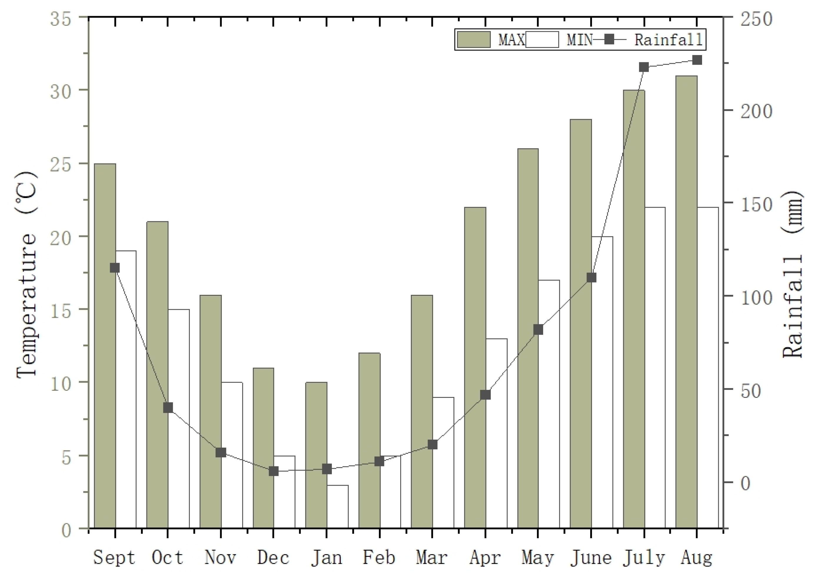
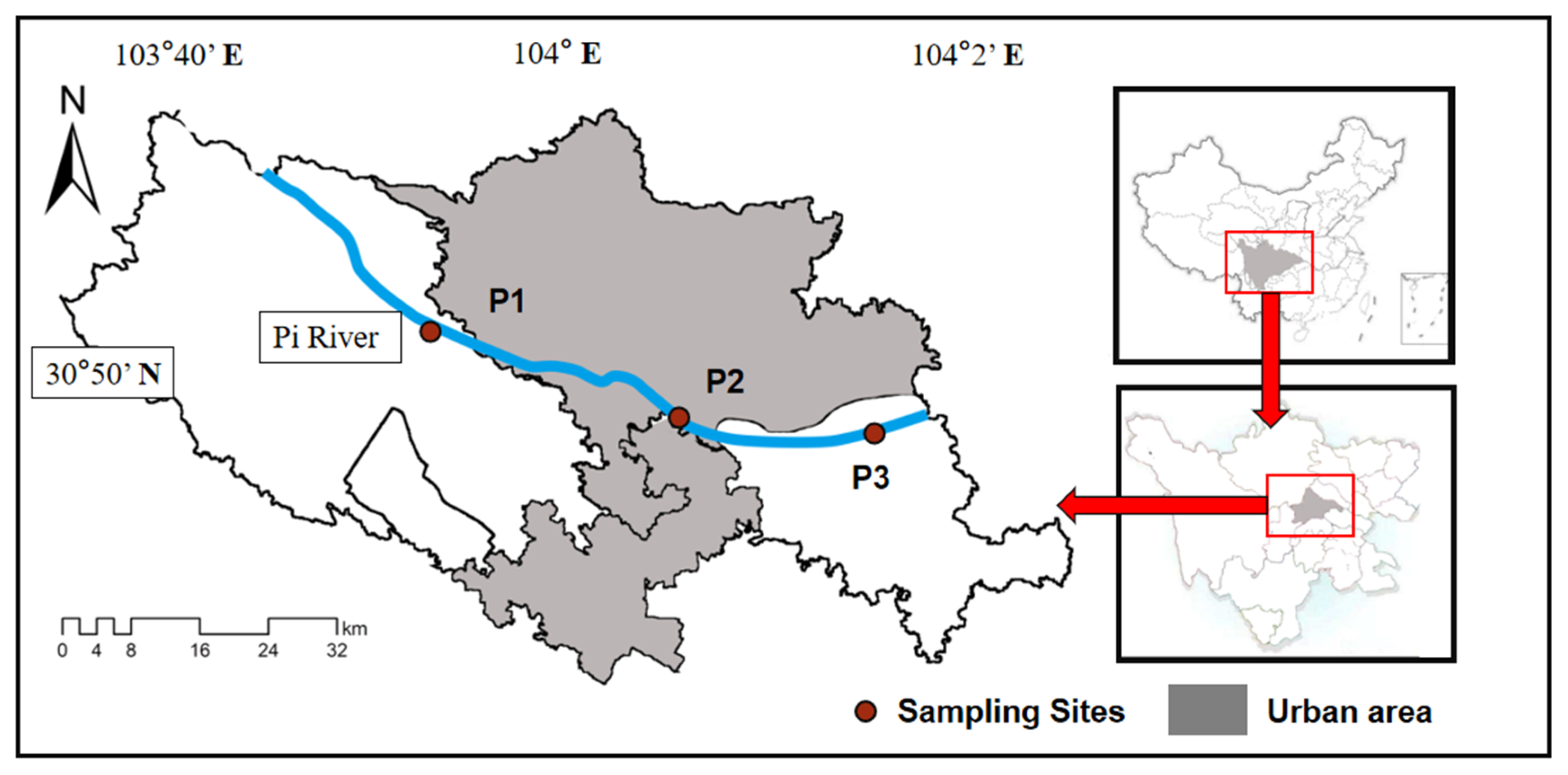
2.1. Study Area Description and Sampling Sites

The studied river is located in Chengdu, Sichuan, southwest China. The average altitude of Chengdu is 750 m, and the temperature ranges from 2 to 31 °C (Figure 1). Based on the data of the Meteorological Bureau of Chengdu, to reflect the seasonality of river hydrology, the authors classified spring (from March to May), summer (from June to August), autumn (from September to November), and winter (from December to February), and the average season lasted approximately three months.
The water supply of the Chengdu area is mainly provided by the Minjiang River from Dujiangyan. The Pi River flows through the northern part of the main city of Chengdu, with an irrigated area of 1973.3 hm2 and an annual flow of approximately 26.4 m3 s−1. To reflect the spatial difference, we selected three representative sampling points in the upstream reach (P1), in the middle (P2), and in the downstream reach (P3) of the Pi River (Figure 2). P1 was far from the areas with intensive human activities, and human activities have little influence on the river environment. P2 was located in the central area of the city in an urban park surrounded by traffic arteries and distribution centers of the building materials industry. P3 was outside the main urban area of Chengdu, and the surrounding land use is mostly used for agricultural activities. The distance between the sampling points was 15–20 km, effectively highlighting the difference in spatial water quality.

2.2. Water Sampling

The samples were collected on sunny days monthly within one year (from September 2020 to August 2021). The sampling interval was more than 20 days. Algae and benthic samples were collected quarterly (seasonally). All the water sample collection procedures and methods followed the standard methods issued by the Ministry of Ecology and Environment of the People’s Republic of China (abbreviated as MEEC) [20]. Before sampling, the sampler and the plastic bottle were rinsed several times with water from the sampling site to avoid cross-contamination. The water samples were well preserved in 500–1000 mL plastic bottles, stored in a refrigerator, and immediately sent to a professional laboratory. Zooplankton samples were assembled, and Lugol’s iodine solution (Shanghai Xinyu Biotechnology Co., Shanghai, China) was used for immobilization before testing in the laboratory. The macroinvertebrate samples were mainly sampled by kicking nets, with a size of 1 m × 1 m and a mesh size of 0.5 mm, and each section was randomly sampled 5–10 times. A 40-mesh sample screen was then used for screening, stone brushing was used for collection at shoals, and digging was carried out in deeper places. The samples were mixed with at least three to five quadrat samples. Each sampling area was greater than 1 m2 and penetrated at least 20 cm of sediment. The collected macroinvertebrates were fixed using a formic acid solution, brought back to the laboratory, and then transferred into alcohol for long-term preservation. Sediment sampling was performed by taking river sediment at each site using a hand shovel, and the samples were mixed in at least three quadrants (1.5 kg, sample: 25 cm × 25 cm, depth 5–10 cm) [21].

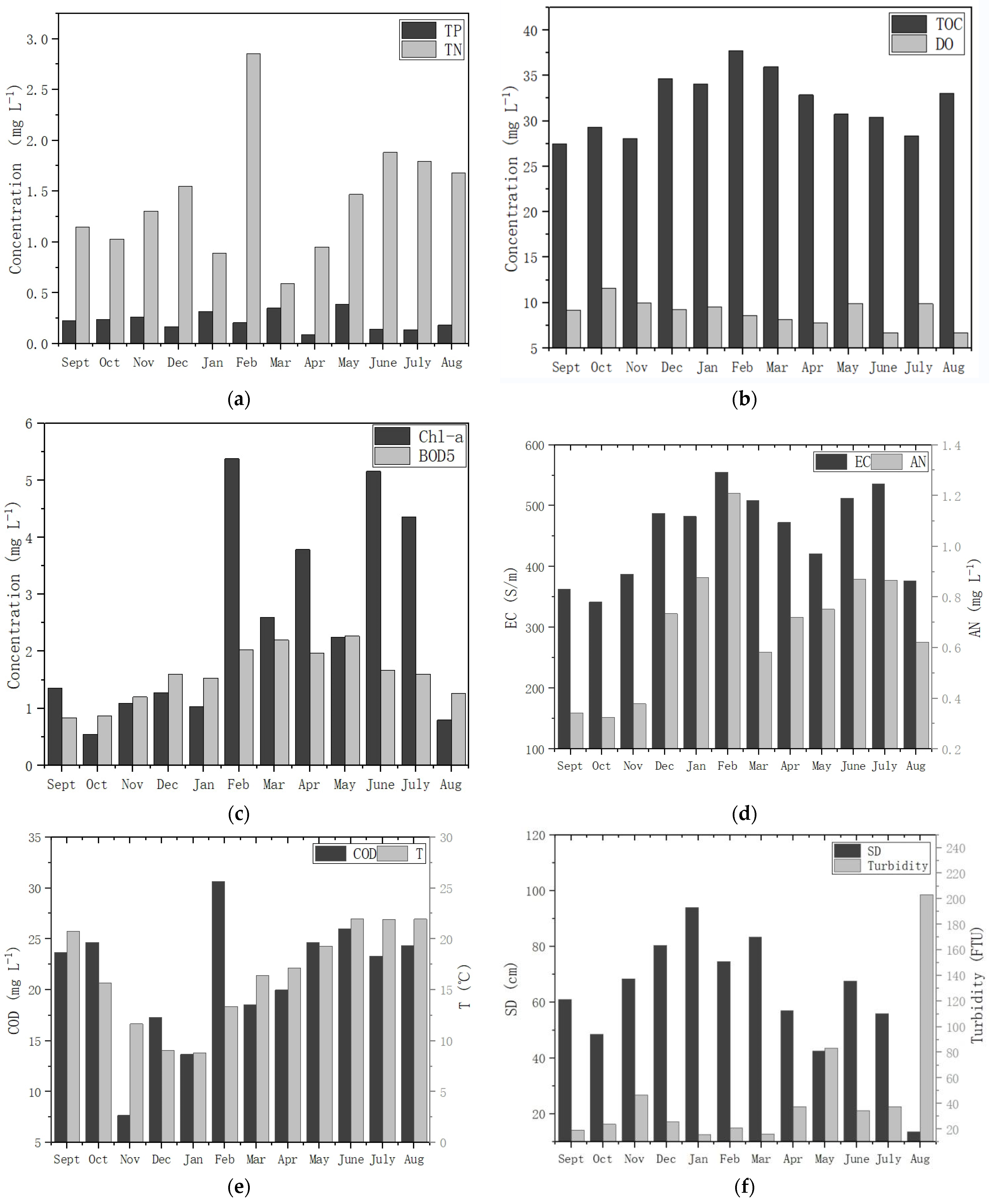
2.3. Measurement of Water Quality Parameters

The water quality constituents included total organic carbon (TOC), total phosphorus (TP), total nitrogen (TN), five-day biochemical oxygen demand (BOD5), ammonia nitrogen (AN), chlorophyll a (Chl-a), and chemical oxygen demand (COD). The water quality parameters were measured according to the standard methods of the MEEC [20]. The temperature (T), turbidity (Hach 2100Q, Loveland, CO, USA), diaphaneity (Secchi depth, SD), dissolved oxygen (DO) concentration (Hach HQ1130, Loveland, CO, USA), and pH value (Smart Sensor PH8008, Houston, TX, USA) of the river water were measured at the scene. The concentrations of the heavy metals lead (Pb), chromium (Cr), cadmium (Cd), arsenic (As), mercury (Hg), manganese (Mn), iron (Fe), and copper (Cu) were determined according to the methods introduced by the standard methods of the MEEC (2002) using a spectrophotometer (SHKTYQ 752N754, Shanghai, China) and measured according to previous standards [22].

2.4. Environmental Quality Assessment Method of Surface Water

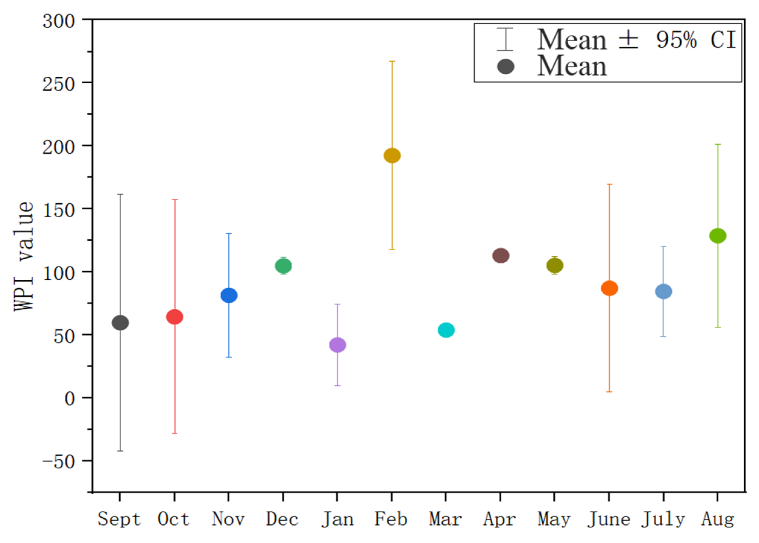
2.4.1. Water Pollution Index

The water pollution index (WPI) is a metric that has advantages in comparing the pollution degree of different water quality parameters, water quality classifications, and water quality quantitative evaluations [23]. In addition, it refers to the water pollution limits and reflects the temporal and spatial variations in evaluating water environmental quality. The calculation process is simple [24,25]. The WPI divides water quality into six grades (Table 1). The lower the WPI value, the better the water quality. If the measured value is less than the V limit value, the WPI is calculated using the following formula.
W P I i = W P I l i + W P I h i W P I l i C h i C l i C i C l i C l ( i ) < C ( i ) C h ( i )
where C(i) is the detected value of the water quality index of i, Cl(i) is the lowest value for class i, Ch(i) is the highest value of class i, WPIl(i) is the index value corresponding to the minimum value of class i, WPIh(i) is the index value corresponding to the highest value of class i, and WPI(i) is the index value corresponding to i. The calculation formula of the WPI value exceeding the Class Ⅴ standard value is as follows.
W P I i = 100 + C i C 5 i C 5 i 40
where C5(i) is the Class Ⅴ standard value of i in GB 3838-2002. The water pollution index value of the final sampling section is determined as the maximum value.
W P I = M A X ( W P I ( i ) )

2.4.2. Trophic Level Index

The TLI was modified from Carlson’s trophic state index (TSIM) and the trophic state classification for the detection of water quality in lakes and rivers [26]. The equation of the trophic level index is as follows.
T L I ( ) = n = 1 m W n T L I n
In the formula, TLI () is the comprehensive nutrient state index of the water body, Wn is the weight of the eutrophication status index of j, and TLI (n) is the eutrophication status index of n. The normalized Wn of n can be measured as follows with Chl-a as the reference index.
W n = r i n 2 n = 1 m r i n 2
where rin is the correlation coefficient between n and the reference indicator Chl-a and m is the value of the participants in the eutrophication status assessment. The nutritional status of the other indexes is calculated using the following formulas.
T L I ( C h l a ) = 10 × ( 2.5 + 1.086 ln C h l a ) T L I ( T P ) = 10 × ( 9.436 + 1.624 ln T P ) T L I ( T N ) = 10 × ( 5.453 + 1.694 ln T N ) T L I ( S D ) = 10 × ( 5.118 1.94 ln S D ) T L I ( C O D ) = 10 × ( 0.62 + 2.56 ln C O D )
To present the state of eutrophication of the Pi River, we graded the nutritional situation and evaluation of the aquatic environment by using a rating range from 0 to 100. It was useful to set a eutrophication assessment standard in different regions to aid in setting target nutrient concentrations to reach desirable trophic states (Table 2).

2.4.3. Measurement of the Diversity and Richness of Benthic Macrobenthos

The Shannon–Wiener diversity index (H’) (7) and Margalef’s richness index (dM) (8) were used to infer the level of benthic biodiversity of the Pi River.
H = i = 1 S ( n i N ) log 2 ( n i N )
d M = S 1 ln N
where ni is the value of the individuals of the ith species, N is the total number of samples, and S is the value of the species.
The evaluation criteria of the Shannon–Wiener diversity index (H’) are as follows (Table 3).
The evaluation criteria of Margalef’s richness index (dM) are as follows (Table 4).

2.5. Statistical Analysis

The Shapiro–Wilk test was conducted to test for normality in the water quality index data before the statistical analysis. The Spearman correlation test was used for all the parameters. The spatial and temporal heterogeneity and eutrophication of the river water quality were analyzed using the WPI and TLI, respectively. The principal component analysis (PCA) was performed using the IBM SPSS 20.0 software, which was used to determine the main influential factors of metals in the Pi River.

3. Results

3.1. Temporal–Spatial Variation in the Water Quality Index

The results of the environmental factors and water quality indicators of the Pi River after one year of water quality testing, and the range and mean values of these parameters, are included in Table 5. The annual changes in each index are shown in Figure 3. The TN and WPI had similar variation trends, both reaching a peak value (TN was 2.86 mg L−1 and WPI was 170.53) in February, but the TN plummeted to 0.59 mg L−1 in March. The TN was relatively stable in the mean flow period (spring and autumn) and slightly higher in the wet season (summer). T was negatively correlated with the SD and DO (p < 0.01, r2 = −538 **; p < 0.01, r2 = −572 **). The SD had the opposite trend of turbidity, with turbidity reaching a peak of 205 in August and the SD reaching a minimum value of 4 cm (Figure 3). Due to waterlogging in the Xindu District in August, the river received a large amount of sediment and pollutants, leading to river turbidity. The two parameters were negatively correlated (p < 0.01, r2 = −702 **). The TN was significantly positively correlated with the TP, AN, COD, Chl-a, and TOC (p < 0.01). The BOD5 and Chl-a both reached their peak values in winter and had a significant positive correlation (r2 = 432 **, r2 = 487 **). DO was relatively stable but had a downward trend in the wet season (summer), which was different from the TOC (p < 0.01, r2 = −612 **). The variation trends of AN and the COD were similar to those of the TN and TP, both reaching their peak values in February, and the two indexes showed extremely significant positive correlations (r2 = 432 **, r2 = 534 **).
The average WPI of the Pi River was 93.16 (n = 36), and 21 inferior V sections with WPI scores higher than 100 accounted for 58.33%, indicating serious pollution. Eleven sections were classified as class III or below, accounting for 30.55%. Overall, the water quality was acceptable and relatively clean. The monthly mean value was highest in February (WPI = 192.53) and lowest in January (WPI = 42.12). Among all the seasons, the WPIs in summer and winter were significantly higher. The highest WPI value in winter was 113.17, and the lowest WPI value in autumn was 68.56 (Figure 4).

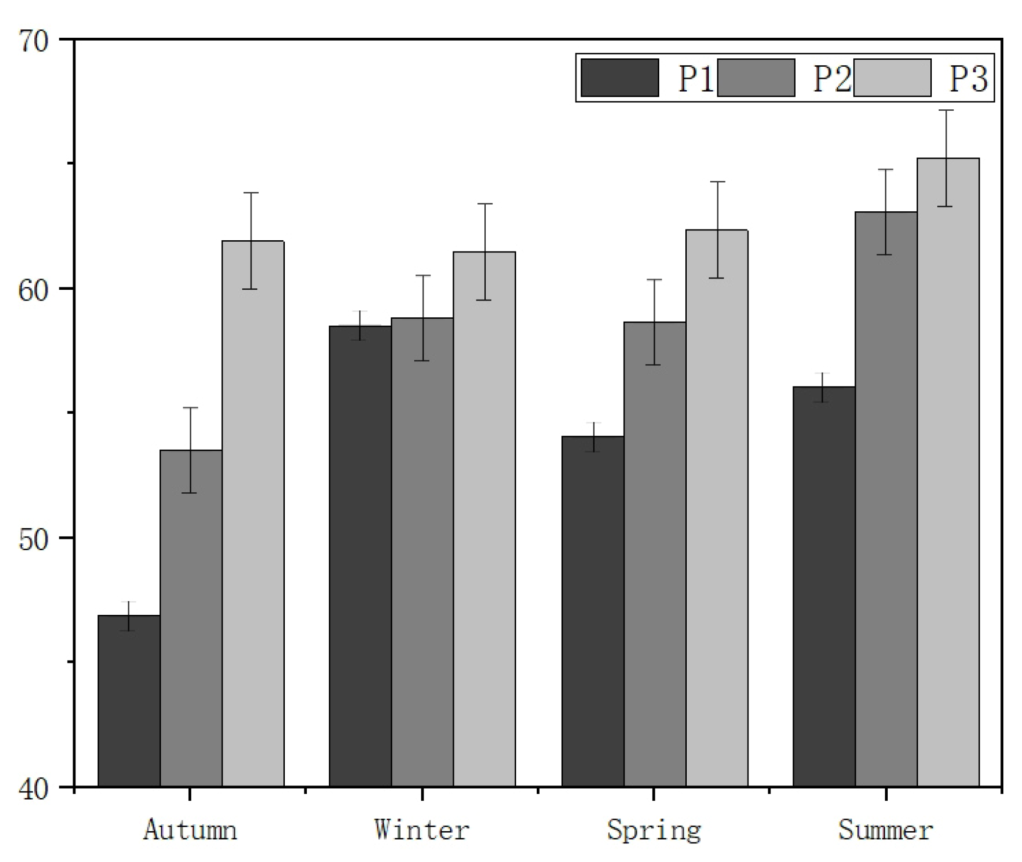
3.2. Spatiotemporal Variations in the TLI (∑)

Based on Chl-a as the leading factor evaluation parameter, the TN, TP, COD and SD, which were significantly correlated with Chl-a, were selected to calculate the TLI (∑) eutrophication state index. The spatiotemporal changes in the eutrophication state index in the season of the Pi River were obtained, as shown in Figure 5. The TLI (∑) in P1 of the river was the lowest (mean 53.89), followed by P2 (mean 58.53). P3 was the highest (mean 62.76). The annual TLI values of the three sampling points were significantly different (p < 0.01). The TLI (∑) value peaked in summer (June to August) with a mean value of 61.46, revealing moderate eutrophication, while the values in the other three seasons were relatively stable with no significant difference. The river was, thus, classified as moderately eutrophic in summer and lightly eutrophic in the other seasons.

3.3. Aquatic Organism Community Structures

3.3.1. Macrobenthic Community Structure

Four phyla, Molluska, Arthropoda, Annelida and Platyhelminthes, were collected and analyzed at the three sampling sites in the four seasons. Among them, the total number of arthropod species was up to 12, and the others were as follows: five species of Molluska, four species of Annelida, and one species of Flatophata (Table 6). Bottom-dwelling animal samples were not collected in the middle reaches in summer due to waterlogging. The dominant species at various points in different seasons are shown in Table 7.
The dominant species in different sections of the studied river varied greatly. There were mainly Trichoptera and Amphipoda species in the P1 area. In the P2, Oligochaeta and bdeludata species began to appear, but their dominance was not high, indicating that the water was polluted and that local nutrients increased. In winter and spring, dipteran Chironomidae and other extremely pollution-tolerant species appeared in the lower reaches of the Pi River, indicating that severe contamination occurred in the P3 area. There was a significant positive correlation between H’ and dM (p < 0.01, r2 = 0.947 **). The two indexes of P1 showed a stable trend throughout the year, while the two indexes of P2 were 0 in summer due to the impact of floods. Finally, the indexes of P3 in winter were higher than those of the other seasons (Figure 6).

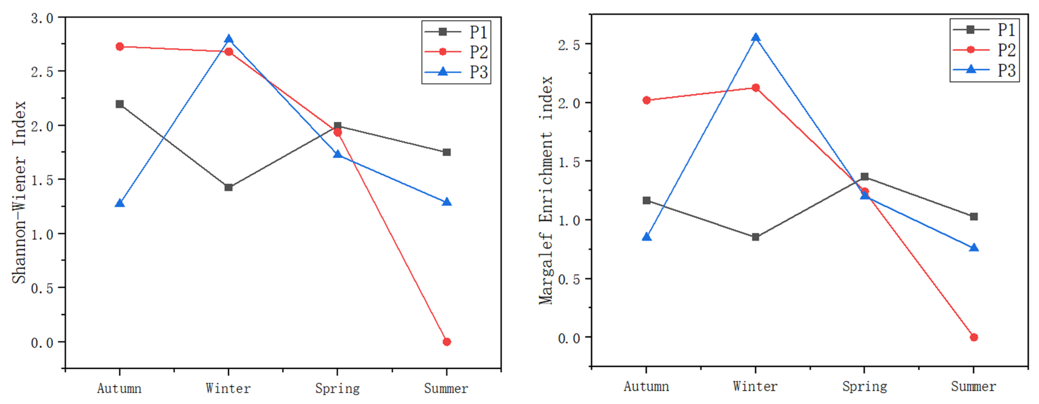
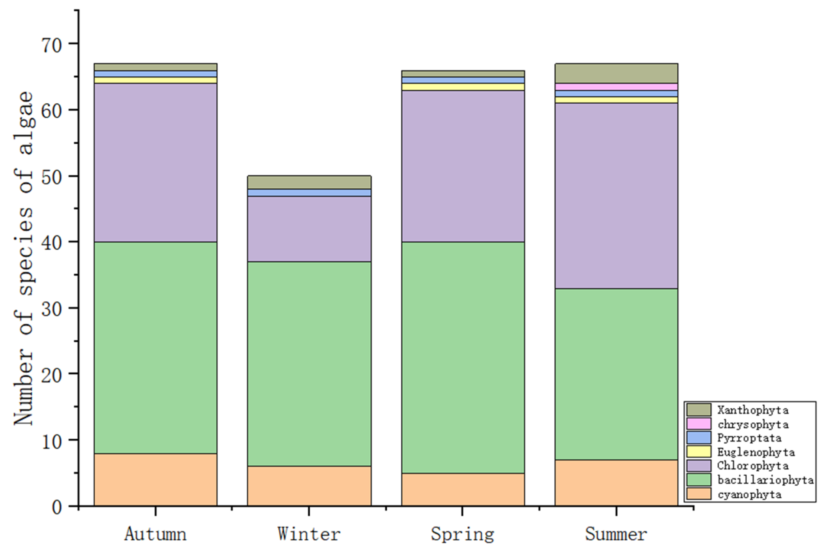
3.3.2. Algal Community Structure

During the experiment, 130 species of phytoplankton from seven phyla were collected in the study river, including 15 species of Cyanophyta, 54 species of diatoms, 51 species of Chlorophyta, four species of Xanthophyta, four species of Euphyta, one species of dinoflagellates, and one species of Chrysophyta. Diatoms and Chlorophyta were the main species in the Pi River, accounting for 41.54% and 39.23% of all the algal species, respectively. Cyanobacteria accounted for 11.54%, Xanthophyta and Euglenophyta accounted for 3.08%, and dinoflagellates and Chrysophyta accounted for 0.77%. From the perspective of temporal change, the number of algae species in winter was the lowest in the whole year, especially Chlorophyta, which had only 10 species in winter (24 species in autumn, 23 species in spring, and 28 species in summer), which significantly differed from the other seasons (Figure 7). The number of algae species at various points in the Pi River varied widely, ranging from 14 to 49 species, with the highest value appearing at the downstream point in autumn and the lowest value appearing in the middle point in summer. The number of algal species in P1 was stable during the test, while the number in P2 fluctuated greatly. The annual average value was significantly lower in P2 than in P1 and P3. The number of algal species in P3 were relatively low in winter and stable in other seasons, with an average value of 37 species.

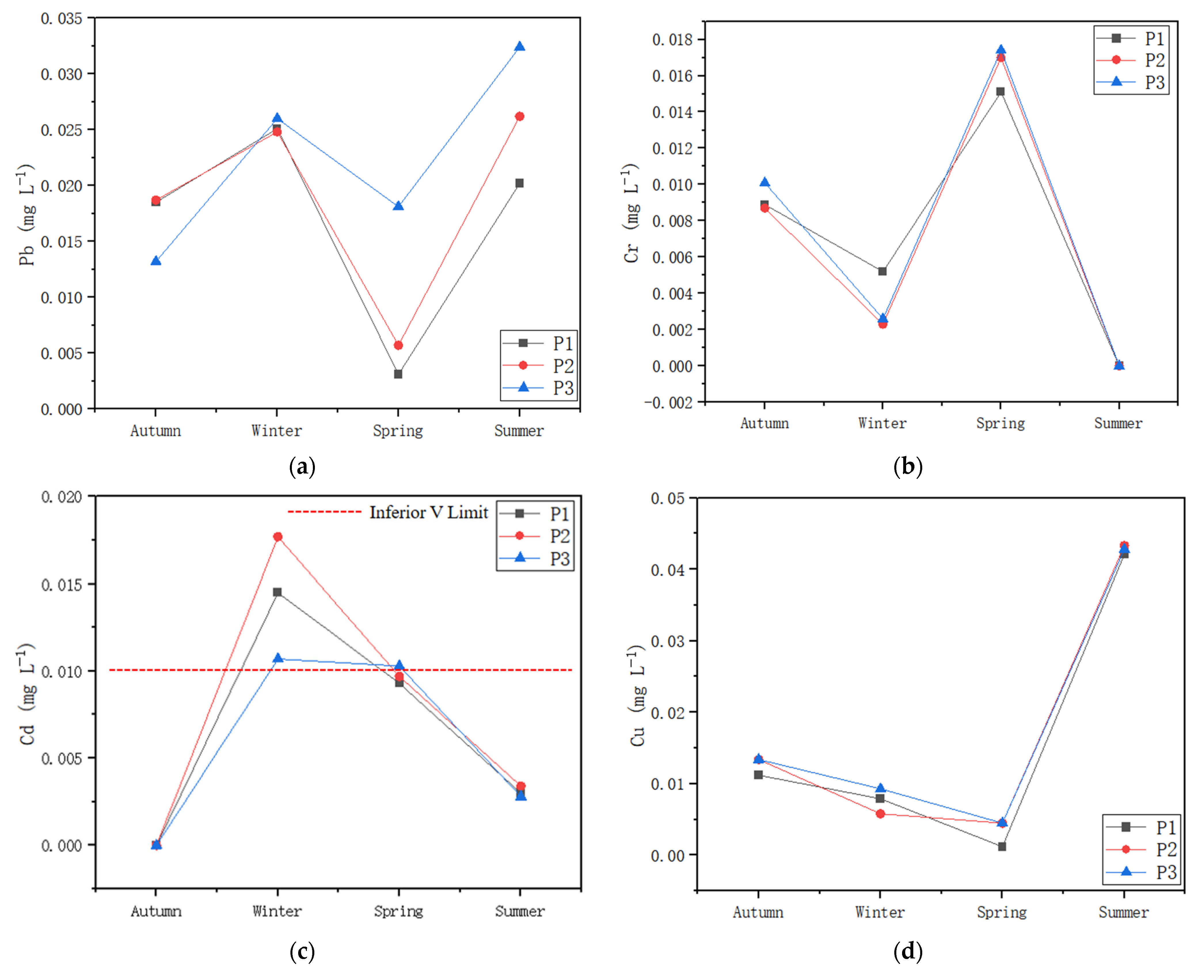
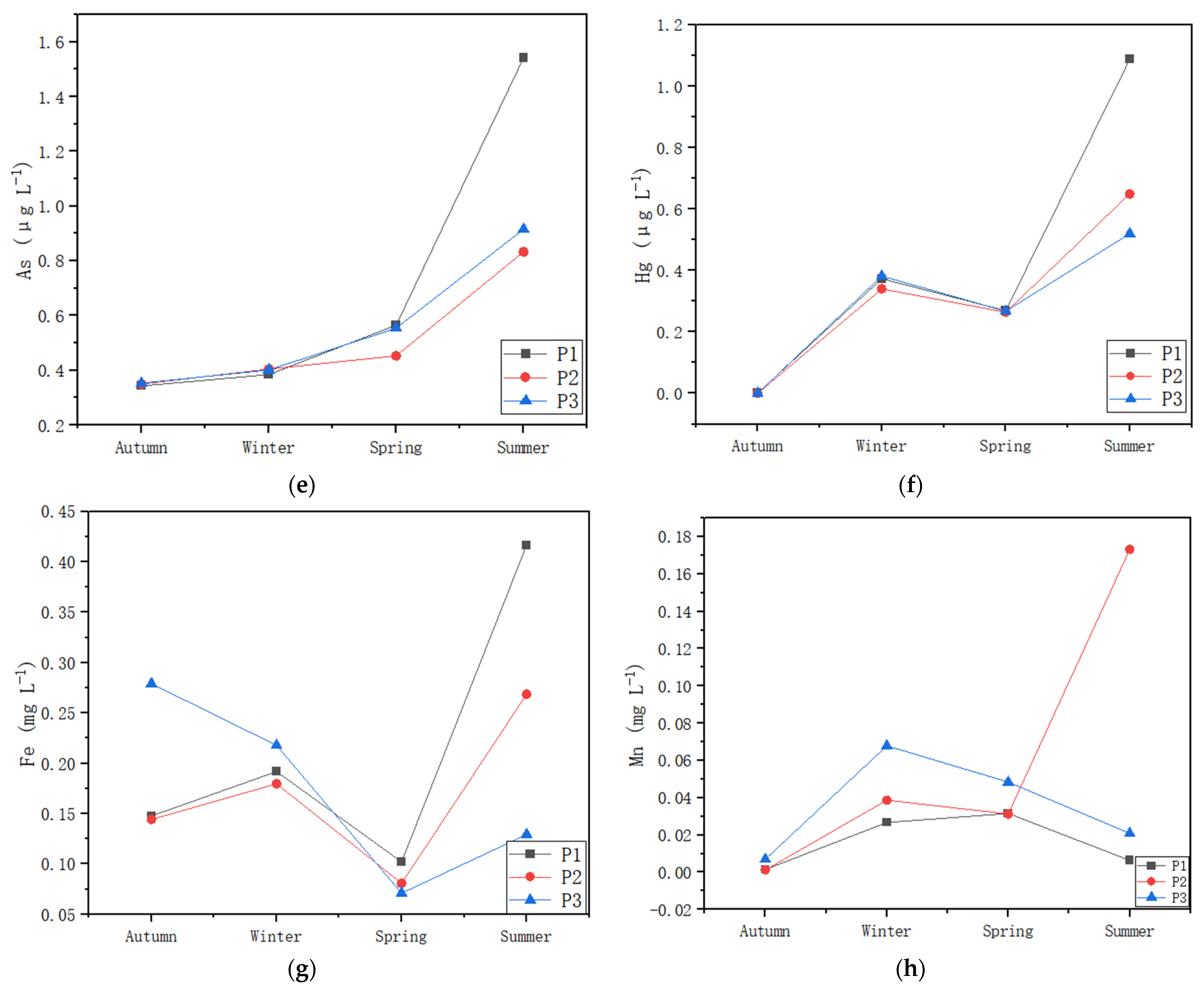
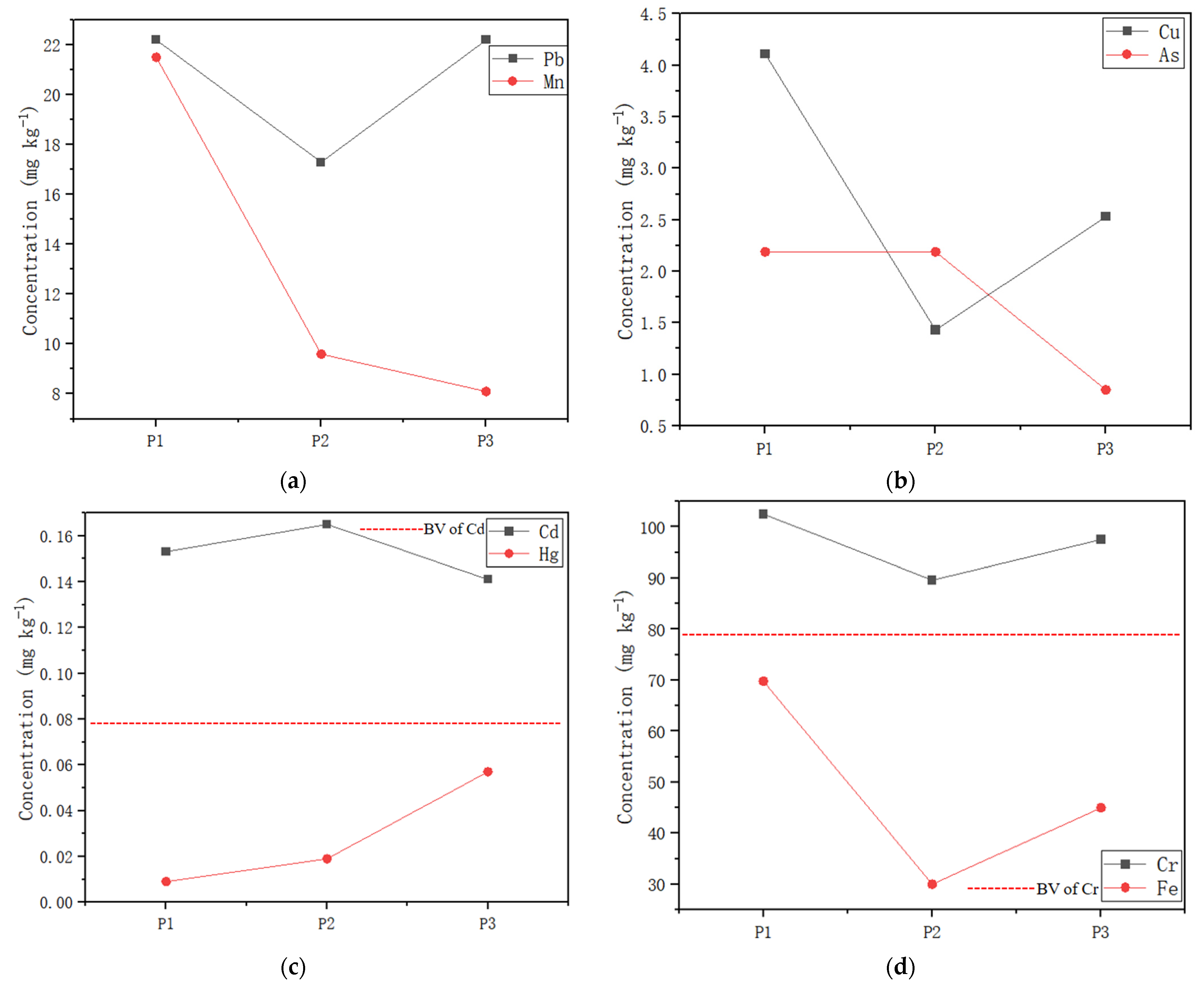
3.4. Metals in Water and Sediment

This study detected and analyzed eight kinds of metals in the water and sediment of the Pi River (Table 8; Table 9). Cd in the water exceeded the class V water limit, which indicated that the water body was seriously polluted by Cd (0.0165 mg L−1) in winter, and heavy metals in the water were relatively stable. The spatiotemporal variation in heavy metals in the water is shown in Figure 8.
The Spearman correlation analysis showed that the Pb content was significantly positively correlated with the Cd content (p < 0.05, r2 = 0.336 *). Hg was positively correlated with As and Fe (p < 0.01, r2 = 0.588 **; p < 0.01, r2 = 0.650 **), while As was positively correlated with Fe, and the correlation coefficient was (p < 0.01, r2 = 0.612 **). There was a significant positive correlation between Fe and Mn (p < 0.05, r2 = 0.353 *). The correlation analysis showed that metals with higher correlation coefficients may have been influenced by the same factors, and their sources or migration and transformation mechanisms might be similar.
Except for Cd and Cr, the metal contents in the other sediments did not exceed the background values of the heavy metal contents in the soil of Sichuan Province (BV) [27]. The contents of Cd and Cr at all the sampling sites exceeded the standard, and the contents of Cd were 0.153, 0.165, and 0.141 mg kg−1, which were 1.93, 2.08, and 1.78 times the background value, respectively. The Cr contents were 102.5, 89.6, and 97.5 mg kg−1, which were 1.29, 1.13, and 1.23 times the background value, respectively (Figure 9).
The PCA results (Table 10) showed that the first principal components of the Pi River were Pb, Hg, Cu, As, and Fe. Hg, As, and Fe were positively correlated with each other, and Mn and Fe were positively correlated. This phenomenon suggested that the heavy metals in the study river may have come from a similar source. The second principal component contained Cd and Mn.

4. Discussion

4.1. Water Environment Polluted by Nutrients

In this work, we found that the water of the studied river was polluted in February (WPI = 192.53), which was similar to the analysis of the water eutrophication status. The TLI was 59.1 in winter, which was higher than that in the mean flow period. The significant increase in the WPI in February indicated that the river could be seriously polluted during the investigation, owing to the impact of human activities on the river. Additionally, except in winter, the eutrophication status of the Pi River showed obvious spatial differences. The eutrophication degree was the lowest in the upper reaches (53.89), and the most serious eutrophication degree was in the lower reaches (62.75).
Moreover, the water quality indexes showed an obvious seasonality. For instance, the TP, TOC, COD, AN, and Chl-a all reached their peak values in winter but remained at relatively low levels in the mean flow period. The significant correlation of these indexes indicated that there may be homology. The source of nutrients may be the input of industrial sewage. The source input form resulted in unbalanced TN:TP. The N and P in the river varied greatly with different flowing areas, and their bioavailable forms also varied with different inputs [28]. The TN:TP ratios of the river in the other periods were all less than 10 units and were in an N restriction state, except for TN:TP > 10 in February, April, June, and July. Previous studies have shown that a water environment with low N and high P is the most suitable for Cyanophyta species growth [3,28]. For example, the optimal TN:TP growth ratio of Microcystis in Cyanophyta is 9:1 [29], and it might become the dominant species in still water. In spring/summer, Oscillatoria princeps and O. agardhii species were found at different sampling sites, indicating that the water in the Pi River in spring and summer was suitable for Cyanophyta algae growth. However, there were no signs of algal blooms observed at the sampling sites. It is now generally accepted that Chl-a represents a photoautotrophic phytoplankton signature in water. This value could not only be used to measure phytoplankton quantity but could also be an important indicator of productivity and the eutrophication level [30]. Our results showed that, although the nutrient conditions in the Pi River reached the conditions for cyanobacterial blooms, the blooms were restrained by other restrictive conditions. However, other studies have expressed uncertainty about the relationship between TN:TP and cyanobacterial species dominance in water. Studies have shown that TN:TP has no significant correlation with the dominance of cyanobacteria [31]. These studies concluded that the release of P from sediments was activated by the outbreak of cyanobacteria under sufficient nutrient conditions. Therefore, a low TN:TP ratio might be the result rather than the cause of cyanobacterial outbreaks [32].
The Chl-a of the studied river was higher in warmer times (spring and summer) than in cooler times. The flow rose sharply due to upstream inflow in spring and summer with increasing rain runoff. Additionally, turbidity increased and the suspended solids in the water and sediment were susceptible to disturbance, resulting in a decrease in the settling velocity of the suspended material in the river, which led to the deterioration of the water and light conditions. Algal biomass still had the potential to decline even if the other conditions for survival were met [33]. Previous studies have revealed that the rate of algal growth and reproduction is low in temperate rivers and that the occurrence of blooms is closely related to the water retention time and is obviously transient [34,35]. European studies have also documented short-lived algal blooms in the lower Rhine River basin during summer [36], but river blooms are more likely to occur in warmer tropical/subtropical regions. Some scholars have argued that slow river flow is an important cause of bloom formation, and that adequate upstream recharge and river flow is one of the most effective ways to curb blooms [37]. The nutrient elements in the Pi River were limited by N, making the river suitable for algae breeding. With the increase in water temperature in spring and summer, the slow flow rate in the middle and lower reaches enabled algal growth, which could have potentially caused an algal bloom. However, with the increase in temperature, the upcoming water from the upper reaches of the Pi River and the runoff of rainwater along the basin increased the total river flow. The sudden increase in the overall flow made most algae unfit for their original environment. For example, only 14 species of algae were documented in P2 in summer, which was the minimum value found in all the periods.
Studies have shown that plankton can accelerate the utilization of inorganic carbon under relatively stable hydraulic conditions after heavy rainfall or runoff [38]. Therefore, we speculated that the great difference in hydraulic conditions may be an important difference in the mechanism of eutrophication in different water bodies. Compared with still water, the water flow in urban rivers accelerates an increase in the DO content and improves the capacity of water to contain and buffer high contents of nutrients, which may also explain the suppression of aquatic eutrophication in the Pi River.

4.2. Aquatic Communities Affected by Heavy Metals in Water/Sediment

The PCA showed that the river was polluted by metals. Most of the businesses along the Pi River are industrial manufacturing, including electronics manufacturing, the building materials industry, and the transportation industry. The wastewater and dust brought by these industries may have entered the water body through rain leaching and atmospheric precipitation, making industry a main source of heavy metals [39]. The agricultural land surrounded by P3 was relatively scattered. The land is mismanaged, and there is often waste piled on both banks of the river. Metals can also be affected by microbes and rainwater leaching from the garbage leachate into the water, and garbage burning can cause pollutants that are deposited by atmospheric precipitation into water bodies. These reasons may explain why the river was polluted by heavy metal pollution. Therefore, the relevant departments and organizations of river protection should pay attention to the above situation.
In this study, the Shannon–Wiener (H’) and Margalef’s (dM) indexes of benthic macroinvertebrates in the Pi River were calculated. Then, a correlation analysis between them and the heavy metal content in sediments was carried out. As shown in Table 11, Cd was significantly negatively correlated with dM in the sediments. According to the literature, the interaction between the water flow and sediment nutrient content varies in wet and dry seasons. At different times, nutrients and metal-rich inputs from these sources may exceed the nutrient requirements for benthic communities and lead to ecosystem saturation or health hazards, a situation frequently documented and observed in urban rivers worldwide [40]. Macrobenthos in rivers are widely distributed, but their activities are limited, and their range is bound to their own habitat. Most benthic communities live in river sediments, and their community structure and diversity can effectively reveal the heavy metal concentration in rivers [41]. Although Oligochaeta pollution-resistant benthic species began to appear in the middle reaches of the Pi River, they were not dominant species, indicating that the water quality began to deteriorate by the middle reaches.
Many studies have shown that benthic animals are sensitive to heavy metals in water and sediment. In areas with high heavy metal contents, the species diversity of benthic macroinvertebrates is lower, and pollution-tolerant species are normally the dominant species. Therefore, many scholars regard benthic animals as indicator species that can be used to evaluate river pollution [42]. The abundance of major gastropods, such as Chironomus, was significantly positively correlated with metal concentrations in sediments, and thus could be used as indicators of heavy metal pollution [43]. Tendipus spp. were the dominant benthic species in the lower reaches of the Pi River in winter and spring. The Cd content in the water peaked at all the sampling points in winter. These phenomena indicated that the water quality downstream was seriously polluted by Cd, and the benthic community had completely changed compared to the community of the upstream reaches that had cleaner water. However, the H’ and dM indexes showed that the P3 index in winter was higher than that in the other seasons. We speculated that this difference might have been due to the influence of the emergence of many pollution-resistant species. Therefore, we believe that these two indexes alone cannot comprehensively and objectively represent the river water quality.
Cd is one of the most polluted heavy metal elements in water bodies in Southwest China. Cd is easily absorbed by and stored in organisms with lasting toxicity and has a great impact on the growth of algae [44]. There was a significant negative correlation between Cd and Chl-a (r2 = −0.330 *, p < 0.05), indicating that Cd had a serious impact on algal reproduction in the river. Aquatic organisms have a strong ability to enrich Cd at levels up to a thousand times higher than those in water bodies [45]. Moreover, metals are not always in a stable state in sediments, and Cd in sediments will be redissolved in water after the disturbance of aquatic habitats [46]. Previous research has shown that the acid soluble state is the most sensitive to the heavy metal form under the action of a disturbing force, and a high intensity disturbance can promote the oxidation of the oxidizable heavy metal state. The disturbance will decompose the large particles into small particles, and the heavy metals will be released again after the resuspension process [47,48]. Cd inhibits chlorophyll synthesis and affects photosynthesis by combining with the thylakoid membrane of algal cells [49]. It has been found that the contents of chlorophyll a and b in Chlorella vulgaris under Cd stress gradually decrease [50]. Other scholars conducted physiological response tests on Tetradesmus obliquus under Cd stress at different concentrations, and the results showed that the chlorophyll concentration of algal cells decreased under Cd stress at high concentrations [51]. Cd not only affects the chlorophyll concentrations of algae but also obviously harms its antioxidant system. When the concentration of Cd in water increased, the contents of hydrogen peroxide and superoxide anion in algae increased, leading to a significant increase in the MDA levels in algae. Other cellular substances of algae, such as proteins and soluble sugars, decrease with increasing Cd concentrations [52].

5. Conclusions

This research revealed that the Pi River, as the alternate underground water source for Chengdu, was heavily polluted for most of the year, with February being the most polluted and eutrophication being the most serious in the downstream reaches, according to the value that exceeded the limit in China. It is speculated that the failure of algal blooms in the Pi River was due to the influence of hydrodynamic conditions. In addition, we found that the water of the Pi River was seriously polluted by heavy metals, which may be caused by the industrial distribution in the Pi River basin. According to our study on the influence of heavy metals and aquatic animal communities in sediments, the Cd in the sediments of the Pi River had a serious impact on benthic reproduction and had a significant negative effect on algal reproduction. Cd in the sediment far exceeded the soil background value of Sichuan Province and was easily disturbed by the environment, leading to secondary pollution. Based on the above results, we suggest that relevant river protection departments and social organizations strengthen monitoring approaches for the quality of the Pi River and strictly control the discharge of industrial sewage and agricultural nonpoint source pollution.

Author Contributions

D.L.: Conceptualization, methodology, software, formal analysis, investigation, data curation, writing—original draft. L.L.: Writing—review and editing. Q.D.: Investigation. R.W.: Software, data curation. T.X.: Writing—review and editing. L.Q.: Writing—review and editing, funding acquisition. Z.W.: Writing—review and editing. B.L.: Formal analysis, investigation, data curation. S.L.: Conceptualization, methodology, data curation, writing—review and editing, funding acquisition. Q.C.: Conceptualization, supervision, project administration, funding acquisition. All authors have read and agreed to the published version of the manuscript.

Funding

This work was partially supported by the General Fund Project of the Natural Sciences Foundation of Hubei Province (Grant No. 2022CFB334), the State Key Laboratory of Tropical Oceanography, the South China Sea Institute of Oceanology, the Chinese Academy of Sciences (Grant No. LTO2219), the Scientific Research Project of the Geophysical Exploration Brigade of Hubei Provincial Bureau of Geology (Project No. WTDKJ2022-3), the Leadership Talent Program of the Tianfu Emei Plan in Sichuan Province (No. CHUANEMEI2105), and the Funding for Doctoral Training at Sichuan Agricultural University, China.

Data Availability Statement

Not applicable.

Acknowledgments

The authors are thankful to all the testing companies/institutions and assistants for their help in designing/conducting the experiments, analyzing the data, and writing/revising the manuscript.

Conflicts of Interest

The authors declare no conflict of interest.

References

  1. Carpenter, S.R.; Christensen, D.L.; Cole, J.J.; Cottingham, K.L.; He, X.; Hodgson, J.R.; Kitchell, J.F.; Knight, S.E.; Pace, M.L. Biological control of eutrophication in lakes. Environ. Sci. Technol. 1995, 29, 784–786. [Google Scholar] [CrossRef]
  2. Smith, V.H.; Joye, S.B.; Howarth, R.W. Eutrophication of Freshwater and Marine Ecosystems. Limnol. Oceanogr. 2006, 51, 351. [Google Scholar] [CrossRef]
  3. Monteagudo, L.; Moreno, J.L.; Picazo, F. River eutrophication: Irrigated vs non-irrigated agriculture through different spatial scales. Water Res. 2012, 46, 2759–2771. [Google Scholar] [CrossRef] [PubMed]
  4. Sala, O.E.; Chapin, F.S.; Armesto, J.J.; Berlow, E.; Bloomfield, J.; Dirzo, R.; Huber-Sanwald, E.; Huenneke, L.F.; Jackson, R.B.; Kinzig, A.; et al. Global biodiversity scenarios for the year 2100. Science 2000, 287, 1770–1774. [Google Scholar] [CrossRef] [PubMed]
  5. Lee, C.W.; Kwon, H.B.; Jeon, H.P.; Koopman, B. A new recycling material for removing phosphorus from water. J. Clean. Prod. 2009, 17, 683–687. [Google Scholar] [CrossRef]
  6. Camargo, J.A.; Alonso, A. Ecological and toxicological effects of inorganic nitrogen pollution in aquatic ecosystems: A global assessment. Environ. Int. 2006, 32, 831–849. [Google Scholar] [CrossRef] [PubMed]
  7. Lynam, C.P.; Cusack, C.; Stokes, D. A methodology for community-level hypothesis testing applied to detect trends in phytoplankton and fish communities in Irish waters. Estuar. Coast. Shelf Sci. 2010, 87, 451–462. [Google Scholar] [CrossRef]
  8. Rizzo, L.; Manaia, C.; Merlin, C.; Schwartz, T.; Dagot, C.; Ploy, M.C.; Michael, I.; Fatta Kassinos, D. Urban wastewater treatment plants as hotspots for antibiotic resistant bacteria and genes spread into the environment: A review. Sci. Total Environ. 2013, 447, 345–360. [Google Scholar] [CrossRef] [PubMed]
  9. Tylmann, W. Lithological and geochemical record of anthropogenic changes in recent sediments of a small and shallow lake (Lake Pusty Staw, northern Poland). J. Paleolimnol. 2005, 33, 313–325. [Google Scholar] [CrossRef]
  10. Jahan, Z.; Hajira, T.; Othman, A.; Habeebullah, T.M.; Sayqal, A.; Assaggaf, H.M.; Ahmed, O.B.; Sultan, M.; Mohiuddin, S.; Masood, S.S.; et al. Geo-environmental approach to assess heavy metals around auto-body refinishing shops using bio-monitors. Heliyon 2022, 8, e08809. [Google Scholar]
  11. Liu, X.; Jiang, Y.; Gao, J.F.; Yin, H.B.; Cai, Y.J. Heavy metal pollution characteristics and risk assessment of Chaohu Lake District and main access rivers. J. Lake Sci. 2016, 28, 502–512. [Google Scholar]
  12. Chen, R.; Ao, D.; Ji, J.; Wang, X.C.; Li, Y.Y.; Huang, Y.; Xue, T.; Guo, H.; Wang, N.; Zhang, L. Insight into the risk of replenishing urban landscape ponds with reclaimed wastewater. J. Hazard. Mater. 2017, 324, 573–582. [Google Scholar] [CrossRef] [PubMed]
  13. Anon. Impacts of land use and water quality on macroinvertebrate communities in the Pearl River drainage basin, China. Hydrobiologia 2010, 652, 71–88. [Google Scholar] [CrossRef]
  14. Wang, Y.; Li, B.L.; Feng, Q.; Wang, Z.; Liu, W.; Zhang, X.; Kong, D.; Zuo, Y. Space distribution of heavy metals and its relationship with macrozoobenthos in the Heihe River, northwest China. China Environ. Sci. 2021, 41, 1354–1365. [Google Scholar]
  15. Costas, N.; Pardo, I.; Méndez-Fernández, L.; Martínez-Madrid, M.; Rodríguez, P. Sensitivity of macroinvertebrate indicator taxa to metal gradients in mining areas in Northern Spain. Ecol. Indic. 2018, 93, 207–218. [Google Scholar] [CrossRef]
  16. Bere, T.; Dalu, T.; Mwedzi, T. Detecting the impact of heavy metal contaminated sediment on benthic macroinvertebrate communities in tropical streams. Sci. Total Environ. 2016, 572, 147–156. [Google Scholar] [CrossRef] [PubMed]
  17. Paithankar, J.G.; Saini, S.; Dwivedi, S.; Sharma, A.; Chowdhuri, D.K. Heavy metal associated health hazards: An interplay of oxidative stress and signal transduction. Chemosphere 2021, 262, 128350. [Google Scholar] [CrossRef] [PubMed]
  18. Baudou, F.G.; Ossana, N.A.; Castañé, P.M.; Mastrángelo, M.M.; Ferrari, L. Cadmium effects on some energy metabolism variables in Cnesterodon decemmaculatus adults. Ecotoxicology 2017, 26, 1250–1258. [Google Scholar] [CrossRef] [PubMed]
  19. Liu, C.L. Aquatic Environmental Diagnosis and Water Quality Target Management Suggestion for the Tuojiang Basin (Chengdu Section). Ecol. Environ. Monit. Three Gorges 2022, 7, 34–41. [Google Scholar]
  20. The Ministry of Ecology and Environment of the People’s Republic of China (MEEC). Standard Methods for the Examination of Water and Wastewater, 4th ed.; Chinese Environmental Science Press: Beijing, China, 2002.
  21. Jahan, Z.; Mohammad, W.; Shah, S.A.; Khanam, S.; Tahir, H.; Qadri, M. Characterization of sand samples from Karachi beaches using gamma Spectrometry and xrd. Radiat. Prot. Dosim. 2020, 189, 234–241. [Google Scholar]
  22. ISO/TC147/SC2–PHYSICAL; Chemical and Biochemical Methods. CP 401-1214. Vernier: Geneva, Switzerland, 1971.
  23. Environmental Quality Standards for Surface Water, National Standard of the People’s Republic of China; Ministry of Ecology and Environment, People’s Republic of China: Beijing, China, 2002.
  24. Brankov, J.; Milijašević, D.; Milanović, A. The Assessment of the Surface Water Quality Using the Water Pollution Index: A Case Study of the Timok River (The Danube River Basin), Serbia. Arch. Environ. Prot. 2012, 38, 49–61. [Google Scholar] [CrossRef]
  25. Ren, R.; Jun, H. An introduction of endocrine disrupters (EDCs). Safety Environ. Eng. 2004, 11, 7–10. [Google Scholar]
  26. Aizaki, M.; Otsuki, A.; Fukushima, T.; Kawai, T.; Hosomi, M.; Muraoka, K. Application of modified Carlson’s trophic state index to Japanese lakes and its relationships to other parameters related to trophic state. Res. Rep. Natl. Inst. Environ. Stud. 1981, 23, 13–31. [Google Scholar]
  27. Zhang, H.Z.; Tang, Y.L.; Lu, J.; Zhou, H.; Xu, Y.Q.; Chen, C.; Zhao, Y.; Wang, M.E. Sources and spatial distribution of typical heavy metal pollutants in soils in Xihu scenic area. Environ. Sci. 2014, 35, 1516–1522. [Google Scholar]
  28. Neal, C.; Hilton, J.; Wade, A.J.; Neal, M.; Wickham, H. Chlorophyll-a in the rivers of eastern England. Sci. Total Environ. 2006, 365, 84–104. [Google Scholar] [CrossRef] [PubMed]
  29. Kilham, S.S.; Kilham, P. The importance of resource supply rates in determining phytoplankton community structure. Am. Assoc. Adv. Sci. Symp. 1984, 85, 7–27. [Google Scholar]
  30. Deng, T.A.; Chau, K.W.; Duan, H.F. Machine learning based marine water quality prediction for coastal hydro-environment management. J. Environ. Manag. 2021, 284, 112051. [Google Scholar] [CrossRef] [PubMed]
  31. Wu, N.; Schmalz, B.; Fohrer, N. Distribution of phytoplankton in a German lowland river in relation to environmental factors. J. Plankton Res. 2011, 33, 807–820. [Google Scholar] [CrossRef]
  32. Xie, L.Q.; Xie, P.; Li, S.X.; Tang, H.; Liu, H. The low TN: TP ratio, a cause or a result of Microcystis blooms? Water Res. 2003, 37, 2073–2080. [Google Scholar] [CrossRef] [PubMed]
  33. Köhler, J.; Bahnwart, M.; Ockenfeld, K. Growth and Loss Processes of Riverine Phytoplankton in Relation to Water Depth. Int. Rev. Hydrobiol. 2002, 87, 241–254. [Google Scholar] [CrossRef]
  34. Krogmann, D.W.; Butalla, R.; Sprinkle, J. Blooms of Cyanobacteria on the Potomac River. Plant Physiol. 1986, 80, 667–671. [Google Scholar] [CrossRef] [PubMed]
  35. Reinhard, E.G. The plankton ecology of the upper Mississippi, Minneapolis to Winona. Ecol. Monogr. 1931, 1, 396–464. [Google Scholar] [CrossRef]
  36. Ibelings, B.; Admiraal, W.; Bijkerk, R.; Ietswaart, T.; Prins, H. Monitoring of algae in Dutch rivers: Does it meet its goals? J. Appl. Phycol. 1998, 10, 171–181. [Google Scholar] [CrossRef]
  37. Bormans, M.; Maier, H.; Burch, M.; Baker, P. Temperature stratification in the lower River Murray, Australia: Implication for cyanobacterial bloom development. Mar. Freshw. Res. 1997, 48, 647–654. [Google Scholar] [CrossRef]
  38. Cózar, A.; Echevarría, F. Size structure of the planktonic community in microcosms with different levels of turbulence. Sci. Mar. 2005, 69, 187–197. [Google Scholar] [CrossRef]
  39. Jiao, W.; Lu, S.Y.; Li, G.D. Heavy metal pollution and ecological risk assessment around Taihu Lake. J. Appl. Environ. Biol. 2010, 16, 577–580. [Google Scholar]
  40. Weigelhofer, G. The potential of agricultural headwater streams to retain soluble reactive phosphorus. Hydrobiologia 2017, 793, 149–160. [Google Scholar] [CrossRef]
  41. Armitage, P.; Moss, D.; Wright, J.; Furse, M. The performance of a new biological quality score system based on macroinvertebrate over a wide range of unpolluted running waters. Water Res. 1983, 17, 333–347. [Google Scholar] [CrossRef]
  42. Rasmussen, J.J.; McKnight, U.S.; Loinaz, M.C.; Thomsen, N.I.; Olsson, M.E.; Bjerg, P.L.; Binning, P.J.; Kronvang, B. A catchment scale evaluation of multiple stressor effects in headwater streams. Sci. Total Environ. 2013, 442, 420–431. [Google Scholar] [CrossRef] [PubMed]
  43. Wang, X.X.; Su, P.; Lin, Q.D.; Song, J.X.; Sun, H.T.; Cheng, D.D.; Wang, S.Q.; Peng, J.L.; Fu, J.X. Distribution, assessment and coupling relationship of heavy metals and macroinvertebrates in sediments of the Weihe River Basin. Sustain. Cities Soc. 2019, 50, 101665. [Google Scholar] [CrossRef]
  44. Li, Q.Q.; Zhang, S.Y.; Dai, T.F.; Gao, X.S.; Zhang, X.; Wang, C.Q.; Yuan, D.G.; Li, K.R. Contents and Sources of Cadmium in Farmland Soils of Chengdu Plain, China. J. Agro-Environ. Sci. 2014, 33, 898–906. [Google Scholar]
  45. Huang, X.H.; Zhou, Y.M.; Wang, Y.H.; Ma, Y.G.; Dai, Y.J. Effects of LA-GLy-VB6 on plants under PB-Cd combined stress. Urban Environ. Urban Ecol. 2001, 14, 1–3. [Google Scholar]
  46. Beutel, M.W.; Leonard, T.M.; Dent, S.R.; Moore, B.C. Effects of aerobic and anaerobic conditions on P, N, Fe, Mn and Hg accumulation in waters overlaying profundal sediments of anoligo-mesotrophic lake. Water Res. 2008, 42, 1953–1962. [Google Scholar] [CrossRef] [PubMed]
  47. Krishnankutty, N.; Idris, M.; Hamzah, F.M.; Manan, Y. The chemical form and spatial variation of metals from sediment of Jemberau mining region of Tasik Chini, Malaysia. Environ. Sci. Pollut. Res. 2019, 26, 25046–25056. [Google Scholar] [CrossRef] [PubMed]
  48. Liu, X.Z.; Liu, Q.Q.; Wang, W.J.; Sheng, Y.Q. Effects of hydraulic perturbation on rerelease of heavy metals from estuarine sediments. J. Ecol. Rural. Environ. 2020, 36, 1460–1467. [Google Scholar]
  49. Devoy, J.; Géhin, A.; Müller, S.; Melczer, M.; Remy, A.; Antoine, G.; Sponne, I. Evaluation of chromium in red blood cells as an indicator of exposure to hexavalent chromium: An in vitro study. Toxicol. Lett. 2016, 255, 63–70. [Google Scholar] [CrossRef] [PubMed]
  50. Huang, Z.Y.; Li, L.P.; Huang, G.L. Growth-inhibitory and metal-binding proteins in Chlorella vulgaris exposed to cadmium or zinc. Aquat. Toxicol. 2009, 91, 54–61. [Google Scholar] [CrossRef] [PubMed]
  51. Duan, C.X.; Zhang, B.Y.; Wu, S.C.; Feng, J.; Wang, G. Effects of Heavy Metal Cadmium on photosynthesis of Heterophyllum heterophyllum. Oceanol. Limnol. Sin. 2015, 46, 351–356. [Google Scholar]
  52. Piovar, J.; Stavrou, E.; Kaduková, J.; Kimáková, T.; Bačkor, M. Influence of long-term exposure to copper on the lichen hotobiont Trebouxia erici and the free-living algae Scenedesmus quadricauda. Plant Growth Regul. 2011, 63, 81–88. [Google Scholar] [CrossRef]
Figure 1. The temperature and rainfall ranges in Chengdu from 2021 to 2022. The data in the above figure was obtained from the public data of the Chengdu Meteorological Bureau.
Water 15 03640 g001
Figure 2. Sampling sites along the Pi River. The image provided above is an adapted representation created using Baidu® Maps (https://map.baidu.com/; accessed on 10 May 2022) for reference.
Water 15 03640 g002
Figure 3. Variations in the water quality indicators in the Pi River: (a) concentrations of the TN and TP; (b) concentrations of DO and the TOC; (c) concentrations of Chl-a and the BOD5; (d) EC and AN; (e) the COD and T; (f) turbidity and the SD.
Water 15 03640 g003
Figure 4. The monthly WPI values of the Pi River. CI: confidence interval.
Water 15 03640 g004
Figure 5. The seasonal TLI (∑) indexes for September 2020 to August 2021 for the Pi River.
Water 15 03640 g005
Figure 6. The spatiotemporal variations of the Shannon–Wiener index (H’; left) and Margalef’s Richness Index (dM; right) in the Pi River.
Water 15 03640 g006
Figure 7. Community structure of algal species in the Pi River in different seasons.
Water 15 03640 g007
Figure 8. Changes in the heavy metal contents in water. (a) Contents of Pb; (b) contents of Cr; (c) contents of Cd; (d) contents of Cu; (e) contents of As; (f) concentrations of Hg; (g) contents of Fe; and (h) contents of Mn.
Water 15 03640 g008aWater 15 03640 g008b
Figure 9. Changes in the heavy metal contents in sediment: (a) contents of Pb and Mn; (b) contents of Cu and As; (c) contents of Cd and Hg; and (d) contents of Cr and Fe.
Water 15 03640 g009
Table 1. Classification of water quality and the corresponding WPI range.
Water Quality
Categories
IIIIIIIVVWorse than V
WPI value≤2020 < WPI ≤ 4040 < WPI ≤ 6060 < WPI ≤ 8080 < WPI ≤ 100>100
Table 2. Evaluation of the trophic level index.
Evaluation LevelQualitative Evaluation
TLI (∑) < 30OligotrophicVery clean
30 ≤ TLI (∑) < 50MesotrophicClean
50 < TLI (∑)EutrophicTypical
50 < TLI (∑) ≤ 60Lightly eutrophicLightly polluted
60 < TLI (∑) ≤ 70Moderately eutrophicModerately polluted
TLI (∑) > 70Severely eutrophicSeverely polluted
Table 3. The pollution classification of the Shannon—Wiener index calculated using Equation (7).
HH= 0H’ = 0–1H’ = 1–2H’ = 2–3H’ > 3
Pollution levelNo benthic communities were found; severe contaminationHeavy pollutionModerately pollutedMild pollutionNo pollution
Table 4. The pollution classification of Margalef’s index calculated using Equation (8).
dMdM < 1dM = 1–2dM = 2–3dM > 3
Pollution levelHeavy pollutionModerately pollutedMild pollutionNo pollution
Table 5. Variations in the water quality indicators.
ParametersRangeMean ± Std
pH7.24–8.257.78 ± 0.22
T (°C)6.30–26.1016.50 ± 5.21
SD (cm)4.00–122.0062.29 ± 26.78
Turbidity (FTU)6.20–205.0042.97 ± 46.70
EC (S m−1)289.00–691.00453.97 ± 107.74
DO (mg L−1)2.13–12.968.65 ± 2.55
TN (mg L−1)0.28–3.061.43 ± 0.80
TP (mg L−1)0.07–0.470.23 ± 0.12
AN (mg L−1)0.15–1.350.69 ± 0.30
COD (mg L−1)6.00–34.0021.22 ± 7.76
BOD5 (mg L−1)0.60–2.801.59 ± 0.56
Chl-a (mg L−1)0.041–11.572.47 ± 2.30
TOC (mg L−1)23.62–44.2532.21 ± 5.41
Table 6. Information on benthic invertebrates in the Pi River.
PhylaBenthonic Invertebrates
MolluskaCipangopaludina chinensis, Lymnaeidae, Viviparidae, Kimnoperna lacustris, Radix auricularia, R. suinhoi, Corbicula fluminea,
ArthropodaGammarus sp., Ecdyrus sp., Philopotamidae, and Cleantis sp. Macrobranchium nipponense, Caridina denticulata, Rhyacophilidae, Tendipus sp., Baetis sp., Caenis sp., and Aeshnidae
AnnelidaHiurdo sp., Limnodrilus sp., Hemiclepsis sp., and Glossiphonia sp.
PlatyhelminthesPlanaria sp.
Table 7. Temporal and spatial variations of the dominant benthic species in the Pi River.
PeriodP1P2P3
AutumnPhilopotamidae,
Gammarus sp.
Caridina denticulata, Philopotamidae,
Gammarus sp.,
Macrobranchium nipponense
WinterGammarus sp.Philopotamidae,
Gammarus sp.,
Rhyacophilidae,
Macrobranchium nipponense,
Tendipus sp.
SpringGammarus sp.Gammarus sp.Tendipus sp.
SummerGammarus sp.-Macrobranchium nipponense
Table 8. Summary of heavy metal contents detected in the water of the Pi River.
ParametersRangeStd ± Mean
Pb (mg L−1)0–0.0560.019 ± 0.021
Cr (mg L−1)0–0.0460.007 ± 0.014
Cd (mg L−1)0–0.0420.007 ± 0.010
Hg (μg L−1)0–2.5530.346 ± 0.499
As (μg L−1)0–3.7290.591 ± 0.760
Fe (mg L−1)0.009–1.0230.186 ± 0.195
Mn (mg L−1)0–0.4880.038 ± 0.082
Cu (mg L−1)0–0.0870.017 ± 0.026
Table 9. Description of the heavy metal concentrations in sediment, according to the national standards of China.
ParametersRangeStd ± Mean
Pb (mg L−1)17.00–22.2020.57 ± 2.83
Cr (mg L−1)89.60–102.5089.60 ± 102.50
Cd (mg L−1)0.14 –0.170.15 ± 0.01
Hg (μg L−1)0.01–0.050.03 ± 0.03
As (μg L−1)0.85–2.191.74 ± 0.77
Fe (mg L−1)30.00–69.8048.27 ± 20.10
Mn (mg L−1)8.10–21.5013.07 ± 7.34
Cu (mg L−1)1.43–4.112.69 ± 1.35
Table 10. Component matrix of the Pi River.
Component 1Component 2Component 3
Pb0.6350.461−0.524
Cr−0.854−0.2520.320
Cd−0.2500.7920.449
Hg0.8500.0950.498
As0.825−0.2900.422
Fe0.765−0.2280.073
Mn0.3560.5670.055
Cu0.920−0.193−0.140
Note: The bold numbers indicate higher loads.
Table 11. Correlation analysis of the metal elements and the Shannon—Wiener and Margalef’s indexes.
PbCrCdHgAsFeMnCu
H−0.667−0.086−0.2710.348−0.029−0.657−0.029−0.714
dM−0.691−0.0580.812 *0.441−0.265−0.667−0.029−0.638
Note: * indicates significant correlation.
Disclaimer/Publisher’s Note: The statements, opinions and data contained in all publications are solely those of the individual author(s) and contributor(s) and not of MDPI and/or the editor(s). MDPI and/or the editor(s) disclaim responsibility for any injury to people or property resulting from any ideas, methods, instructions or products referred to in the content.

