Article

Improving Forecasting Accuracy of Multi-Scale Groundwater Level Fluctuations Using a Heterogeneous Ensemble of Machine Learning Algorithms

by
Dilip Kumar Roy
1,*,
Tasnia Hossain Munmun
1,
Chitra Rani Paul
1,
Mohamed Panjarul Haque
1,
Nadhir Al-Ansari
2,* and
Mohamed A. Mattar
3
1
Irrigation and Water Management Division, Bangladesh Agricultural Research Institute, Gazipur 1701, Bangladesh
2
Department of Civil, Environmental and Natural Resources Engineering, Lulea University of Technology, 97187 Lulea, Sweden
3
Department of Agricultural Engineering, College of Food and Agriculture Sciences, King Saud University, P.O. Box 2460, Riyadh 11451, Saudi Arabia
*
Authors to whom correspondence should be addressed.
Water 2023, 15(20), 3624; https://doi.org/10.3390/w15203624
Submission received: 18 September 2023 / Revised: 12 October 2023 / Accepted: 13 October 2023 / Published: 16 October 2023

Abstract

:
Accurate groundwater level (GWL) forecasts are crucial for the efficient utilization, strategic long-term planning, and sustainable management of finite groundwater resources. These resources have a substantial impact on decisions related to irrigation planning, crop selection, and water supply. This study evaluates data-driven models using different machine learning algorithms to forecast GWL fluctuations for one, two, and three weeks ahead in Bangladesh’s Godagari upazila. To address the accuracy limitations inherent in individual forecasting models, a Bayesian model averaging (BMA)-based heterogeneous ensemble of forecasting models was proposed. The dataset encompasses 1807 weekly GWL readings (February 1984 to September 2018) from four wells, divided into training (70%), validation (15%), and testing (15%) subsets. Both standalone models and ensembles employed a Minimum Redundancy Maximum Relevance (MRMR) algorithm to select the most influential lag times among candidate GWL lags up to 15 weeks. Statistical metrics and visual aids were used to evaluate the standalone and ensemble GWL forecasts. The results consistently favor the heterogeneous BMA ensemble, excelling over standalone models for multi-step ahead forecasts across time horizons. For instance, at GT8134017, the BMA approach yielded values like R (0.93), NRMSE (0.09), MAE (0.50 m), IOA (0.96), NS (0.87), and a-20 index (0.94) for one-week-ahead forecasts. Despite a slight decline in performance with an increasing forecast horizon, evaluation indices confirmed the superior BMA ensemble performance. This ensemble also outperformed standalone models for other observation wells. Thus, the BMA-based heterogeneous ensemble emerges as a promising strategy to bolster multi-step ahead GWL forecasts within this area and beyond.

1. Introduction

Groundwater is a crucial resource of water for fulfilling the requirements of different sectors, such as domestic, industrial, and agricultural sectors. Unfortunately, the unsustainable extraction of groundwater resources has caused a reduction in the availability of this resource, leading to a notable disparity between the amount of groundwater available and the amount that is required to fulfill the needs. The unsustainable withdrawal of groundwater for irrigation practices is causing the annual extraction of groundwater beyond its natural replenishment capacity. This highlights the urgent requirement for the implementation of sustainable measures to manage groundwater resources. Changes in climate, such as alterations in precipitation patterns and temperature, can influence the rate at which groundwater is replenished, resulting in a decline in groundwater levels (GWL) in aquifers. Moreover, human activities, including land use modifications like deforestation and urbanization, can decrease the amount of water recharge rates in the groundwater aquifers. In Bangladesh, groundwater is a major source of drinking water and it plays a significant role in the agricultural sector. However, the overexploitation of groundwater through excessive pumping for irrigation purposes has resulted in declining GWLs in multiple regions, causing water scarcity and deteriorating water quality [1]. According to a recent study, the rate of groundwater depletion in Bangladesh has escalated from 1980 to 2019, leading to a significant impact on agricultural productivity and water availability [2]. To address these issues, forecasting the accuracy of GWL is essential for managing water resources effectively and minimizing the effects of climate change on water availability.
The use of Machine Learning (ML) algorithms in GWL forecasting has become more frequent as they are capable of processing large amounts of data and capturing nonlinear relationships between predictors and response variables. On the other hand, obtaining comprehensive knowledge about aquifer processes, geometry, and modeling techniques required for physically based numerical simulation models can be challenging due to data limitations, especially in developing countries like Bangladesh. Therefore, these models usually rely on assumptions and simplifications. Physically based numerical simulation models can be affected by significant uncertainties and errors in areas with limited monitoring data, mainly due to data scarcity and poor quality [3]. Additionally, physically based models may encounter inaccuracies in their predictions due to simplifications and assumptions made during the modeling process, leading to structural errors [4]. These limitations have prompted researchers to seek alternative modeling approaches, such as data-driven modeling, that can overcome these issues.
On the other hand, ML-based models are commonly considered to be a “black box” model because they use algorithms to analyze and identify patterns in data without the need for explicit programming instructions. Nevertheless, the nonlinear dynamics of aquifer responses can be effectively captured by ML-based algorithms, which have emerged as an alternative to physically based models. Unlike physically based models, ML algorithms can establish a direct relationship between predictors and response variables without requiring an explicit definition of physical system parameters. As a result, they have become a valuable tool in groundwater management and forecasting. Recent research has emphasized the effectiveness of ML algorithms in data-driven modeling approaches for GWL prediction.
As an illustration of the potential of ML in groundwater prediction and management, Vu et al. [5] employed the Long Short-Term Memory (LSTM) algorithm to create a data-driven model that surpassed a physically based numerical model in its ability to forecast GWLs in an arid area. Pham et al. [6] employed ML algorithms to predict GWLs and discovered that their data-driven model had a superior performance in comparison to a physically based model. This finding aligns with recent research, which has demonstrated that data-driven modeling methods can perform equally well or better than physically based simulation models in forecasting nonlinear time series data, such as groundwater table data [7,8,9]. These investigations emphasize the potential of data-driven approaches in addressing the difficulties related to physically based models, particularly in developing nations, where data constraints can make it challenging to obtain a comprehensive understanding of aquifer processes and modeling techniques. Therefore, our study aimed to compare the performances of seven commonly used ML models in predicting multi-scale GWLs at the selected observation wells in Bangladesh. These models included Adaptive Neuro-Fuzzy Inference System (ANFIS), Bootstrap Aggregated Random Forest (Bagged RF), Boosted Random Forest (Boosted RF), Gaussian Process Regression (GPR), Bi-directional Long Short-Term Memory (Bi-LSTM) network, Multivariate Adaptive Regression Spline (MARS), and Support Vector Regression (SVR). The study aimed at assessing how well each of the ML models predicted future GWLs at selected wells, taking into account multiple time steps into the future. Some recent research has highlighted the capability of these algorithms in forecasting the accuracy of various parameters. Some applications in their usage in various disciplines including GWL prediction and forecasting domain comprise the application of ANFIS [10,11,12], Bagged RF [13,14], Boosted RF [15,16], GPR [17,18], Bi-LSTM [19,20], MARS [21], and SVR [22,23]. However, these ML-based forecasting models individually can often fail to map the nonlinear relationships between the inputs and outputs relating to GWL fluctuations due to prediction uncertainties.
Recent studies have demonstrated that although ML algorithms can be effective in predicting GWLs, there are certain limitations and uncertainties when relying solely on a single algorithm for this task. To address these limitations and uncertainties associated with using a single ML algorithm for GWL forecasting, recent studies have suggested the use of heterogeneous ensemble models [24] that combine different algorithms or modeling techniques. These heterogeneous ensemble models are aimed at improving the accuracy and reliability of the forecasting results. Researchers have explored different approaches such as combining multiple ML algorithms, statistical models, or physical models. Examples of recent studies that have proposed and evaluated heterogeneous ensemble models for GWL forecasting include the works of Tang et al. [25], Cao et al. [26], and Liu et al. [27]. Overall, these studies highlight that while ML algorithms can be promising in predicting GWLs, using a single algorithm may not always be enough to ensure accurate and reliable forecasts. To address this issue, an ensemble of several ML algorithms can be used to provide robust and precise forecasts.
Ensemble models that combine with multiple algorithms may be necessary to improve forecasting performance and enhance the robustness of the models. Ensemble learning is a technique that combines multiple ML-based models to improve forecast accuracy of a model. There are various types of ensembles that can be used in ML algorithms, including bagging, boosting, stacking, blending, and random forest approaches. Each type of ensemble has its own unique approach to combining the forecasts of multiple models, and recent studies have demonstrated their effectiveness in improving the accuracy and reliability of GWL forecasting models. The weighted average approach is gaining popularity as an ensemble of ML-based models because it assigns weights to individual prediction models based on their prediction precision. Recent studies have explored the effectiveness of the weighted average ensemble in GWL prediction [28,29,30]. A study by Tao et al. [31] proposed a weighted ensemble of deep learning models for GWL forecasting, which outperformed single deep learning models and other traditional ML algorithms. Similarly, a study by Gong et al. [32] used a weighted average ensemble of SVR models for GWL forecasting, which achieved higher accuracy compared to single models and other ensemble approaches. Bayesian Model Averaging (BMA) is a popular weighted average ensemble approach to improve the accuracy of GWL forecasting models compared to other weighted average ensembles. Recent studies have shown the advantages of using BMA, such as its ability to incorporate uncertainties in model selection and parameter estimation, which can lead to more accurate and robust predictions. For example, Zhou et al. [28] compared the performance of BMA with other ensemble methods for GWL forecasting and found that BMA outperformed other methods in terms of accuracy and robustness. Similarly, Seifi et al. [33] used BMA to combine multiple ML models for GWL forecasting and demonstrated that the approach improved the accuracy of the forecasting results compared to other weighted average ensembles. However, these studies were conducted with different ML algorithms at different geographical locations, limiting their applications at other geographical locations. Therefore, the current study aims to enhance forecast accuracy and tackle modeling uncertainty by utilizing a weighted average ensemble approach based on the BMA of individual forecast models at four different observation wells located in northern Bangladesh.
The aim of this research is to demonstrate the application of several ML algorithms, including ANFIS, Bagged RF, Boosted RF, GPR, Bi-LSTM, MARS, and SVR, to forecast GWLs and compare their individual performance with a weighted average ensemble based on a BMA approach. The study involves developing ensemble forecast models that use historical GWL data as input variables and applying them to the observation wells situated in Godagari upazilla, Rajshahi, Bangladesh. Our key contributions to the existing body of literature involve the first investigation of:
  • Performance evaluation of the seven ML-based individual models to forecast multi-step ahead GWL fluctuations.
  • Development of a heterogeneous ensemble of the GWL forecast models using the BMA approach and comparison of the performance of the ensemble with that of the standalone forecast models.
Therefore, the research aimed at enhancing the forecasting accuracy of multi-scale GWL fluctuations through the utilization of a heterogeneous ensemble comprising various ML algorithms. This improvement in forecasting accuracy is crucial for effective water resource management and decision-making. In addition, by utilizing data-driven ML models, the research offers a more direct and efficient approach to GWL forecasting. This reduces the dependence on complex numerical simulation models that require extensive data and modeling expertise. Another unique aspect is the ensemble’s ability to address forecast uncertainties inherent in data-driven models. The introduction of the ensemble approach helps address the inherent uncertainties in standalone data-driven models. By combining the predictive power of multiple algorithms, the ensemble provides more robust and reliable GWL forecasts, particularly in scenarios where uncertainty is a critical concern. While ML-based methods have been applied to this domain before, the integration of diverse algorithms in an ensemble to enhance accuracy is a unique and innovative aspect of this study. The findings can assist water resource managers and policymakers in making informed decisions about groundwater resource utilization and conservation. Overall, this research will contribute to the advancement of GWL forecasting techniques and provides valuable insights for sustainable water resource management in the study area and beyond.

2. Materials and Methods

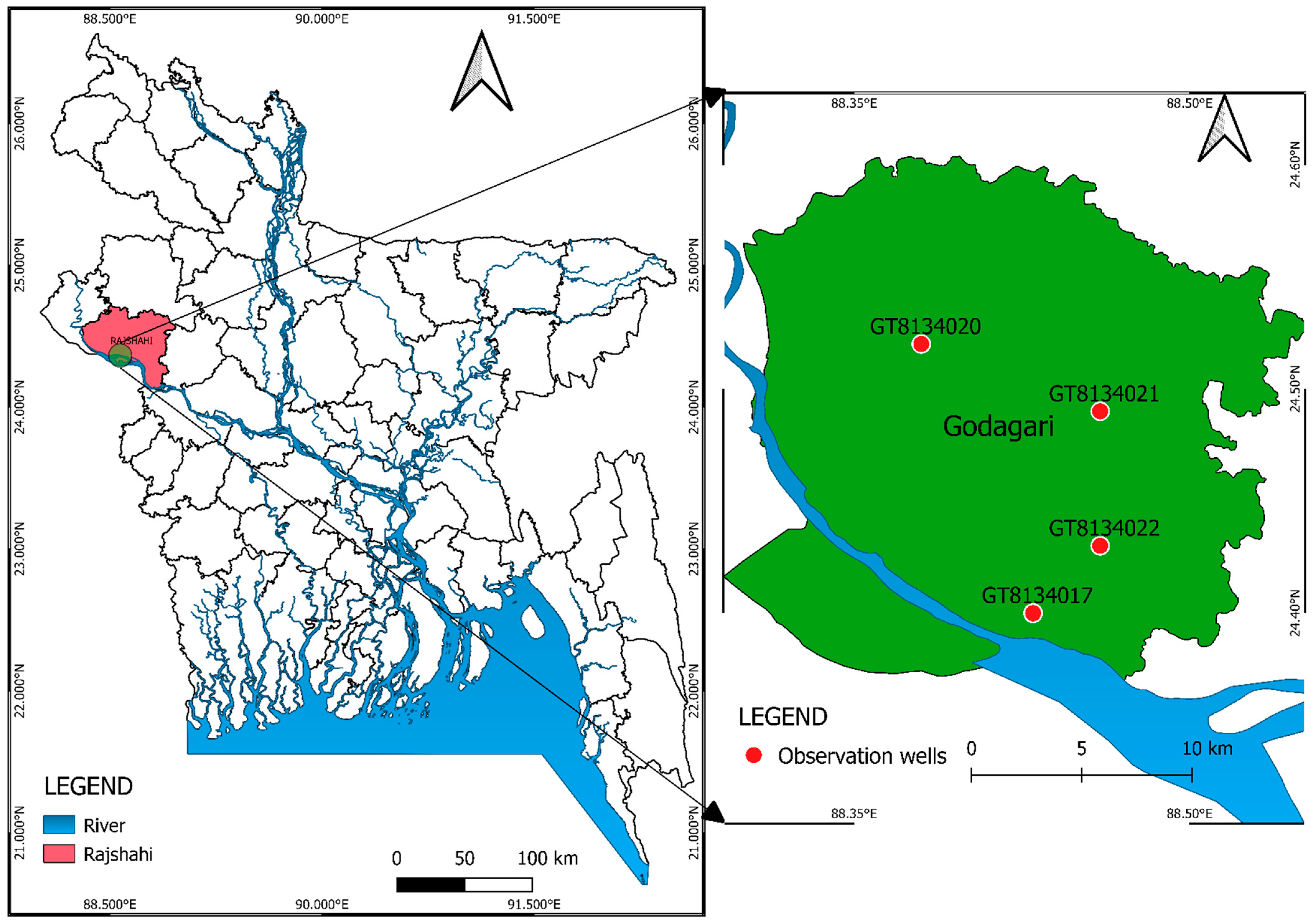
2.1. Study Area and the Data

The study area is located at the Godagari upazilla of the Rajshahi district in the Rajshahi division, Bangladesh. It is situated between 24°21′ and 24°36′ north latitudes and 88°17′ and 88°33′ east longitudes with an aerial extent of about 472.13 km2. The area falls in the extensive Gangetic floodplain, which has a typical climatic pattern with very cold winters (below 6 °C) and very dry and hot summers (up to 45 °C) [34]. It experiences little annual rainfall compared to other parts of the country. Groundwater recharge from rainfall is hindered by a thick clayey layer of around 18 m at the top surface.
Previous data on GWL fluctuations were used to model future scenarios of GWL fluctuations in the selected observation wells of the study area, especially to provide a multi-step ahead forecast of GWLs. For this, weekly historical data on GWL fluctuations with a period from 10 October 1983 to 24 September 2018 (1825 weekly GWL records) were collected from the Bangladesh Water Development Board [35], an entity dedicated to collecting weekly GWL information from designated observation wells. In addition to these GWL records, this organization possesses pump test and lithology data for the observation wells. The research primarily focuses on evaluating the effectiveness of our proposed approach in generating multi-step ahead GWL forecasts with minimal input variables, specifically, utilizing only past GWL data. Our approach eliminates the necessity of incorporating multiple attributes and relying on numerical simulation models, which often demand extensive data and specialized modeling expertise, as well as subjective judgment. In summary, this research relies on secondary data gathered by the Bangladesh Water Development Board, which is responsible for collating water quality and water level data from designated observation wells. This data collection includes manually recorded measurements of the depth of the water level below the ground surface. Collected data at different observation wells were carefully checked and four observation wells, namely GT8134017, GT8134020, GT8134021, and GT8134022, were selected based on the criterion of the least number of missing entries. The observation well GT8134017 is positioned between 24.40° N latitude and 88.43° E longitude. The position of the observation well GT8134020 is between 24.52° N latitude and 88.38° E longitude. The observation well GT8134021 lies between 24.49° N latitude and 88.46° E longitude, whereas the observation well GT8134022 is situated between 24.43° N latitude and 88.46° E longitude. The study area and the positions of the observation wells inside the study area are shown in Figure 1.
To ensure that the collected GWL datasets meet the highest standards, a data quality assurance approach is frequently employed. This approach enhances the reliability of GWL forecasts made using ML techniques. The quality of the collected GWL data was rigorously evaluated for accuracy and completeness using range/limit tests, even though a comprehensive quality inspection method was not applied to the current dataset. The primary objective of range testing is to confirm that each observation falls within a specified range. Only measurements within this threshold are accepted, while those outside of the range are accurately categorized as invalid. To generate a multi-step ahead GWL projection, the data falling within the permissible range were used to model future GWL changes in the selected observation wells.
However, there were some missing values in the GWL datasets in the selected observation wells. The missing entries of weekly GWL data accounted for 0.60% (12 missing entries out of 2021 data), 0.49% (10 missing entries out of 2021 data), 0.35% (7 missing entries out of 2021 data), and 0.39% (8 missing entries out of 2021 data) for the observation wells GT8134017, GT8134020, GT8134021, and GT8134022, respectively. The average of the preceding and subsequent weeks (i.e., adjacent weeks) was used to fill in any gaps in a given week’s data [36]. Table 1 presents a few descriptive statistics of the datasets (after imputation of the missing entries) at the selected observation wells. Table 1 reveals that the mean values of GWL data ranged between 6.534 m (at GT8134022) and 7.735 m (at GT8134020), whereas the standard deviation values varied between 2.274 m (at GT8134022) and 2.797 m (at GT8134017). The data at all observation wells possessed a longer left tail than the right tail in their distribution, as evidenced by the negative skewness values (Table 1). Likewise, the datasets showed “light-tailed” distributions because the kurtosis values are also negative at all observation wells.

2.2. Machine Learning-Based Models

2.2.1. Adaptive Neuro-Fuzzy Inference System (ANFIS)

A hybrid computational model, called the Adaptive Neuro-Fuzzy Inference System (ANFIS), incorporates the advantages of both Artificial Neural Network and fuzzy reasoning methods. Models that can learn from data and then apply that learning to generate predictions or anticipate the future may be developed using ANFIS. The ANFIS model architecture used in this study is Sugeno-based and employs Gaussian and linear-type Membership Functions (MFs) for the inputs and outputs, respectively. According to Jang et al. [37], a Gaussian MF comprises the two important model parameters {c, σ} and can be written as follows:
g a u s s i a n x , c , σ = e 1 2 x c σ 2
where c represents the center of the MF, and σ denotes the MF’s width.
Figure 2 can be used to visually display the architecture of an ANFIS model of the Sugeno-type [37].
The ANFIS architecture depicted in Figure 2 is a basic design that is developed from a Sugeno FIS structure of the first order, comprising a single output ( f ) and two inputs ( α and β ). The fuzzy if-then rules for the Sugeno FIS are represented as:
Rule   1 : If   α   is   P 1   and   β   is   Q 1 then   f 1 = p 1 α + q 1 β + r 1
Rule   2 : If   α   is   P 2   and   β   is   Q 2   then   f 2 = p 2 α + q 2 β + r 2
The ANFIS model is composed of five layers, namely the input layer, fuzzification layer, rule layer, defuzzification layer, and an output layer. The input data is fed into the input layer, and subsequently, the fuzzification layer transforms it into fuzzy sets. Rules are generated in the rule layer based on these fuzzy sets, which are then combined to generate the system output. The defuzzification layer is responsible for converting the fuzzy output to a crisp output. During the learning process, the ANFIS model adjusts the parameters of the fuzzy sets and the rules using the training data. To adjust the parameters of the neural network, the model employs a backpropagation algorithm, while the parameters of the fuzzy sets are adjusted using a least squares method. ANFIS offers several advantages over other modeling techniques due to its ability to handle noisy and uncertain data, capture non-linear relationships between input and output variables, and integrate expert knowledge into the model. The GWL forecasting models based on ANFIS are created by utilizing the functions and commands of MATLAB programming language.
ANFIS employs a hybrid learning algorithm for parameter identification in Sugeno-type fuzzy inference systems (FIS). This approach combines the least squares method and the backpropagation gradient descent method to train FIS membership function parameters, effectively replicating a provided training dataset.
ANFIS models are developed by tuning the parameters of initial FISs, which are created using the fuzzy c-means clustering algorithm (FCM). The FCM is employed to compress the training dataset into a set of identical clusters that significantly reduce the number of rules in FIS generation. This clustering approach substantially reduces the number of adjustable parameters, both linear and nonlinear, within the FIS models. Selecting the optimum number of clusters is an important pre-processing step in FIS model development using the FCM algorithm.
The appropriate number of clusters is determined based on the nature of the problem and the dimension of the input space. In most cases, a simpler model architecture is preferred. In this study, we determine the optimal number of clusters by conducting multiple trials with varying cluster numbers and assessing the resulting Root Mean Square Error (RMSE) between the actual and predicted responses obtained from the selected FIS models. We select the number of clusters that yields the minimum RMSE value and the least variance in RMSE values between the training and testing datasets, considering it to be suitable. We also scrutinize the lowest variance in RMSE values between the training and testing datasets to prevent model overfitting.

2.2.2. Bagged and Boosted RF

A Random Forest (RF) is an ML-based algorithm that utilizes an ensemble of decision trees for making predictions. The method involves generating a group of independent trees and combining their outputs through averaging. Each tree in the forest is constructed based on a random subset of features from the dataset, and the splitting criteria for each tree are determined independently [38]. Bagging and Boosting are commonly utilized in ML to enhance the accuracy of decision tree-based models like RF. These techniques can significantly improve the performance of RF models by reducing model overfitting, variance (in the case of Bagging), and bias (in the case of Boosting). Bagging is a method that entails generating several random samples of the training data by using bootstrapping and training a model on each sample. The ultimate prediction is achieved by taking an average of all the model predictions. This technique helps to mitigate the problem of overfitting and variance that can occur in a model. On the other hand, Boosting is an ML technique that involves training a model on the entire training set and iteratively adjusting the weights of the misclassified samples to enhance the model’s performance. In Boosting, new decision trees are added to the model to correct the errors of the previous trees. The final prediction is made by combining the predictions of all the trees, which are weighted based on their accuracy. A detailed description of the Bagged and Boosted RFs can be found in Breiman [38] and is not repeated in this study. The Bagged-RF and Boosted-RF-based GWL forecasting models are developed using the functions and commands of MATLAB.

2.2.3. Gaussian Process Regression (GPR)

Gaussian Process Regression (GPR) is a non-parametric and Bayesian ML approach that models nonlinear relationships between input and output variables. It uses a Gaussian process, which is a set of random variables that have a joint Gaussian distribution, to model the relationship between inputs and outputs. The goal of GPR is to build a mapping between the predictors, X i and the response variable, Y , expressed as a functional relationship. In simpler terms, GPR is a way to predict outputs based on inputs by building a statistical model using a flexible and non-parametric approach. The functional relationship between X i and Y can be defined as [39]:
Y = f X i + ε
where ε symbolizes the Gaussian noise with variance σ n 2 .
When using GPR, the mean and covariance of the Gaussian process are determined by the data used for training. These two functions play important roles in building the input–output mapping for the GPR model. The mean function is responsible for determining the expected value of the function at any given location in the variable space. In other words, it provides a prediction for the output variable based on the input variables. This mean function can be written as [40]:
m x i = E f x i
The most fundamental and significant component in developing a GPR model is thought to be the covariance function. The covariance function shows how similar or dissimilarly connected the inputs and outputs are. The covariance function is defined as follows:
k x i ,   x j = E   f x i m x i   f x j m x j
A final representation of the Gaussian process is:
f x ~ g p   m x i ,   k x i ,   x j
One of the major benefits of using GPR is that it can effectively model intricate relationships between input and output variables without assuming any specific distribution of the data. This feature is especially useful when dealing with data that may be noisy or incomplete, as GPR cannot only provide predictions but also estimates of the uncertainty associated with these predictions. Therefore, GPR is a powerful tool for predictive modeling in situations where the relationships between variables are complex and the data are imperfect. The GPR-based GWL forecasting models are developed using the functions and commands of MATLAB.

2.2.4. Bidirectional Long Short-Term Memory (Bi-LSTM) Network

Bi-LSTM is a variant of the traditional LSTM neural network, consisting of both forward and backward LSTM layers that allow for the integration of long-range context in both directions. The LSTM architecture addresses the issue of vanishing gradients by using gating mechanisms, while the Bi-LSTM allows for the inclusion of both preceding and subsequent data. The traditional LSTM consists of multiple memory blocks with several memory units and three gates: the input gate selects and converts new data into cell form, the forget gate removes irrelevant information, and the output gate decides which essential information from the cell should be used as the output. As a type of Recurrent Neural Network (RNN), Bi-LSTM transforms the individual activations into dependent activation sequences by providing all neural network layers with identical weights and biases and using prior outputs as input for subsequent hidden layers. In a standard RNN architecture, the hidden layer undergoes an update based on the layer input and prior hidden form at each time step t using the following equation.
h t = σ h   W x t + V h t 1 b h
where W is the weight matrix delivered via the input to the hidden layer, V is the weight matrix between two hidden serial states ( h t 1 and h t ), b h is the bias vector for the hidden layer, and σ h is the activation function to generate the hidden structure. The model output can be represented as
y t = σ y U h t + b y
where U is the weight matrix from the hidden layer converted to the output layer, and σ y is the activation function of the output layer. The LSTM layers process sequential data unidirectionally and modify it to capture the patterns. However, a backward LSTM layer can introduce bidirectional capabilities to the model. The LSTM layers procedure series data unidirectionally and modify it to capture the randomness. Nonetheless, a backward LSTM layer can deliver bidirectionality into the model. Thus, developing a Bi-LSTM layer, including a forward LSTM layer and a backward LSTM layer, processes series data with two particular hidden layers and merges them into the same output layer.
In the development of Bi-LSTM models, network architectures featuring three hidden layers were implemented. Following each of these hidden layers, a dropout layer was incorporated to prevent or mitigate overfitting in the proposed Bi-LSTM models. The first, second, and third hidden layers were configured with 100, 50, and 20 hidden neurons, respectively. Correspondingly, dropout rates of 0.4, 0.3, and 0.2 were assigned to the respective dropout layers. These optimal values were determined through an iterative process of experimentation. Various training configurations for the Bi-LSTM models were explored during these trials and the most effective ones for the model training were selected (Table 2).
The training setup consisted of four layers for the Bi-LSTM models:
  • A sequence input layer, which matched the number of input variables or features.
  • A Bi-LSTM layer, whose units corresponded to the number of hidden units.
  • A fully connected layer, tailored to the number of output variables or response variables.
  • Finally, a regression layer.
This architecture allowed effective training and evaluation of the proposed Bi-LSTM models for the intended task.

2.2.5. Multivariate Adaptive Regression Spline (MARS)

Multivariate Adaptive Regression Spline (MARS) is a non-parametric regression method that was first introduced by Jerome H. Friedman in 1991 [41]. Since then, it has become a widely used technique for modeling intricate and nonlinear relationships between input and output variables in data mining and ML applications. One of the advantages of MARS is its ability to handle both continuous and categorical input variables, as well as their interactions. Additionally, MARS is particularly helpful in identifying the most important input variables in high-dimensional data and modeling non-linear interactions between inputs and outputs. Overall, MARS is a powerful tool for building flexible and accurate regression models in situations where the relationships between variables are complex and nonlinear.
MARS approximates the nonlinear relationship between input and output variables by dividing them into a series of linear segments, which are connected at “knots”. The selection of knots is based on the associated data, and they are used to improve prediction accuracy by minimizing the sum of squared errors between the actual and predicted responses. Each linear segment is represented as a linear combination of the input variables, where the coefficients are also determined by the data.
MARS model building involves both a forward and a backward stepwise procedure. During the forward step, the model is constructed using user-specified Basis functions, while during the backward step, redundant or unnecessary input variables are systematically eliminated to reduce the model’s complexity and prevent over fitting. This results in a more optimal and accurate model. The mapping between input and output variables in MARS can be expressed mathematically, as outlined in Roy and Datta [42].
B F i X = max 0 ,   X j a   o r   B F i X = max 0 ,   α X j
Y = f X = β ± γ k × B F i X
where i and j symbolize the indices for Basic functions and input variables, respectively; B F i indicates the i t h Basis functions; X j denotes the j t h input variables; α is a constant referred to as the knot; β indicates a constant value; γ k represents the corresponding coefficients of B F i X .

2.2.6. Support Vector Regression (SVR)

Support Vector Regression (SVR) is an ML-based approach that is employed for performing regression tasks by offering both linear and non-linear mappings between the input and output variables. It is based on the same principle as Support Vector Machines (SVMs), which are used for classification tasks. The primary goal of SVR is to determine a function that can best approximate the relationship between input and output variables while minimizing the prediction error. To achieve this, SVR maps the input variables to a high-dimensional feature space, where a linear relationship between input and output variables may exist. The technique then identifies a hyperplane that maximizes the margin between the predicted values and the actual values, with the margin represents the distance between the predicted values and the hyperplane. This margin is used to balance the complexity of the model against the error rate. Additionally, SVR is less prone to overfitting than other non-linear regression techniques since it concentrates on discovering the best hyperplane that generalizes well to new data [43]. This effort provides a concise overview of how SVR models can be used to solve regression problems. When constructing an SVR model, the training dataset can be expressed using the following equation:
P = a 1 , b 1 , a 2 , b 2 , a 3 , b 3 , . , a N , b N
where a i i = 1 , 2 , 3 , . , N represents a vector comprising real independent variables; b i i = 1 , 2 , 3 , . , N represents the associated scalar real independent variable. The feature space representation of the regression equation for the training dataset is as follows:
z a , w = w · a + c
where w represents the weight vector; c symbolizes a constant; a denotes the feature function; and w · a represents the dot product. SVR minimizes the following cost function to accomplish regression tasks:
Minimize :   Q f = C 1 N L ε b , z a , w + 1 2 W 2
L ε b , z a , w = 0 if     b z a , w ε   b z a , w ε otherwise
The above equation represents the empirical error, while the second term (denoted by C ) measures the trade-off between the empirical error and the model complexity. Equation (15) represents a loss function referred to as the “ε-insensitive loss function” [44]. By introducing Lagrangian multipliers β and β * , the optimization problem in Equation (15) is transformed into a dual problem.
Support vectors are only defined as combinations of non-zero coefficients and their corresponding input vectors, a i . The equation eventually has the following final form:
z a , β i , β i * = i = 1 N s v β i β i * a i · a j + c
The SVR function can be expressed as follows using the kernel function K x i , x j :
z a , β i , β i * = i = 1 N s v β i β i * K a , a i + c
The above equations are used to compute the term c using the Karush–Kuhn–Tucker condition. When using the SVR technique to solve a regression problem, the cost function C , the radius of the insensitive tube ε , and the kernel parameters K x i , x j are thought to be the most crucial variables. The forecasting models for GWL based on the SVR approach are developed using MATLAB’s functions and commands.

2.3. Modeling Techniques

This section provides specifics on data pre-processing and modeling techniques adopted in this research to develop the ML-based forecast models (ANFIS, Bagged RF, Boosted RF, GPR, Bi-LSTM, MARS, and SVR) proposed in this research to forecast multi-step ahead GWL fluctuations.
Data pre-processing is a crucial step in enhancing the forecasting accuracy of any ML model. It encompasses various tasks, including data collection and compilation, quality assessment, cleaning and imputation, data splitting, feature engineering, and data standardization, among others, to ensure that the data are suitable for analysis and modeling. The issues related to data collection and compilation, as well as cleaning and imputation, are addressed in Section 2.1, ‘Study area and the data’. Subsequent sub-sections provide detailed information on data splitting, feature engineering, data standardization, and the modeling techniques employed in this research. These steps collectively contribute to improving the forecasting accuracy of multi-scale GWL fluctuations using a heterogeneous ensemble of ML algorithms.

2.3.1. Data Preprocessing

Initially, a total of 1825 GWL records (from 10 October 1983 to 24 September 2018) were collected for providing multi-step ahead GWL forecasts. The collected weekly GWL data decreased at every observation well due to temporal lags for the lagged inputs and the output. At each observation well, a total of 1807 historical records remained (from 13 February 1988 to 24 September 2018 after removing 18 records due to time lagging (3-time lags forward + 15-time lags backward) from the entire GWL time series of 1825 readings (from 10 October 1983 to 24 September 2018). The remaining dataset at each observation well were divided into three subsets: the first 1267 datasets (70% of total) were employed for model development (training), the next 270 datasets (15% of total) were used for model validation, and the remaining 270 datasets (15% of total) were used for model evaluation (testing). After satisfactory training and validation of the GWL forecast models, the models were tested using an unseen test dataset, which was used neither for model training nor for model validation. Although there is not a fixed rule for dataset dividing throughout model training and validation [45], it is generally agreed that the validation division should be between 10% and 40% of the length of the entire dataset [46].

2.3.2. Selection of Input Variables

One of the most crucial aspects in creating ML-based forecast models is deciding on the influential input variables [47,48]. In order to choose the input variables for hydrological and water resources modeling, both linear [49] and nonlinear approaches [48] have been used [47]. However, because hydrological and water resource modeling frequently involves nonlinear issues, linear approaches based on the Partial Auto Correlation Function (PACF) and Auto Correlation Function (ACF) are normally not the best approaches [50]. In general, nonlinear approaches based on Mutual Information (MI) [51] outperform linear approaches for the modeling of hydrology and water resources research areas in addition to other scientific and technological application domains [32,47,48,52]. Since ANFIS, GPR, Bi-LSTM, and SVR do not automatically quantify the significance of input variables, it is crucial to undertake the selection of most influential input variables before developing these models. In this research, we employed the Minimum Redundancy Maximum Relevance (MRMR) technique developed by Peng et al. [53], one of the most popular MI techniques for input variable identification. Using MI to find potential candidate inputs that are pertinent but not unnecessary, this method chooses input variables from a group of alternatives. It has been demonstrated that this method chooses input variables that are more suitable than other methods of a similar kind [54]. An operator Φ D , R is defined to concurrently optimize the minimum redundancy ( R ) and maximum relevance ( D ) for selecting an input subset ( S ) from d input variables in x [53]. This can be mathematically represented as:
max Φ D , R ,   Φ = D R
A detailed outline of MRMR can be found in Peng et al. [53] and is not repeated in this effort. Nevertheless, for approaches like MARS and RF, the choice of the input variable is not required. Both strategies carry out the internal functions of input variable selection and variable importance quantification.

2.3.3. Standardization of Data

Data standardization is seen as a method for putting data on a uniform scale, making them simpler to assess and compare. In order to be certain that various variables or attributes are on an equivalent scale and have identical ranges, machine learning algorithms are standardized. In the present investigation, the variables used for input were initially normalized before the GWL forecasting models were built. Several earlier studies on hydrology and water resources used the standardization approach [55,56]. As a result, the dataset was created with a mean of 0 and a variance of 1 [57]. The data were standardized using the following formula:
X s t a n d a r d i z e d = X μ σ
where X represents the actual input, X s t a n d a r d i z e d denotes the standardized input, μ is the mean value of the input, and σ is the standard deviation of the input.

2.3.4. Development of Individual Models

The choice of the best parameter settings has a significant impact on how accurately the majority of ML-based algorithms forecast. Probst et al. [58] claim that the vast majority of ML algorithms require that a set of properly selected appropriate parameters be used. ML-based model performance is significantly influenced by the choice of parameters [59], and poor parameter choosing can lead to underachieving models. To enable an equitable evaluation of ML-based forecasting models, it is ideal to choose the best or optimal parameter sets for each of the ML-based models. In this attempt, a number of trials were run using different parameter sets for each model in order to pick the best models using the best parameter values for that model. The training and validation data were used to conduct these trials, which examined the RMSE of the training phase and validation performance. When the RMSE values for the training and validation phases differed very little from one another, it was determined that a model was performing at its peak efficiency and that no model was overfitted. The parameters that were used for the trained individual GWL forecast models developed at the four observation wells are shown in Table 2.

2.3.5. Development of Ensemble Models

Different ML-based modeling approaches have varying degrees of precision in forecasting. In accordance with the datasets utilized in both training and evaluation, the efficacy of a model may change. It is important to select the best model for a specific problem; not all ML-based modeling techniques can be used in a given study to compare the effectiveness of each one. This selecting process is difficult and time-consuming. An ensemble modeling technique has a benefit in these circumstances because it enables the selection of a predetermined number of effective models and the combination of their forecasts to provide more precise outcomes. An ensemble forecast enhances forecast reliability by more accurately capturing the relationships between the predictors and responses in the dataset. Additionally, it shields a model’s performance from an individual poor model by minimizing the impact of poor projections from the model in question [60]. An ensemble technique utilizes the unique characteristics of individual models to recognize various input–output relationship trends across the whole decision space of the input–output data. For this reason, ensemble models frequently provide higher precision than an individual forecast model. Individual forecasting models used in the ensemble development must, however, be sufficiently precise and varied to be useful for forecasting. The appropriate balance between independent forecasting models in an ensemble-based forecast is mostly governed by the trade-offs between model complexity, forecasting accuracy, and the level of uncertainty minimization.
To overcome the limitations of the forecast performance of the individual models, the present study utilizes a weighted average ensemble approach using the BMA approach [61]. When there is ambiguity over the best model to utilize, BMA is a statistical method that is employed to calculate the parameters of the model and generate forecasts. BMA, which combines forecasts from many different models by weighing them in accordance with their posterior probabilities, which are determined using the data at hand and a prior distribution over the models in question, offers an improved comprehension of the overall forecasting uncertainty [62]. In order to derive consensus predictions, BMA uses probabilistic probability measures for weighting individual predictions, with higher probability likelihood values obtaining bigger weights than forecasts that have lower probability likelihood values. The fundamental tenet of BMA is to approach model selection as a random variable and to account for this uncertainty in the analysis. BMA takes into account a set of candidate models and assigns a probability to each one depending on how well it fits the data and how well it relates to prior knowledge about the problem, rather than choosing a single “best” model based on some criterion (e.g., statistical performance assessment indices). In comparison to individual ensemble members created using several competing ML algorithms, BMA offers a probabilistic forecast that offers more accuracy and dependability [62]. For challenges involving multi-scale GWL prediction, the BMA technique was employed in this endeavor. A thorough description of the BMA approach can be found in the literature [61,62,63], hence the following is a concise summary of it.
Let us consider the following terms and notations: y denotes the predicted variable, D = y 1 o b s e r v e d ,   y 2 o b s e r v e d , y 3 o b s e r v e d , , y N o b s e r v e d represents the training data with a data length of N , and f = f 1 , f 2 , f 3 , , f k is the ensemble of all selected individual model predictions. Furthermore, consider p k y | f k , D to be the posterior distribution of y with model prediction f k and matrix of the training data D . Then, according to the total probability law, the Probability Density Function (PDF) of the BMA-based probabilistic prediction of y is presented using the equation below:
p y | D = k = 1 K p f k | D · p k y | f k , D
where p f k | D denotes the posterior probability of the model prediction f k , also known as the probability of model prediction f k being the accurate prediction for the training data set D . The term p f k | D in Equation (20) determines how precisely this specific ensemble member matches the actual observed values. If we consider the term p f k | D to be equal to the weights of the individual ensemble member, i.e., w k = p f k | D , then the sum of weights for all individual ensemble members should be equal to 1, i.e., k = 1 K w k = 1 . The BMA predictions’ posterior mean and variance can be represented by the following equations [62]:
E y | D = k = 1 K p f k | D · E p k y | f k , D = k = 1 K w k f k
Var y | D = k = 1 K w k f k i = 1 K w i f i 2 + k = 1 K w k σ k 2
where σ k 2 denotes the variance related to the model prediction f k concerning the training data set D . The expected BMA forecast is essentially the average of the various predictions weighted by the probability that a particular model is accurate for the given observations.
In the BMA algorithm, it is assumed that the conditional probability distribution, denoted as p k y | f k , D , follows a Gaussian distribution. In the standard BMA approach, the EM algorithm is employed to maximize the log-likelihood function associated with the parameter vector being estimated. If we represent θ as θ = w k , σ k , k = 1 , 2 , , K , the log-likelihood function can be approximated as follows:
l θ = log k = 1 K w k . p k y | f k , D
Obtaining an analytical solution for this problem is infeasible, necessitating the use of an iterative procedure. The EM algorithm is particularly well suited for this purpose. In essence, the EM algorithm formulates the maximum likelihood problem as a ‘missing data’ problem. This missing data may not represent actual observations but can instead be a latent variable that requires estimation. It is important to note that the EM algorithm tends to converge to local optima, and the optimal solution is highly sensitive to the initial guess of the optimization variables. For clarity, Figure 3 illustrates a flow diagram of the proposed ensemble model, including the algorithmic flow of the execution of the EM algorithm.
Since the probability of a model is essentially a gauge of how well the model forecasts match the data provided, one benefit of BMA is that a BMA forecast is given larger weights from models that perform better. Another benefit of BMA is that it offers a means to account for model uncertainty (through BMA variance) and prevent overfitting, which can happen when a single model is chosen based on a particular criterion. BMA variance is made up of two parts: (1) between-model variance, which is expressed by the very first component on the right-hand side of the equation (Equation (22)); and (2) within-model variance, which is indicated by the second component on the right-hand side of the equation (Equation (22)). As a result, BMA offers a more accurate representation of predictive uncertainty than a non-BMA-based ensemble strategy, which integrates uncertainty based solely on the ensemble spread (considers between-model variance alone), and on the other hand, produces under-dispersive predictions [62].
With the proper estimation of θ = w k , σ k , k = 1 , 2 , , K and p k y | f k , θ , D , it is possible to easily generate probabilistic forecasts using Equation (20).

2.4. Model Performance Evaluation

Correlation Coefficient (R) [64]:
R = i = 1 n G W L i , A G W L A ¯ G W L i , A G W L P ¯ i = 1 n G W L i , A G W L A ¯ 2 i = 1 n G W L i , P G W L P ¯ 2
Root Mean Squared Error (RMSE) [65]:
R M S E = 1 n i = 1 n G W L i , A G W L i , P 2
Normalized RMSE (NRMSE) [66]:
N R M S E = R M S E G W L A ¯
Mean Absolute Error (MAE):
M A E = mean G W L i , A G W L i , P
Mean Absolute Deviation (MAD) [67]:
M A D H G W A , G W L P = m e d i a n ( G W L A ,   i = 1 G W L P ,   i = 1 , | G W L A ,   i = 2 G W L P ,   i = 2 | , , H G W A ,   i = n G W L P ,   i = n   )   f o r   i = 1 , 2 , , n
Willmott’s Index of Agreement (IOA) [68]:
I O A = 1 i = 1 n G W L i , A G W L i , P 2 i = 1 n G W L i , P G W L A ¯ + G W L i , A G W L A ¯ 2
Nash–Sutcliffe Efficiency Coefficient (NS) [69]:
N S = 1 i = 1 n G W L i , A G W L i , P 2 i = 1 n G W L i , A G W L A ¯ 2
Mean Bias Error (MBE) [70]:
M B E = 1 n i = 1 n G W L i , P G W L i , A
a20index:
a 20 i n d e x = K 20 n
where G W L i , A = actual groundwater level values, G W L i , P = predicted groundwater level values, G W L A ¯ = mean of the groundwater level values, G W L P ¯ = mean of the forecasted groundwater levels, S D represents the standard deviation of the observed data, n = number of samples (GWL data), and K 20 = number of test samples that have a G W L i , A / G W L i , P ranging between 0.80 and 1.20. The a 20 i n d e x quantifies the number of forecasts that have a ratio of actual and forecasted values within a range of 0.80 and 1.20.

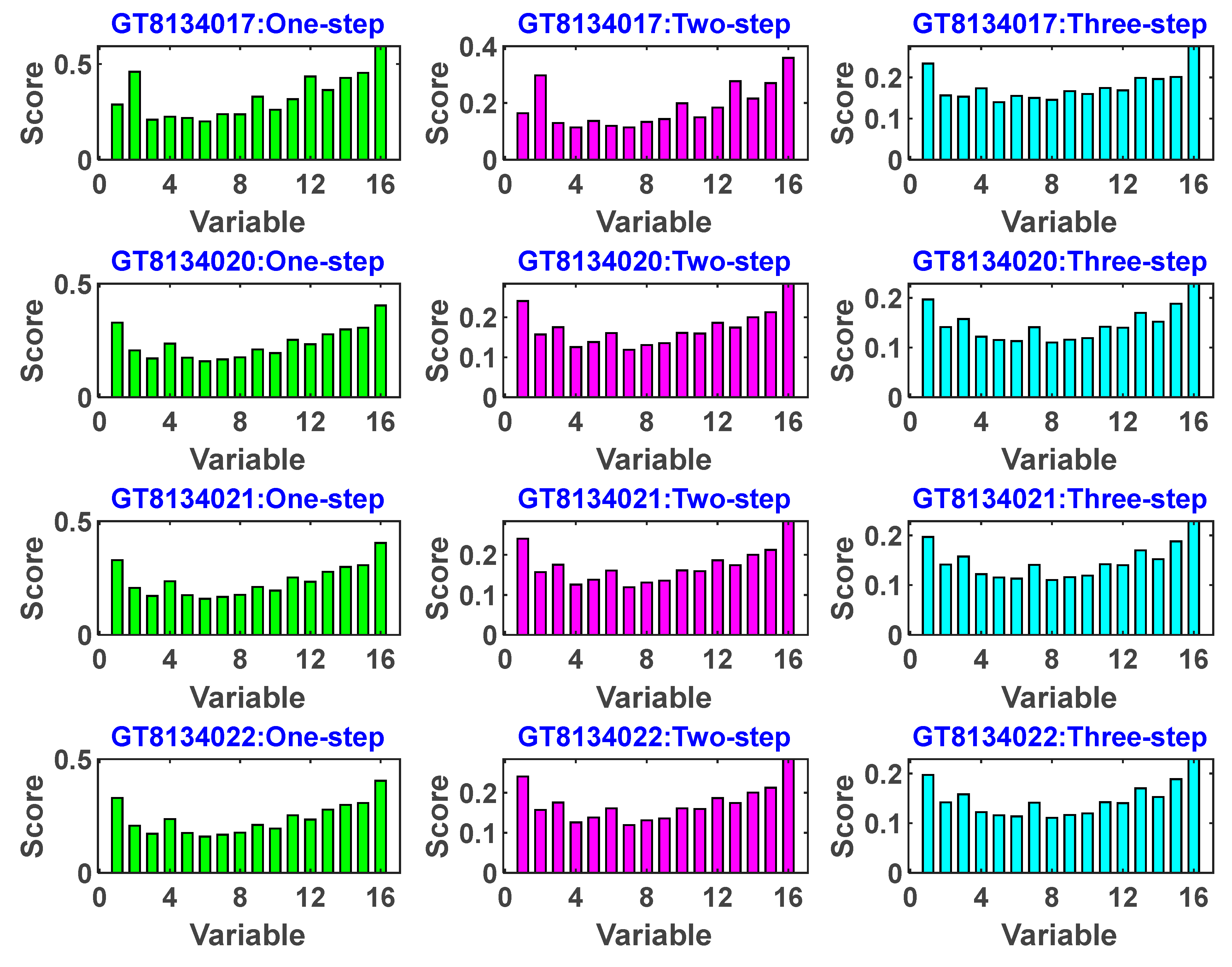
2.5. Variable Importance

MARS and RF variants (Bagged and Boosted RF) inherently offer insights into the significance of explanatory variables for predicting the target variable. For other models, a total of sixteen (GWL at present time and 15 lags behind) most significant input variables were selected using the MRMR technique presented in Section 2.3.2. The feature importance score was computed and the top 16 predictors were selected for the one-, two-, and three-steps ahead forecasts individually at the four observation wells. A high score value indicates the significance of the associated predictor. Likewise, a reduction in the feature importance score reflects the level of confidence in feature selection. For instance, if the MRMR technique confidently selects feature x , the score value of the subsequent important feature would be notably lower than that of feature x . Given that there was no considerable disparity between the scores of the subsequent predictors until the sixteenth most significant predictors, we opted for the first sixteen most important features to build the ML-based models. The analysis revealed that certain variables exhibit substantial relative contributions to the models, while the majority displayed minimal or negligible contributions. It was generally observed that lagged GWL (Lag-1), as expected, was the most important variable for 1 week ahead forecasting (Figure 4).

3. Results and Discussion

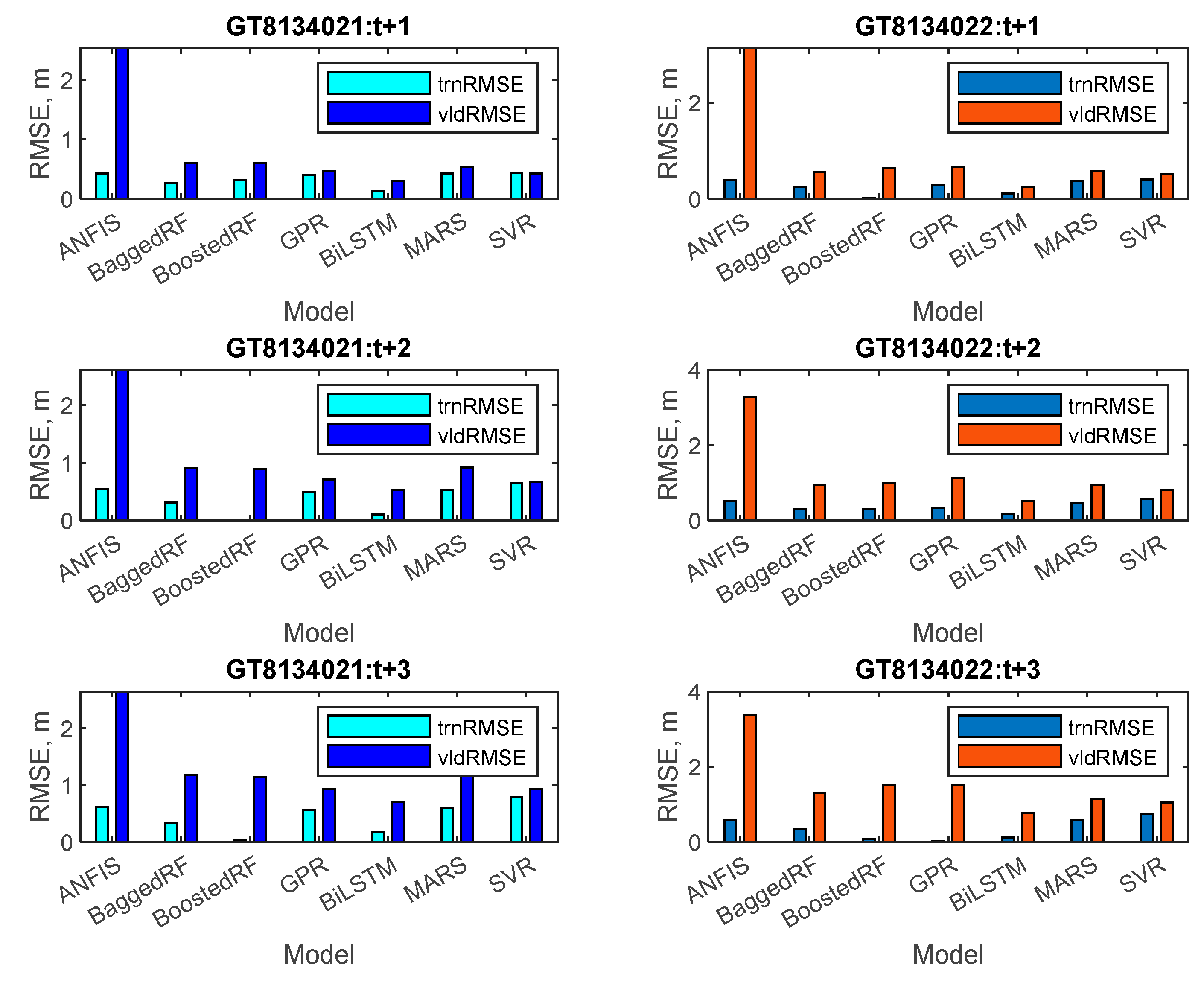
3.1. Performance of the Individual Forecasting Models during Training and Validation

Training and validation were carried out for the individual forecasting models to assess their performance. Figure 5 and Figure 6 display the RMSE index, utilized to compare the efficiency of the proposed models across the learning and validation phases. The RMSE values for various standalone models forecasting GWL one, two, and three weeks in advance are presented for both the learning and validation datasets. This index serves as a metric for gauging the accuracy of the models during their development. The results reveal that, in the cases of wells GT8134017, GT8134021, and GT8134022, the SVR model exhibited lesser disparities between RMSE values in training and validation, in contrast to other models like ANFIS, BaggedRF, BoostedRF, GPR, BiLSTM, and MARS, which demonstrated more significant discrepancies. Conversely, for well GT8134020, the MARS model showcased a smaller variance, while ANFIS, BaggedRF, BoostedRF, GPR, BiLSTM, and SVR displayed higher divergences. Of all the models, ANFIS displayed the weakest performance, yielding the most notable dissimilarities in terms of RMSE values between the training and validation phases.

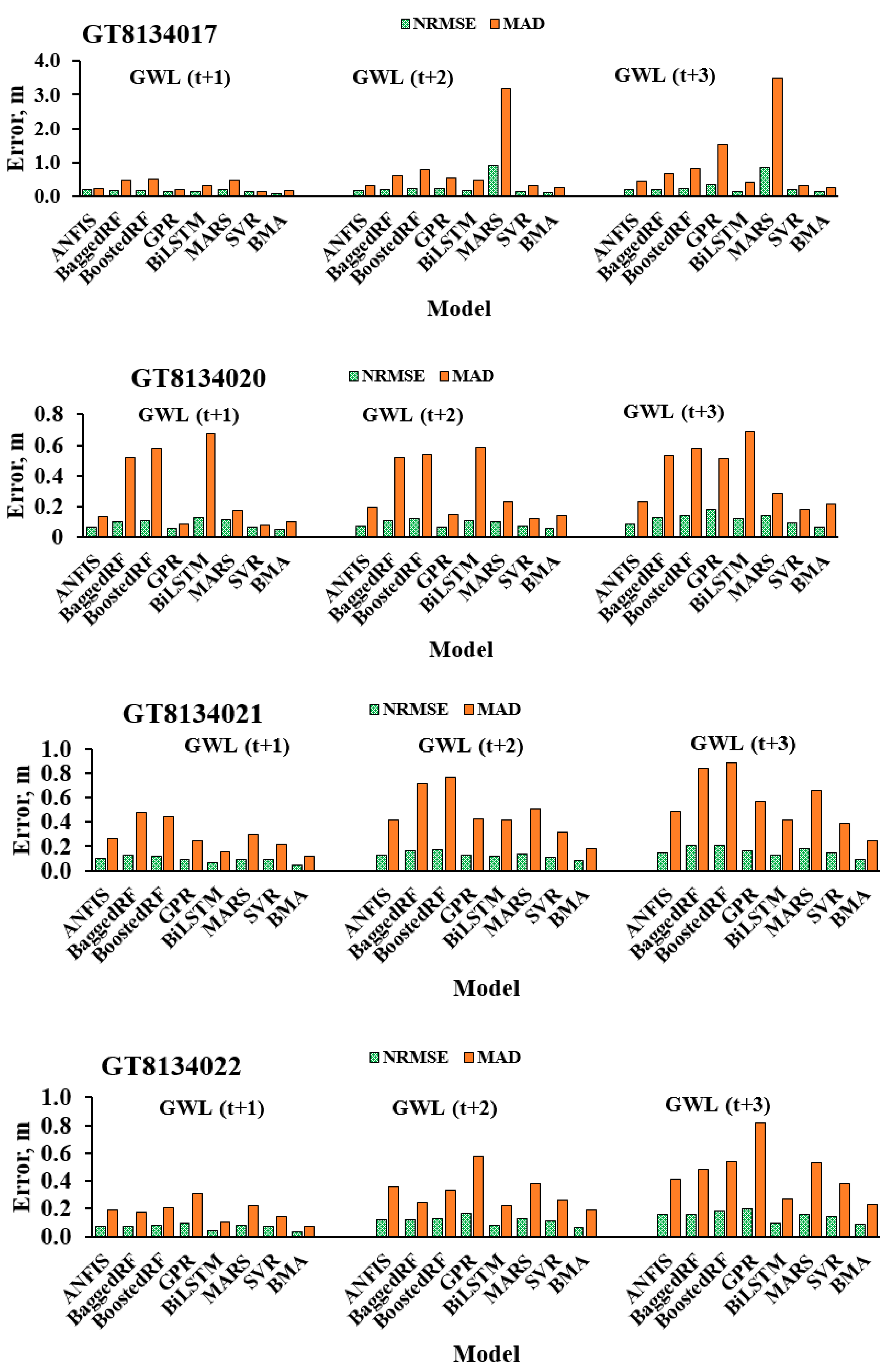
3.2. Performance of the Standalone and Ensemble Models on the Independent Test Dataset

When applied as individual models, ML-based models often struggle to capture the wide range of complex patterns contained in the dataset. This limitation can lead to poor predictions. In such situations, an ensemble of standalone prediction models can be employed, which sometimes outperforms an individual model [24]. Therefore, due to the frequent inability of standalone forecast models to capture the true trends within training and testing patterns of the dataset, the concept of ensemble prediction has been introduced in this research. Furthermore, efforts in model development typically focus on reducing prediction uncertainties to provide meaningful predictions and enhance the generalization capacity of the developed models. This can be accomplished by integrating the predictions of multiple standalone models, creating an ensemble of models that produces a single combined prediction [60].
An ensemble approach can be either homogeneous or heterogeneous, depending on the use of single or multiple ML-based algorithms in the ensemble formation [24]. Previous studies on GWL prediction have demonstrated the effectiveness of homogeneous ensembles [29], which outperformed standalone models. Although recent studies on saltwater intrusion problems in coastal aquifers have applied a heterogeneous ensemble of prediction models [24], this approach has not been previously employed to enhance the forecasting accuracy of multi-scale GWL forecasts. This study examines the application of a BMA-based ensemble approach to enhance the accuracy and reliability of multi-scale GWL forecasts. The approach involves consolidating multiple competing forecasts generated by various ML algorithms. BMA is a statistical method that derives consensus predictions by assigning weights to individual predictions based on their probabilistic likelihood measures. Predictions with superior performance receive greater weights than those with poorer performance. Additionally, BMA offers a more dependable representation of the overall predictive uncertainty compared to the other ensemble approaches, resulting in a more precise and well-calibrated Probability Density Function (PDF) for the probabilistic predictions.
Ensemble techniques aim to enhance the accuracy and consistency of predictions by amalgamating multiple standalone forecast models. The rationale underlying ensemble forecasting rests upon the notion that diverse models possess individual strengths and weaknesses. By consolidating their predictions, a more resilient and precise ML-based algorithm can be crafted. Ensemble forecasting is a widely favored strategy to amalgamate the forecasting accuracies of individual models due to their divergent performances in varied scenarios [24]. A comprehensive comparison between the performances of independent models and the BMA ensemble approach distinctly showcases the supremacy of the BMA methodology across the GT8134017, GT8134020, GT8134021, and GT8134022 observation wells. It is worth noting that the precision of forecasts, as gauged by evaluation indices, diminishes as forecasting horizons extend. In essence, one-week forecasts outperformed two-week forecasts, and two-week forecasts exhibit greater accuracy than three-week forecasts.
Figure 7 and Figure 8 illustrate the individual model performances across various statistical indices when predicting the weekly GWL of four observation wells. In Figure 7, the NRMSE and MAD values for various ML-based algorithms are presented across different observation wells. In terms of statistical significance, the accuracy of a model improves as the NRMSE and MAD values decrease. At the GT8134017 well, the BMA model emerged as the highest-ranking model, showcasing lower NRMSE values (0.09, 0.12, and 0.13 for one-, two-, and three-week ahead GWL forecasts) as well as lower MAD values (0.17, 0.25, and 0.27 for one-, two-, and three-week ahead GWL forecasts). Conversely, the MARS model exhibited the poorest performance, characterized by higher NRMSE and MAD values (NRMSE = 0.20, 0.91, and 0.85; MAD = 0.48, 3.18, 3.48 for one-, two-, and three-week ahead GWL forecasts). Similarly, across the GT8134020, GT8134021, and GT8134022 wells, the BMA model consistently demonstrated lower NRMSE and MAD values, further confirming its favorable performance.
Conversely, depicted in Figure 8 are the values of R, IOA, and a-20 index for distinct ML-based algorithms across various observation wells. Broadly, heightened values of R, IOA, and a-20 index correspond to enhanced model accuracy. For the GT8134017 observation well, BMA exhibited superior performance when compared to alternative models, as evidenced by its higher values of R (0.93, 0.88, and 0.86), IOA (0.96, 0.93, and 0.92), and a-20 index (0.94, 0.91, and 0.91) for one-, two-, and three-week ahead GWL forecasts, respectively. Likewise, BMA consistently outperformed other models across the remaining observation wells, corroborating its efficacy. The findings presented in Figure 7 and Figure 8 collectively indicate that the BMA model emerges as the superior choice across various prediction horizons for different observation wells, surpassing other standalone models when evaluated on the independent test dataset.
In this study, the BMA approach exhibits exceptional performance, with larger R, IOA, and a-20 index values and smaller NRMSE and MAD values across all three forecasting horizons and the four observation wells. For instance, at the GT8134017 observation well, the BMA model improves the accuracy of statistical indices in one-week forecasts by (R = 25.67%, NRMSE = 55%, MAD = 68%, IOA = 15.67%, and a-20 index = 18.98%) compared to the poorest-performing model. On average, the BMA model consistently demonstrates greater accuracy than other individual models across other observation wells. According to our study, the BMA approach offers a more dependable and robust comprehension of overall predictive uncertainty.
The effectiveness of the proposed Bayesian Model Averaging approach over the independent models is also apparent when considering other statistical performance evaluation measures, as presented in Table 3. It is evident from the data presented in Table 3 that, despite the individual models yielding comparatively reduced Root Mean Squared Error, Mean Absolute Error, and Mean Bias Error values, the Bayesian Model Averaging approach consistently yields the most minimized values across all observation wells and forecasting horizons. While the standalone models exhibit relatively lower Nash–Sutcliffe Efficiency Coefficient values, the Bayesian Model Averaging approach consistently outperforms them in terms of NS for all instances.
A noteworthy observation is that the forecasting performance decreases as the forecasting horizon extends. This finding aligns well with the conclusions drawn by Rahman et al. [71] and Quilty et al. [48], who reported that the accuracy of predictive models tends to decrease with the expansion of the forecasting horizon. In summary, the suggested heterogeneous ensemble of forecast models based on Bayesian Model Averaging has substantially enhanced the reliability and accuracy of multi-scale groundwater level fluctuations within the study area. This result aligns well with the conclusions reported by Darbandsari and Coulibaly [72].

4. Conclusions

A dependable and precise forecast of GWLs can be used to create a groundwater management strategy that is effective and sustainable. For agricultural, household, and industrial uses, this planning will help to determine the best groundwater abstraction recommendations. But it is frequently challenging to provide precise GWL forecasts because of the nonlinear nature of GWLs as well as their multi-scale and time-varying behavior. An essential requirement for building precise ML-based models involves the selection of the most pertinent input variables from a pool of potential candidates, in conjunction with the optimization of model parameters. To tackle these concerns, this study evaluated the efficacy of various ML-based approaches capable of effectively capturing nonlinear relationships between input and output variables and that often show the best accuracy for GWL and other research domains in different parts of the world. Few of the ML-based approaches are able to perform selection of the most significant input variables internally, while for the others, the most significant input variables were selected using the MRMR approach. These models were fed into the time-lagged information extracted from the time series data. Furthermore, these ML-based forecasting model outputs were integrated using the BMA approach to enhance the forecasting models’ ability. The proposed models were explored for 1, 2, and 3 weeks ahead GWL forecasting. The performance of the proposed BMA approach was compared against standalone forecast models.
The comparison between individual ML approaches and their heterogeneous ensemble (BMA) counterpart demonstrated that the BMA approach exhibited higher accuracy in comparison to the standalone ML models. The standalone ML methods also showcased respectable accuracy, albeit slightly below the level achieved by the BMA approach. Evaluation indices consistently highlighted the outstanding performance of the suggested BMA-based heterogeneous ensemble technique, even though performance marginally declined as forecast horizons increased. The ensemble approach based on BMA notably enhanced the accuracy of GWL forecasts across various lead times, with particularly notable improvement for 1-week ahead forecasts than the 2- and 3-week ahead forecasts at the observation wells. This outcome holds promise for forecasting multi-scale processes frequently encountered in hydrology and water resources. The amalgamation of ML methods through the BMA approach presents a compelling novel framework for GWL forecasting in the study area, warranting further exploration in the realm of hydrology and water resources, both for short-term and long-term predictive applications. It is worth mentioning that this study utilized a dataset covering roughly 35 years, ranging from 1983 to 2018. Further validation of the proposed modeling approach can be conducted using the most recent dataset obtained from the selected observation wells and potentially applied in a future study.

Author Contributions

Conceptualization, methodology, formal analysis, software, validation, visualization, writing—original draft, D.K.R. and N.A.-A.; data curation, project administration, investigation, writing—review and editing, T.H.M., C.R.P., M.P.H., N.A.-A. and M.A.M. All authors have read and agreed to the published version of the manuscript.

Funding

Researchers Supporting Project number (RSPD2023R958), King Saud University, Riyadh, Saudi Arabia.

Data Availability Statement

Not applicable.

Acknowledgments

The authors would like to thank Researchers Supporting Project number (RSPD2023R958), King Saud University, Riyadh, Saudi Arabia.

Conflicts of Interest

The authors declare no conflict of interest.

References

  1. Hasan, M.R.; Mostafa, M.; Rahman, N.; Islam, S.; Islam, M. Groundwater Depletion and Its Sustainable Management in Barind Tract of Bangladesh. Res. J. Environ. Sci. 2018, 12, 247–255. [Google Scholar] [CrossRef]
  2. Monir, M.; Sarker, S.; Sarkar, S.K.; Mohd, A.; Mallick, J.; Islam, A.R.M.T. Spatiotemporal Depletion of Groundwater Level in a Drought-Prone Rangpur District, Northern Region of Bangladesh. 21 June 2022; PREPRINT (Version 1). [Google Scholar] [CrossRef]
  3. Murphy, J.; Sexton, D.; Barnett, D.; Jones, G.; Webb, M.; Collins, M.; Stainforth, D. Quantification of Modelling Uncertainties in a Large Ensemble of Climate Change Simulations. Nature 2004, 430, 768–772. [Google Scholar] [CrossRef] [PubMed]
  4. Ewen, J.; O’Donnell, G.; Burton, A.; O’Connell, E. Errors and Uncertainty in Physically-Basedrainfall-Runoff Modeling of Catchment Change Effects. J. Hydrol. 2006, 330, 641–650. [Google Scholar] [CrossRef]
  5. Vu, M.; Jardani, A.A.; Massei, N.; Fournier, M. Reconstruction of Missing Groundwater Level Data by Using Long Short-Term Memory (LSTM) Deep Neural Network. J. Hydrol. 2020, 597, 125776. [Google Scholar] [CrossRef]
  6. Pham, Q.; Kumar, M.; Di Nunno, F.; Elbeltagi, A.; Granata, F.; Islam, A.R.M.T.; Talukdar, S.; Nguyen, X.; Najah, A.-M.; Tran Anh, D. Groundwater Level Prediction Using Machine Learning Algorithms in a Drought-Prone Area. Neural Comput. Appl. 2022, 34, 10751–10773. [Google Scholar] [CrossRef]
  7. Jeong, J.; Park, E. Comparative Applications of Data-Driven Models Representing Water Table Fluctuations. J. Hydrol. 2019, 572, 261–273. [Google Scholar] [CrossRef]
  8. Sun, J.; Hu, L.; Li, D.; Sun, K.; Yang, Z. Data-Driven Models for Accurate Groundwater Level Prediction and Their Practical Significance in Groundwater Management. J. Hydrol. 2022, 608, 127630. [Google Scholar] [CrossRef]
  9. Zanotti, C.; Rotiroti, M.; Sterlacchini, S.; Cappellini, G.; Fumagalli, L.; Stefania, G.A.; Nannucci, M.S.; Leoni, B.; Bonomi, T. Choosing between Linear and Nonlinear Models and Avoiding Overfitting for Short and Long Term Groundwater Level Forecasting in a Linear System. J. Hydrol. 2019, 578, 124015. [Google Scholar] [CrossRef]
  10. Vadiati, M.; Yami, Z.; Eskandari, E.; Nakhaei, M.; Kisi, O. Application of Artificial Intelligence Models for Prediction of Groundwater Level Fluctuations: Case Study (Tehran-Karaj Alluvial Aquifer). Environ. Monit. Assess. 2022, 194, 619. [Google Scholar] [CrossRef]
  11. Jafari, M.M.; Ojaghlou, H.; Zare, M.; Schumann, G.J. Application of a Novel Hybrid Wavelet-ANFIS/Fuzzy c-Means Clustering Model to Predict Groundwater Fluctuations. Atmosphere 2021, 12, 9. [Google Scholar] [CrossRef]
  12. Che Nordin, N.F.; Mohd, N.S.; Koting, S.; Ismail, Z.; Sherif, M.; El-Shafie, A. Groundwater Quality Forecasting Modelling Using Artificial Intelligence: A Review. Groundw. Sustain. Dev. 2021, 14, 100643. [Google Scholar] [CrossRef]
  13. Kombo, O.; Santhi, K.; Sheikh, Y.; Bovim, A.; Jayavel, K. Long-Term Groundwater Level Prediction Model Based on Hybrid KNN-RF Technique. Hydrology 2020, 7, 59. [Google Scholar] [CrossRef]
  14. Tian, Y.; Xu, Y.-P.; Yang, Z.; Wang, G.; Zhu, Q. Integration of a Parsimonious Hydrological Model with Recurrent Neural Networks for Improved Streamflow Forecasting. Water 2018, 10, 1655. [Google Scholar] [CrossRef]
  15. Ebrahimy, H.; Feizizadeh, B.; Salmani, S.; Azadi, H. A Comparative Study of Land Subsidence Susceptibility Mapping of Tasuj Plane, Iran, Using Boosted Regression Tree, Random Forest and Classification and Regression Tree Methods. Environ. Earth Sci. 2020, 79, 223. [Google Scholar] [CrossRef]
  16. Arabameri, A.; Yamani, M.; Pradhan, B.; Melesse, A.; Shirani, K.; Tien Bui, D. Novel Ensembles of COPRAS Multi-Criteria Decision-Making with Logistic Regression, Boosted Regression Tree, and Random Forest for Spatial Prediction of Gully Erosion Susceptibility. Sci. Total Environ. 2019, 688, 903–916. [Google Scholar] [CrossRef]
  17. Band, S.S.; Heggy, E.; Bateni, S.; Karami, H.; Rabiee, M.; Samadianfard, S.; Chau, K.; Mosavi, A. Groundwater Level Prediction in Arid Areas Using Wavelet Analysis and Gaussian Process Regression. Eng. Appl. Comput. Fluid Mech. 2021, 15, 1147–1158. [Google Scholar] [CrossRef]
  18. Gong, Z.; Zhang, H. Research on GPR Image Recognition Based on Deep Learning. MATEC Web Conf. 2020, 309, 3027. [Google Scholar] [CrossRef]
  19. Cheng, X.; Tang, H.; Wu, Z.; Liang, D.; Xie, Y. BILSTM-Based Deep Neural Network for Rock-Mass Classification Prediction Using Depth-Sequence MWD Data: A Case Study of a Tunnel in Yunnan, China. Appl. Sci. 2023, 13, 6050. [Google Scholar] [CrossRef]
  20. Peng, Y.; Han, Q.; Su, F.; He, X.; Feng, X. Meteorological Satellite Operation Prediction Using a BiLSTM Deep Learning Model. Secur. Commun. Netw. 2021, 2021, 9916461. [Google Scholar] [CrossRef]
  21. Tien Bui, D.; Hoang, N.-D.; Samui, P. Spatial Pattern Analysis and Prediction of Forest Fire Using New Machine Learning Approach of Multivariate Adaptive Regression Splines and Differential Flower Pollination Optimization: A Case Study at Lao Cai Province (Viet Nam). J. Environ. Manag. 2019, 237, 476–487. [Google Scholar] [CrossRef]
  22. Fung, K.F.; Huang, Y.F.; Koo, C.H.; Mirzaei, M. Improved SVR Machine Learning Models for Agricultural Drought Prediction at Downstream of Langat River Basin, Malaysia. J. Water Clim. Chang. 2019, 11, 1383–1398. [Google Scholar] [CrossRef]
  23. Servos, N.; Liu, X.; Teucke, M.; Freitag, M. Travel Time Prediction in a Multimodal Freight Transport Relation Using Machine Learning Algorithms. Logistics 2020, 4, 1. [Google Scholar] [CrossRef]
  24. Roy, D.K.; Datta, B. Saltwater Intrusion Prediction in Coastal Aquifers Utilizing a Weighted-Average Heterogeneous Ensemble of Prediction Models Based on Dempster-Shafer Theory of Evidence. Hydrol. Sci. J. 2020, 65, 1555–1567. [Google Scholar] [CrossRef]
  25. Tang, J.; Fan, B.; Xiao, L.; Tian, S.; Zhang, F.; Zhang, L.; Weitz, D. A New Ensemble Machine-Learning Framework for Searching Sweet Spots in Shale Reservoirs. SPE J. 2021, 26, 482–497. [Google Scholar] [CrossRef]
  26. Cao, Y.; Geddes, T.A.; Yang, J.Y.H.; Yang, P. Ensemble Deep Learning in Bioinformatics. Nat. Mach. Intell. 2020, 2, 500–508. [Google Scholar] [CrossRef]
  27. Liu, H.; Yu, C.; Wu, H.; Duan, Z.; Yan, G. A New Hybrid Ensemble Deep Reinforcement Learning Model for Wind Speed Short Term Forecasting. Energy 2020, 202, 117794. [Google Scholar] [CrossRef]
  28. Zhou, T.; Wen, X.; Feng, Q.; Yu, H.; Xi, H. Bayesian Model Averaging Ensemble Approach for Multi-Time-Ahead Groundwater Level Prediction: Combining the GRACE, GLEAM, and GLDAS Data in Arid Areas. Remote Sens. 2022, 15, 188. [Google Scholar] [CrossRef]
  29. Roy, D.K.; Biswas, S.K.; Mattar, M.A.; El-Shafei, A.A.; Murad, K.F.I.; Saha, K.K.; Datta, B.; Dewidar, A.Z. Groundwater Level Prediction Using a Multiple Objective Genetic Algorithm-Grey Relational Analysis Based Weighted Ensemble of ANFIS Models. Water 2021, 13, 3130. [Google Scholar] [CrossRef]
  30. Afan, H.A.; Ibrahem, A.O.A.; Essam, Y.; Ahmed, A.N.; Huang, Y.F.; Kisi, O.; Sherif, M.; Sefelnasr, A.; Chau, K.-W.; El-Shafie, A. Modeling the Fluctuations of Groundwater Level by Employing Ensemble Deep Learning Techniques. Eng. Appl. Comput. Fluid Mech. 2021, 15, 1420–1439. [Google Scholar] [CrossRef]
  31. Tao, H.; Hameed, M.M.; Marhoon, H.A.; Zounemat-Kermani, M.; Heddam, S.; Kim, S.; Sulaiman, S.O.; Tan, M.L.; Sa’adi, Z.; Mehr, A.D.; et al. Groundwater Level Prediction Using Machine Learning Models: A Comprehensive Review. Neurocomputing 2022, 489, 271–308. [Google Scholar] [CrossRef]
  32. Gong, Y.; Wang, Z.; Xu, G.; Zhang, Z. A Comparative Study of Groundwater Level Forecasting Using Data-Driven Models Based on Ensemble Empirical Mode Decomposition. Water 2018, 10, 730. [Google Scholar] [CrossRef]
  33. Seifi, A.; Ehteram, M.; Soroush, F.; Torabi Haghighi, A. Multi-Model Ensemble Prediction of Pan Evaporation Based on the Copula Bayesian Model Averaging Approach. Eng. Appl. Artif. Intell. 2022, 114, 105124. [Google Scholar] [CrossRef]
  34. Hossain, M.; Haque, M.; Keramat, M.; Wang, X. Groundwater Resource Evaluation of Nawabganj and Godagari Thana of Greater Rajshahi District. J. Bangladesh Acad. Sci. 1996, 20, 191–196. [Google Scholar]
  35. Zahid, A.; Hossain, A. Bangladesh Water Development Board: A Bank of Hydrological Data Essential for Planning and Design in Water Sector. In Proceedings of the International Conference on Advances in Civil Engineering 2014, Istanbul, Turkey, 21–25 October 2014; Chittagong University of Engineering and Technology: Chattogram, Bangladesh, 2014. [Google Scholar]
  36. Rahman, A.T.M.S.; Hosono, T.; Quilty, J.M.; Das, J.; Basak, A. Multiscale Groundwater Level Forecasting: Coupling New Machine Learning Approaches with Wavelet Transforms. Adv. Water Resour. 2020, 141, 103595. [Google Scholar] [CrossRef]
  37. Jang, J.-S.R.; Sun, C.T.; Mizutani, E. Neuro-Fuzzy and Soft Computing: A Computational Approach to Learning and Machine Intelligence. IEEE Trans. Autom. Control. 1997, 42, 1482–1484. [Google Scholar] [CrossRef]
  38. Breiman, L. Random Forests. Mach. Learn. 2001, 45, 5–32. [Google Scholar] [CrossRef]
  39. Bishop, C. Pattern Recognition and Machine Learning; Springer: New York, NY, USA, 2006. [Google Scholar]
  40. Rasmussen, C.E. Gaussian Processes in Machine Learning BT—Advanced Lectures on Machine Learning: ML Summer Schools 2003, Canberra, Australia, February 2–14, 2003, Tübingen, Germany, August 4–16, 2003, Revised Lectures; Bousquet, O., von Luxburg, U., Rätsch, G., Eds.; Springer: Berlin/Heidelberg, Germany, 2004; pp. 63–71. ISBN 978-3-540-28650-9. [Google Scholar]
  41. Friedman, J.H. Multivariate Adaptive Regression Splines. Ann. Stat. 1991, 19, 1–67. [Google Scholar] [CrossRef]
  42. Roy, D.K.; Datta, B. Multivariate Adaptive Regression Spline Ensembles for Management of Multilayered Coastal Aquifers. J. Hydrol. Eng. 2017, 22, 4017031. [Google Scholar] [CrossRef]
  43. Chen, C.-C.; Wu, J.-K.; Lin, H.-W.; Pai, T.-P.; Fu, T.-F.; Wu, C.-L.; Tully, T.; Chiang, A.-S. Visualizing Long-Term Memory Formation in Two Neurons of the Drosophila Brain. Science 2012, 335, 678–685. [Google Scholar] [CrossRef]
  44. Vapnik, V.N.; Golowich, S.E.; Smola, A. Support Vector Method for Function Approximation, Regression Estimation and Signal Processing. Adv. Neural Inf. Process. Syst. 1996, 9. [Google Scholar]
  45. Yin, Z.; Feng, Q.; Yang, L.; Deo, R.C.; Wen, X.; Si, J.; Xiao, S. Future Projection with an Extreme-Learning Machine and Support Vector Regression of Reference Evapotranspiration in a Mountainous Inland Watershed in North-West China. Water 2017, 9, 880. [Google Scholar] [CrossRef]
  46. Barzegar, R.; Ghasri, M.; Qi, Z.; Quilty, J.; Adamowski, J. Using Bootstrap ELM and LSSVM Models to Estimate River Ice Thickness in the Mackenzie River Basin in the Northwest Territories, Canada. J. Hydrol. 2019, 577, 123903. [Google Scholar] [CrossRef]
  47. Galelli, S.; Humphrey, G.B.; Maier, H.R.; Castelletti, A.; Dandy, G.C.; Gibbs, M.S. An Evaluation Framework for Input Variable Selection Algorithms for Environmental Data-Driven Models. Environ. Model. Softw. 2014, 62, 33–51. [Google Scholar] [CrossRef]
  48. Quilty, J.; Adamowski, J.; Khalil, B.; Rathinasamy, M. Bootstrap Rank-Ordered Conditional Mutual Information (BroCMI): A Nonlinear Input Variable Selection Method for Water Resources Modeling. Water Resour. Res. 2016, 52, 2299–2326. [Google Scholar] [CrossRef]
  49. Yaseen, Z.M.; Jaafar, O.; Deo, R.C.; Kisi, O.; Adamowski, J.; Quilty, J.; El-Shafie, A. Stream-Flow Forecasting Using Extreme Learning Machines: A Case Study in a Semi-Arid Region in Iraq. J. Hydrol. 2016, 542, 603–614. [Google Scholar] [CrossRef]
  50. Hadi, S.J.; Abba, S.I.; Sammen, S.S.; Salih, S.Q.; Al-Ansari, N.; Yaseen, Z.M. Non-Linear Input Variable Selection Approach Integrated with Non-Tuned Data Intelligence Model for Streamflow Pattern Simulation. IEEE Access 2019, 7, 141533–141548. [Google Scholar] [CrossRef]
  51. Shannon, C.E. A Mathematical Theory of Communication. Bell Syst. Tech. J. 1948, 27, 379–423. [Google Scholar] [CrossRef]
  52. Taormina, R.; Galelli, S.; Karakaya, G.; Ahipasaoglu, S.D. An Information Theoretic Approach to Select Alternate Subsets of Predictors for Data-Driven Hydrological Models. J. Hydrol. 2016, 542, 18–34. [Google Scholar] [CrossRef]
  53. Peng, H.; Long, F.; Ding, C. Feature Selection Based on Mutual Information Criteria of Max-Dependency, Max-Relevance, and Min-Redundancy. IEEE Trans. Pattern Anal. Mach. Intell. 2005, 27, 1226–1238. [Google Scholar] [CrossRef]
  54. Berrendero, J.R.; Cuevas, A.; Torrecilla, J.L. The MRMR Variable Selection Method: A Comparative Study for Functional Data. J. Stat. Comput. Simul. 2016, 86, 891–907. [Google Scholar] [CrossRef]
  55. Shah, M.; Javed, M.; Alqahtani, A.; Aldrees, A. Environmental Assessment Based Surface Water Quality Prediction Using Hyper-Parameter Optimized Machine Learning Models Based on Consistent Big Data. Process Saf. Environ. Prot. 2021, 151, 324–340. [Google Scholar] [CrossRef]
  56. Sahoo, M.; Das, T.; Kumari, K.; Dhar, A. Space–Time Forecasting of Groundwater Level Using a Hybrid Soft Computing Model. Hydrol. Sci. J. 2017, 62, 561–574. [Google Scholar] [CrossRef]
  57. Wang, W.; Gelder, P.; Vrijling, J.; Ma, J. Forecasting Daily Streamflow Using Hybrid ANN Models. J. Hydrol. 2006, 324, 383–399. [Google Scholar] [CrossRef]
  58. Probst, P.; Wright, M.N.; Boulesteix, A.-L. Hyperparameters and Tuning Strategies for Random Forest. WIREs Data Min. Knowl. Discov. 2019, 9, e1301. [Google Scholar] [CrossRef]
  59. Zhang, F.; Deb, C.; Lee, S.E.; Yang, J.; Shah, K.W. Time Series Forecasting for Building Energy Consumption Using Weighted Support Vector Regression with Differential Evolution Optimization Technique. Energy Build. 2016, 126, 94–103. [Google Scholar] [CrossRef]
  60. Goel, T.; Haftka, R.T.; Shyy, W.; Queipo, N.V. Ensemble of Surrogates. Struct. Multidiscip. Optim. 2007, 33, 199–216. [Google Scholar] [CrossRef]
  61. Hoeting, J.A.; Madigan, D.; Raftery, A.E.; Volinsky, C.T. Bayesian Model Averaging: A Tutorial (with Comments by M. Clyde, David Draper and E. I. George, and a Rejoinder by the Authors. Stat. Sci. 1999, 14, 382–417. [Google Scholar] [CrossRef]
  62. Duan, Q.; Ajami, N.K.; Gao, X.; Sorooshian, S. Multi-Model Ensemble Hydrologic Prediction Using Bayesian Model Averaging. Adv. Water Resour. 2007, 30, 1371–1386. [Google Scholar] [CrossRef]
  63. Qu, B.; Zhang, X.; Pappenberger, F.; Zhang, T.; Fang, Y. Multi-Model Grand Ensemble Hydrologic Forecasting in the Fu River Basin Using Bayesian Model Averaging. Water 2017, 9, 74. [Google Scholar] [CrossRef]
  64. Kirch, W. (Ed.) Pearson’s Correlation Coefficient. In Encyclopedia of Public Health; Springer: Dordrecht, The Netherlands, 2008; pp. 1090–1091. ISBN 978-1-4020-5614-7. [Google Scholar]
  65. LeGates, D.R.; McCabe, G.J., Jr. Evaluating the Use of “Goodness-of-Fit” Measures in Hydrologic and Hydroclimatic Model Validation. Water Resour. Res. 1999, 35, 233–241. [Google Scholar] [CrossRef]
  66. Hyndman, R.J.; Koehler, A.B. Another Look at Measures of Forecast Accuracy. Int. J. Forecast. 2006, 22, 679–688. [Google Scholar] [CrossRef]
  67. Pham-Gia, T.; Hung, T.L. The Mean and Median Absolute Deviations. Math. Comput. Model. 2001, 34, 921–936. [Google Scholar] [CrossRef]
  68. Willmott, C.J. On the Validation of Models. Phys. Geogr. 1981, 2, 184–194. [Google Scholar] [CrossRef]
  69. Nash, J.E.; Sutcliffe, J.V. River Flow Forecasting through Conceptual Models Part I—A Discussion of Principles. J. Hydrol. 1970, 10, 282–290. [Google Scholar] [CrossRef]
  70. Pledger, S. Unified Maximum Likelihood Estimates for Closed Capture–Recapture Models Using Mixtures. Biometrics 2000, 56, 434–442. [Google Scholar] [CrossRef]
  71. Rahman, A.T.M.S.; Hosono, T.; Kisi, O.; Dennis, B.; Imon, A.H.M.R. A Minimalistic Approach for Evapotranspiration Estimation Using the Prophet Model. Hydrol. Sci. J. 2020, 65, 1994–2006. [Google Scholar] [CrossRef]
  72. Darbandsari, P.; Coulibaly, P. Inter-Comparison of Different Bayesian Model Averaging Modifications in Streamflow Simulation. Water 2019, 11, 1707. [Google Scholar] [CrossRef]
Figure 1. Study area.
Water 15 03624 g001
Figure 2. ANFIS architecture based on a two-input first-order Sugeno FIS.
Water 15 03624 g002
Figure 3. Flowchart of (a) a standard BMA approach and (b) algorithmic flow of the EM algorithm.
Water 15 03624 g003
Figure 4. Variable importance based on MRMR scores for one-, two-, and three-step ahead predictions at different observation wells.
Water 15 03624 g004
Figure 5. Train and validation RMSE during the training and validation phases of model development: observation wells GT8134017 and GT8134020.
Water 15 03624 g005
Figure 6. Train and validation RMSE during the training and validation phases of model development: observation wells GT8134021 and GT8134022.
Water 15 03624 g006
Figure 7. Error of the models developed to forecast the weekly GWL of observation wells GT8134017, GT8134020, GT8134021, and GT8134022.
Water 15 03624 g007
Figure 8. Performance of the models developed to forecast the weekly GWL of observation wells GT8134017, GT8134020, GT8134021, and GT8134022.
Water 15 03624 g008
Table 1. Values of the statistical parameters computed on the GWL data (m) at the designated observation wells.
Observation WellMeanSTDSkewnessKurtosis
GT81340176.7962.797−0.172−0.446
GT81340207.7352.683−0.043−0.596
GT81340216.6122.555−0.457−0.535
GT81340226.5342.274−0.218−0.557
Table 2. Optimal parameter sets for the GWL forecasting models.
ModelParameters
ANFISNumber of clusters:
GT8134017-GWL (t + 1) = 6, GT3330001-GWL (t + 2) = 3, GT3330001-GWL (t + 3) = 3
GT8134020-GWL (t + 1) = 3, GT3330002-GWL (t + 2) = 2, GT3330002-GWL (t + 3) = 4
GT8134021-GWL (t + 1) = 6, GT3330020-GWL (t + 2) = 3, GT3330020-GWL (t + 3) = 5
GT813402-GWL (t + 1) = 5, GT3330020-GWL (t + 2) = 4, GT3330020-GWL (t + 3) = 3
Initial FIS:
Fuzzy partition matrix exponent = 2
Maximum number of iterations = 500
Minimum improvement = 1 × 10⁻⁵
ANFIS:
Maximum number of epochs: 500
Error goal = 0
Initial step size = 0.01
Step size decrease rate = 0.9
Step size increase rate = 1.1
Bagged RFNumber of variables to sample = all
Predictor selection = interaction-curvature
Method = bag
Number of learning cycles = 200
Learn rate = 1
Boosted RFMethod = LSBoost
Minimum number of parents = 10
Minimum number of leafs = 5
Maximum splits = 12
Number of learning cycles = 57
Learn rate = 0.1929
GPRBasis function = Linear
Kernel function = Rational Quadratic
Fit method = Exact, predict method = Exact
Beta = 0, Sigma = 0.4081
Optimizer = quasinewton
MARSNumber of Basis functions at the forward pass = 100
Number of Basis functions at the backward pass = 50
Minimum number of observations between the knots = 3
No penalty is added to the variables to give equal priority to all input variables
Bi-LSTMGradient decay factor = 0.9, Epsilon = 1 × 10⁻⁸, Initial learn rate = 0.01
Learn rate drop factor = 0.1, Learn rate drop period = 10, Gradient threshold = 1
L2 regularization = 1 × 10⁻⁴, Gradient threshold method = l2norm,
Maximum number of epochs = 1000, Mini batch size = 150
SVRKernel function = linear, Box constraint = 25.4335, Epsilon = 0.1021
Delta gradient tolerance = 0, Gap tolerance = 1 × 10⁻³, Kernel scale = 7.4663
Solver = SMO, Bias = 6.7549, Iteration limit = 1,000,000
Table 3. Performance of the models in forecasting weekly groundwater levels of GT8134017, GT8134020, GT8134021, and GT8134022.
ModelGWL (t + 1)GWL (t + 2)GWL (t + 3)
RMSEMAENSMBERMSEMAENSMBERMSEMAENSMBE
GT8134017
ANFIS1.850.930.40−0.251.570.950.57−0.291.821.160.43−0.44
BaggedRF1.591.010.56−0.861.831.330.41−1.172.031.560.28−1.41
BoostedRF1.671.120.51−0.922.201.630.16−1.482.091.590.24−1.40
GPR1.290.670.71−0.162.161.480.18−1.143.432.60−1.04−2.42
BiLSTM1.380.800.67−0.671.490.980.61−0.681.470.980.63−0.59
MARS1.951.100.33−0.678.655.40−12.06−5.238.135.49−10.46−5.22
SVR1.420.700.64−0.171.460.880.63−0.331.851.310.40−0.80
BMA0.870.500.870.001.130.680.780.001.230.770.740.00
GT8134020
ANFIS0.760.450.52−0.100.800.510.47−0.150.980.670.20−0.17
BaggedRF1.170.89−0.15−0.841.251.00−0.31−0.961.421.19−0.70−1.16
BoostedRF1.250.96−0.30−0.941.391.15−0.61−1.131.631.40−1.23−1.39
GPR0.670.410.63−0.210.770.540.50−0.362.081.86−2.62−1.86
BiLSTM1.461.16−0.77−0.981.210.90−0.23−0.831.401.08−0.64−1.00
MARS1.320.68−0.46−0.011.120.67−0.05−0.171.610.92−1.160.06
SVR0.710.410.58−0.180.840.580.41−0.391.070.810.04−0.63
BMA0.590.330.710.000.640.380.660.000.710.470.580.00
GT8134021
ANFIS0.850.600.79−0.351.150.880.62−0.651.300.970.52−0.59
BaggedRF1.100.800.66−0.691.471.150.38−1.031.851.510.02−1.39
BoostedRF1.070.790.68−0.651.531.190.33−1.051.831.470.05−1.31
GPR0.780.540.83−0.291.110.850.65−0.661.421.130.43−0.96
BiLSTM0.580.400.91−0.231.020.750.70−0.291.080.840.67−0.31
MARS0.830.600.80−0.311.220.960.58−0.391.641.260.24−0.60
SVR0.780.510.82−0.120.980.730.73−0.461.281.020.54−0.82
BMA0.440.270.950.000.750.500.840.000.830.610.810.00
GT8134022
ANFIS0.630.450.92−0.231.020.730.81−0.421.351.070.66−0.61
BaggedRF0.630.440.93−0.201.010.720.81−0.441.391.080.65−0.83
BoostedRF0.700.480.91−0.261.070.780.79−0.551.571.190.55−0.95
GPR0.820.630.87−0.491.411.150.63−1.001.701.370.47−1.20
BiLSTM0.340.220.98−0.170.700.530.91−0.340.820.640.88−0.23
MARS0.690.490.91−0.141.100.790.78−0.281.401.080.64−0.53
SVR0.620.450.93−0.230.990.800.82−0.521.261.020.71−0.66
BMA0.280.180.980.000.550.380.940.000.770.560.890.00
Notes: RMSE = Root Mean Squared Error, MAE = Mean Absolute Error, NS = Nash–Sutcliffe Efficiency Coefficient, MBE = Mean Bias Error, ANFIS = Adaptive Neuro-Fuzzy Inference System, BaggedRF = Bootstrap Aggregated Random Forest, BoostedRF = Boosted Random Forest, GPR = Gaussian Process Regression, BiLSTM = Bidirectional Long Short Term Memory Network, MARS = Multivariate Adaptive Regression Spline, SVR = Support Vector Regression, BMA = Bayesian Model Averaging.
Disclaimer/Publisher’s Note: The statements, opinions and data contained in all publications are solely those of the individual author(s) and contributor(s) and not of MDPI and/or the editor(s). MDPI and/or the editor(s) disclaim responsibility for any injury to people or property resulting from any ideas, methods, instructions or products referred to in the content.

