Advancing Sustainable Wastewater Treatment Using Enhanced Membrane Oil Flux and Separation Efficiency through Experimental-Based Chemometric Learning

Abstract

Efficient oil–water separation using membranes directly aligns with removing oil pollutants from water sources, promoting water quality. Hence, mitigating environmental harm from oil spills and contamination and fostering ecosystem health for sustainable development. Computational learning, such as artificial intelligence (AI), enhances membrane oil flux and separation efficiency by optimizing process parameters, leading to improved oil–water separation and aligning AI with sustainable environmental protection and resource efficiency solutions. This study employed phase-inversion coupled with sintering to create the ceramic membrane. The Stöber method was adopted to prepare the superhydrophobic silica sol-gel solutions. The data from the mentioned experiment were imposed into regression models, namely, multilinear regression analysis (MLR), support vector regression (SVR), and robust linear regression (RLR), to simulate three different scenarios (oil flux, separation efficiency, and oil flux and separation efficiency). The outcomes were validated and evaluated using several statistical (R², MSE, R, and RMSE) and graphical visualizations. For oil flux, the results show that the most effective simulation was achieved in SVR-M2 and the statistical criteria for the testing phase were R² = 0.9847, R = 0.9923, RMSE = 0.0333, and MSE = 0.0011. Similarly, SVR-M2 was superior to other modeling techniques for the separation efficiency in the testing phase (R² = 0.9945, R = 0.9972, RMSE = 0.0282, MSE = 0.0008). Reliability outcomes promise to revolutionize how we model and optimize membrane-based oil–water separation processes, with implications for various industries seeking sustainable and efficient solutions.

1. Introduction

Globally, oil–water separation is a significant concern as industrial oily wastewater continues to increase. Ultrasonication, coagulation, air flotation, ozonation, heating, flocculation, and membrane separation are widely used for the treatment of oily wastewater [1,2,3,4,5,6]. Microfiltration (MF) and ultrafiltration (UF) have become popular membrane processes due to their effective separation performance and facile operational process. For oil–water separation, the other substrates, such as metal meshes, textiles, manganese oxide nanowires, silicon, filter paper, polymer composites, and plastics, have been investigated [7]. However, some of these substrates have drawbacks, such as low flexibility and poor thermal, chemical, and mechanical stability. Ceramic membranes made from alumina, kaolin, zirconia, titania, and silica precursors have gained more attention because of their superior mechanical durability, high chemical resistance, better thermal stability, and good biological activity [8]. Kaolin membranes are chemically responsive and can operate in a pH range of 1 to 14 without any hindrance with harsh chemical cleaning. Additionally, there are no limitations in terms of temperature and pH when using alumina membranes.

In ceramic membranes, coating or grafting are the common modification techniques to turn in the membrane for a specific function. For instance, superhydrophobic superoleophilic membranes can allow the passage of oil and completely repel water. Liu et al. [9] observed that modified ceramic membranes had exceptional superhydrophilicity, great underwater oleophobicity, and very little oil adhesion. A 99.0% separation efficiency was achieved for the oil–water emulsion. Wu et al. [10] created a green ceramic hydrophobic nanofiber membrane by pyrolyzing electrospun polycarbosilane nanofibers and introducing trace amounts of palladium. Lu et al. [11] enhanced the hydrophobic properties of alumina membranes by grafting fluoroalkylsilane on their surface. Razmjou et al. [11] developed superhydrophobic PVDF membranes by the deposition of TiO₂ nanoparticles and fluorosilanizing using H,1H,2H,2H-perfluorododecyltrichlorosilane for membrane distillation.

Recently, researchers proposed and developed a technique for global optimization by combining experimental design with machine learning (ML) [12]. The ML approach uses various dependent and independent variables gathered from experimental design [13]. Lately, the deployment of ML and AI approaches has been reported in various chemical processes, such as separation [14], transesterification reactions [15,16], bioethanol production processes [17], electrospinning processes [18], polymerization processes [19], esterification reactions [20], and other chemical processes [21]. However, there has been limited emphasis on using data-driven chemometrics to enhance oil–water separation efficiency. Usman and coworkers [22] investigated the use of support vector machines (SVMs) for forecasting oil–water permeation flux, along with other membrane characteristics. The SVM model demonstrated an impressive average accuracy of 96%. Nevertheless, the absence of vast, top-notch datasets and the misalignment of ML predictions with conventional processes remain challenges; this includes the limitations of the application of ML studies to membrane separation, which may lead to incorrect predictions [22].

It is worth mentioning that ML models, specifically chemometric learning, play a fundamental role in optimizing the efficiency and sustainability of wastewater treatment. ML brings data-driven advantages to the field by analyzing large datasets, enabling real-time monitoring and control, enhancing energy efficiency, and aiding resource recovery. It optimizes treatment parameters, predicts water quality, detects anomalies, and contributes to the circular economy by recovering valuable resources from wastewater. Previous studies have showcased the applicability of ML in wastewater treatment. These studies include predictive modeling for parameters like chemical and biological oxygen demand, anomaly detection to address issues like membrane fouling, the optimization of treatment systems and resource recovery, and real-time water quality monitoring. Coupling experimental-based chemometric learning with ML emphasizes the importance of introducing data-driven insights with experimental observations, thus enhancing the advancement of sustainable wastewater treatment solutions. Ultimately, this multidisciplinary approach promises more efficient, cost-effective, and environmentally friendly wastewater treatment processes. For details related to advanced literature, Nandi et al. [23] took the path of modeling, employing both conventional pore-blocking models and the advanced multilayer feedforward ANN model to interpret the enigmatic behavior of flux. Chen et al. [24] introduced a novel group of super hydrophilic hybrid membranes, designed to master the art of oil and water parting. These membranes whispered the secrets of their separation prowess. Rahimzadeh et al. [25] harnessed the power of the adaptive neuro-fuzzy inference system (ANFIS), an inspired tool capable of taming complex and nonlinear systems. In addition, Ma et al. [26] showed a dual pH- and ammonia-vapor-responsive polyimide (PI)-based nanofibrous membrane. Zhu et al. [27] composed a super hydrophilic triumph, fashioning a zwitterionic poly(vinylidene fluoride) (PVDF) membrane through a two-part alchemical process. This membrane bore witness to the transformative power of in situ cross-linking reactions and subsequent sulfonation reactions. Zhang et al. [28] proposed structures that held the promise of high-efficiency oil–water separation, a biological marvel brought to life in the laboratory. However, Ismail et al. [29] provided an illuminating panorama of recent approaches and materials that have graced the world of oily wastewater treatment. Their insights painted a canvas of hydrophilic membranes as guardians of purity. Similarly, Usman et al. [30] explored impressive models, such as SVR and Gaussian process regression (GPR), armoring themselves with the response surface method (RSM). Kang et al. [28] and Li et al. [31] worked on oil–water separation. To address these issues, the current study integrates experimental analysis with machine learning techniques, specifically multilinear regression (MLR), support vector regression (SVR), and regularized logistic regression (RLR), using them for the prediction of the oil separation efficiency. Literature on the integration of ML techniques for oil–water separation has not yet been studied. This study focuses on analyzing the relationship between the input parameters (concentration of oil, feed flow rate, and feed pH); the experiments were designed using response surface methodology (RSM). The developed models were evaluated using mean square error (MSE) and (RMSE).

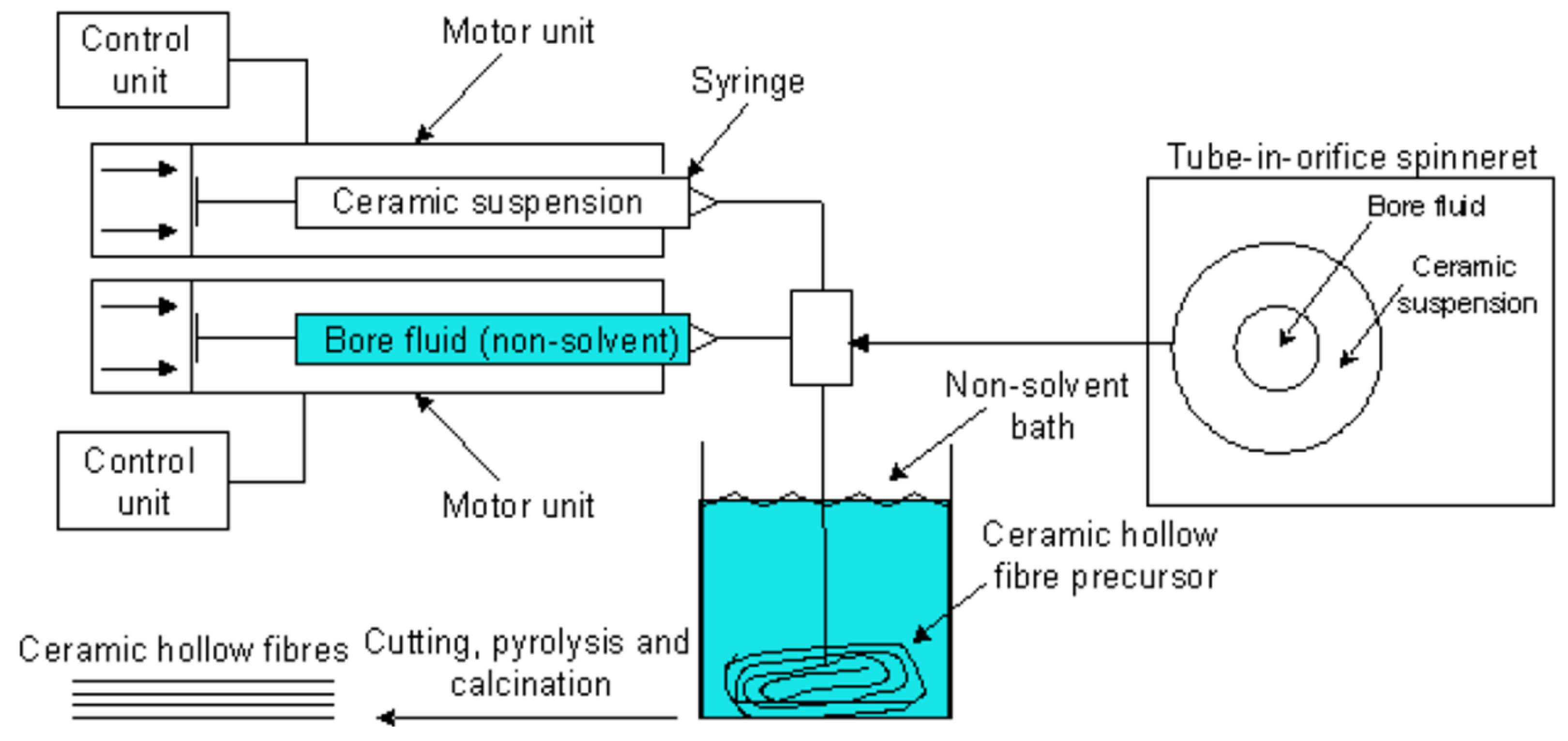
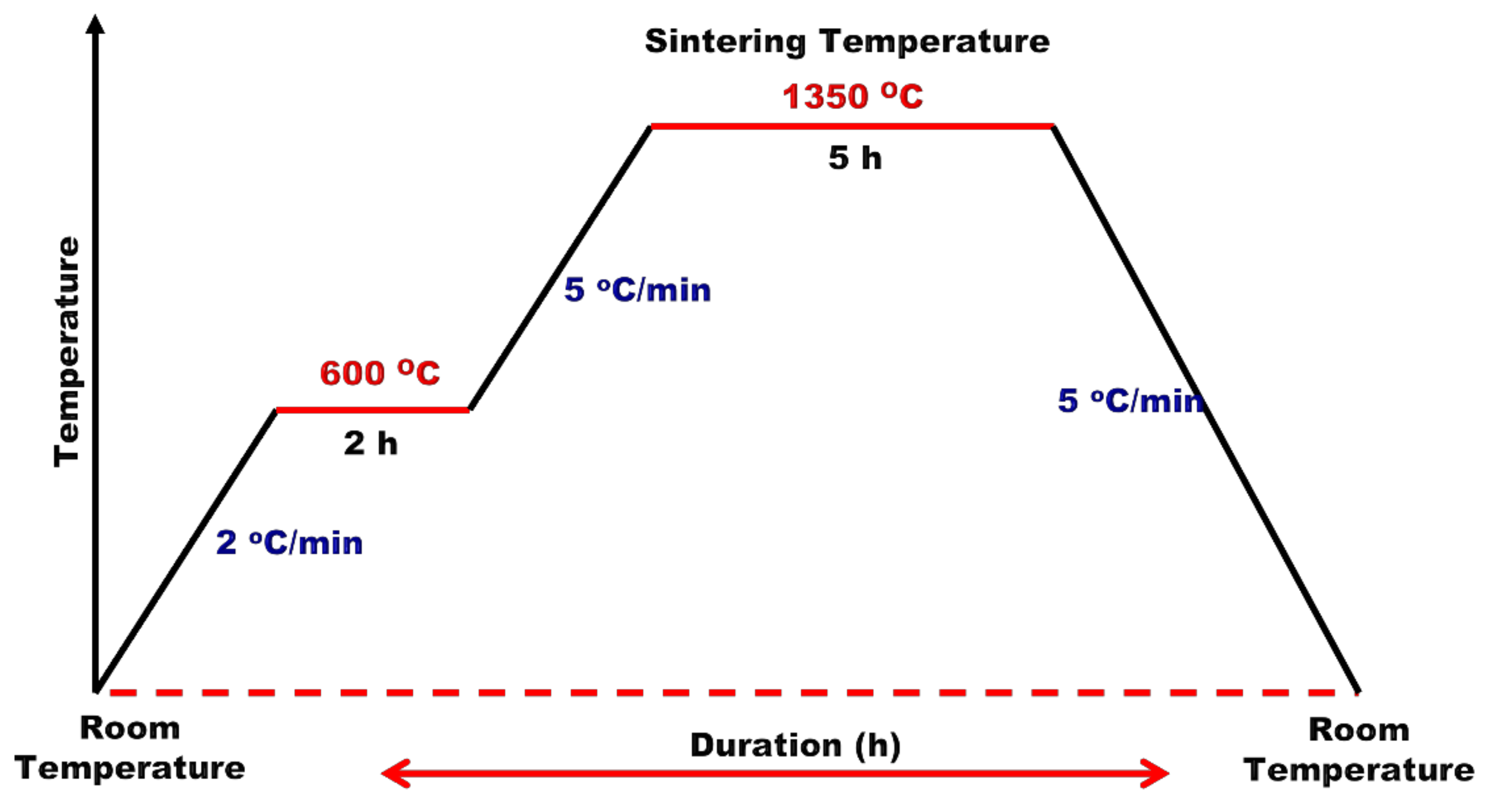
2. Experimental Methodology

The well-known method of phase-inversion coupled with sintering was employed to create the ceramic membrane in this study [30]. Kaolin was first dried in an oven at 80 °C for 24 h. Following that, 1 g of Arlacel P135 gel was dissolved in N-2-methyl-2-pyrrolidone (NMP). This solution was then poured into a ceramic dish with 25 g of ceramic clay powder. The blend then underwent a ball milling process for 48 h using an NQM-2 planetary mill. Afterward, a binder, specifically polyethersulfone (PESF), was incorporated into the mixture and it was milled for an additional 48 h. The homogenized dope suspension was degassed before extrusion by a vacuum pump for 10 min. The degassed dope suspension was then extruded in a single layer spinneret under the flow rate and an extrusion temperature of 10 mL/min and 25 °C, respectively. Distilled water was used as bore fluid and pumped using a syringe pump. Afterwards, the kaolin ceramic hollow fiber membranes were collected and immersed in water for 24 h. In the end, the membranes were washed with water and allowed to dry at ambient temperature for a period of two to three days. Figure 1 depicts the diagram outlining the process of creating the hollow fiber membrane. In the spinneret-based process, the following parameters and values are employed: a spinneret diameter of 1.2; internal and external diameters of 2.8 mm and 10 mm, respectively; a dope extrusion rate of 10 mL/min; an air gap of 5 cm; a bore fluid injection rate of 10 mL/min; and the use of tap water as both an internal and external coagulant. The spinning and external temperatures are maintained at 25 °C. These specific settings constitute the operational conditions for the process, which is characterized by its precise control of variables to achieve the desired outcomes.

The fabricated precursor membrane was cured at 1350 °C using a tubular furnace (XY-1700 MAGNA). The curing began at room temperature, extending for 2 h at a rate of 2 °C/min until 600 °C was achieved. Subsequently, the temperature was raised to 1350 °C at a pace of 5 °C/min and maintained for 5 h. Finally, the temperature was gradually reduced back to ambient levels at 5 °C/min. A diagram showcasing the sintering process of the ceramic membrane can be seen in Figure 2.

A modified Stöber method was adopted for the preparation of the superhydrophobic silica sol-gel solutions [32]. Initially, 0.24 M of tetraethoxysilicate (TEOS) and 4.64 M of ethanol were combined and introduced into a separate solution containing 1.04 M of ammonia, 4.00 M of H2O, and 4.64 M of ethanol. This blend was stirred and underwent a reaction at 60 °C for 90 min to form colloidal silica. Following this, 0.24 M of MTES and 4.64 M of ethanol were incorporated into the previously prepared colloidal silica solutions. An additional 4.64 M of ethanol was added to the mix to instill hydrophobic properties in the silica sol. Then, the solutions were stirred continuously at 60 °C for 19 h and allowed to sit for 3 days for ageing. Finally, the dip-coating method was followed for the preparation of a hydrophobic ceramic membrane.

The filtration experiments were carried out in a custom-designed cross-flow membrane module. The feed flow rate (FF) is varied to understand the influence on flux and oil rejection (L/h). The fouling is majorly influenced by the feed flow rates. The feed flow (FF) can be calculated using Equation (1) below:

$$FF=\frac{V}{t}$$

(1)

In this equation, V represents the feed volume (mL) and t denotes the time (min).

The pH of the feed is another input parameter in tuning the feed characteristics. The feed pH also has an influence on the surface charge of the membrane and it relies on the oil–water separation efficiency.

In oil–water filtration, oil flux (OF) was measured at the time interval of 5 min and calculated according to Equation (2):

$$OF=\frac{V}{A\times t}$$

(2)

In the formula, V represents the oil volume (measured in liters), A stands for the membrane’s surface area (measured in square meters), and t is the duration of filtration (in hours).

The efficiency of separating oil and water, termed oil–water separation efficiency (OSE), is determined by the ratio of oil extracted (m_r) from the initial solution (m_t) by the membrane. It is expressed in the following manner:

$$OSE=\frac{\left(m_r\right)}{m_t}\times 100$$

(3)

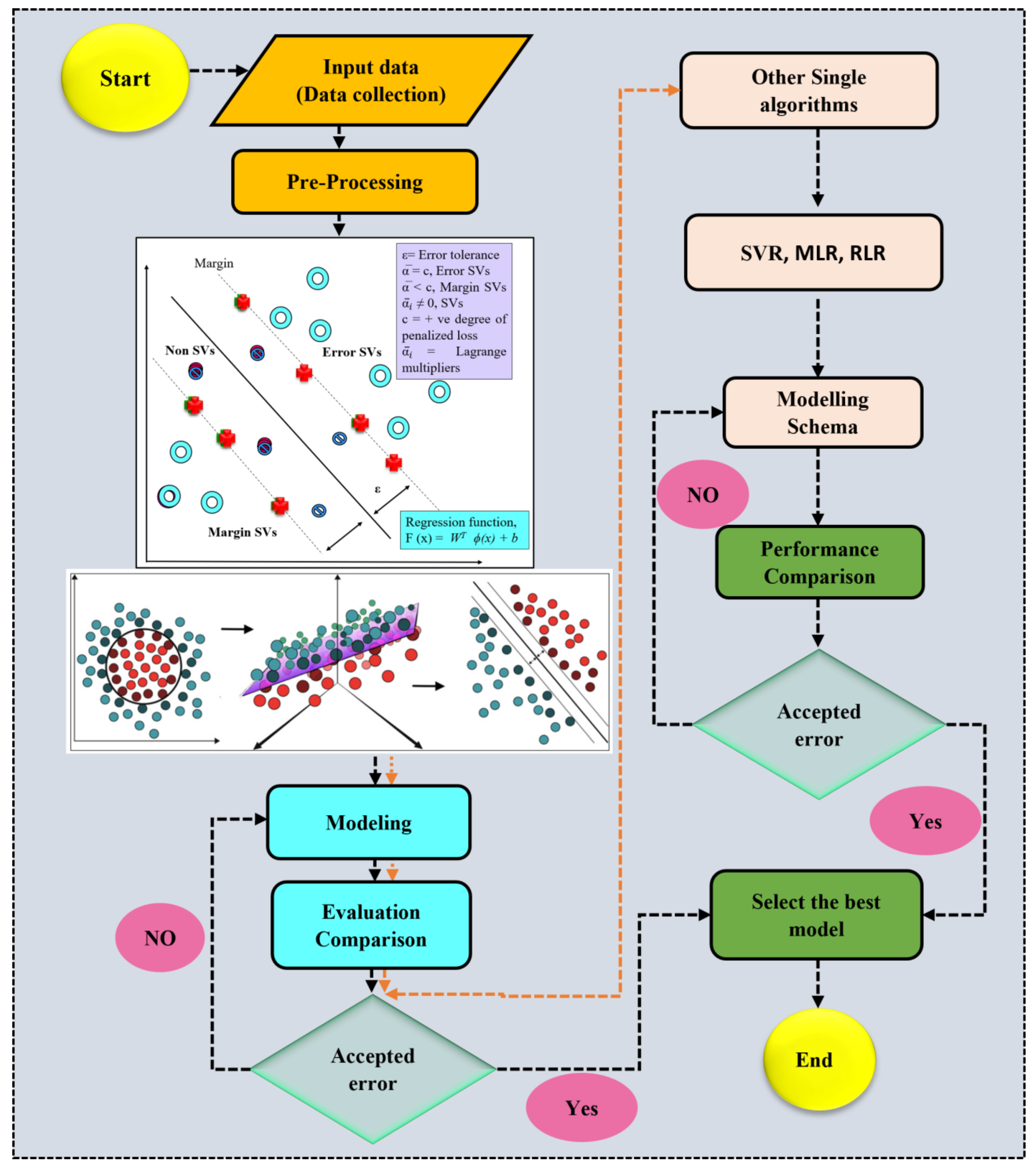
3. Proposed AI Models

The pressing challenge of oil–water separation in wastewater treatment has witnessed a revolutionary improvement with the integration of AI and computational learning. By employing membrane technology, a widely recognized method for separation, AI algorithms analyze vast sets of experimental data to optimize process parameters. The core advantage of AI lies in its ability to predict outcomes with enhanced precision, thereby ensuring the membrane’s maximum efficiency in separating oil from water. Through continuous learning and adaptation, AI models can fine-tune operational conditions, such as pressure, flow rate, and temperature, to achieve optimal separation results. In essence, AI not only streamlines the membrane-based oil–water separation processes but also elevates their efficacy, paving the way for more sustainable wastewater treatment solutions.

The proposed methodology employs a synergistic combination of the SVR, MLR, and RLR approaches to estimate three scenarios, namely, separation efficiency, oil flux, and the combination of the two, in oil–water separation processes through ML [33,34]. This multifaceted approach harnesses the unique strengths of each algorithm. SVR adeptly captures intricate nonlinear correlations, RLR excels at learning intricate patterns, and MLR offers interpretability, allowing a comprehensive understanding of the underlying factors. The models are trained in historical process data, adapting their parameters to difficulties within the dataset, resulting in accurate predictions of the target outputs [35]. To enhance the predictive power and robustness of the models, sensitivity analysis is integrated for feature extractions. This analysis explores the influence of individual input variables on the output predictions, providing insights into the key drivers of the separation process [36,37,38,39]. By leveraging the collective capabilities of SVR, RLR, and MLR, along with the sensitivity analysis, this methodology offers a holistic approach to tackling the challenges of oil–water separation. It contributes to optimized separation processes, leading to increased efficiency and reduced environmental impacts in the oil industry. This integrated framework not only provides accurate predictions but also empowers engineers and researchers to make informed decisions by understanding the sensitivity of the model’s output to various input parameters [40]. For effective ML models in oil–water separation, data were collected from experiments, involving physical and chemical properties of the membrane, as well as operational conditions like pressure and temperature. These data undergo preprocessing, including cleaning and normalization. After identifying the most relevant features through techniques like correlation analysis, the data are divided into training and validation sets. The model is then trained on the chosen features to predict separation efficiency, ensuring its predictions are based on real-world experimental conditions and their intricacies.

3.1. Support Vector Regression

The support vector machine (SVM) has the potent capability to effectively merge classification, regression, prediction, and pattern identification for a specific group of challenges. This is largely because of its innate ability to quickly embrace statistical learning theory and minimize structural risk [41,42]. The potential for the SVM to improve data network performance over traditional AAN is another advantage. Based on their specifications, SVMs can be divided into two groups: nonlinear support vector regression (N-SVR) and linear support vector regression (L-SVR). While the latter is used to analyze nonlinear data and build models, the former is utilized to address immediate technical difficulties like rainfall prediction [43].

The weighting of input variables is dealt with in the first layer while the weighting of output variables is dealt with in the second layer. The general SVR function is provided by Equation (3) for a set of training data $\left\{\left(x_i,d_i\right)\right\}$${}_i^N$ (x_i is the input vector, d_i is the actual value, and N is the total number of data patterns):

$$y=f(x)=w\varphi (x_i)+b$$

(4)

where the nonlinearly transferred feature spaces from the input vector x are denoted by φ(x_i). The regression parameters b and w can be found by providing positive values to the slack parameters ξ and ξ*, minimizing the objective function, as shown in Equation (5):

$$\frac{1}{2}{‖w‖}^2+C\left({\displaystyle {\sum }_i^N({\xi }_i+{\xi }_i^{*})}\right)$$

(5)

$$\mathrm{Subject} \mathrm{to}: \left\{\begin{array}{l}{w}_i\varphi (x_i)+b_i-d_i\le \epsilon +{\xi }_i^{*}\\ d_i-w_i\varphi (x_i)+b_i\le \epsilon +{\xi }_i^{*}\\ {\xi }_i,{\xi }_i^{*}\end{array}\right. i = 1,2,\dots ,\mathrm{N}$$

(6)

where C is the regularized constant and $\frac{1}{2}{‖w‖}^2$ are the weights of the vector norms. The fundamental conceptual model structure of SVR is shown in Figure 3. The vector w in Equation (6) may be calculated after resolving the optimization issue. The Lagrange multipliers’ parameters are represented by α_i and α_i*:

$$w^{*}={\displaystyle {\sum }_{i=1}^N({\alpha }_i-{\alpha }_i^{*})\varphi (x_i)}$$

(7)

As a result, the general form of SVR influences Equation (8):

$$f(x,{\alpha }_i,{\alpha }_i^{*})={\displaystyle {\sum }_{i=1}^N({\alpha }_i-{\alpha }_i^{*})K(x,x_i)+b}$$

(8)

The bias term is b while the kernel function is written as k (x_i, x_j); the Gaussian radial basis function, which can be written as follows, is the most well-liked kernel function:

$$k(x_1,x_2)=\exp (-\gamma {‖x_1-x_2‖}^2)$$

(9)

where γ represents the kernel parameter.

Figure 3. Overall flowchart used in this study.

Figure 3. Overall flowchart used in this study.

3.2. Robust Linear Regression (RLR)

Robust linear regression (RLR) can be categorized into two forms: simple regression, which relates a single predictor to a single variable, and multiple regression, which associates multiple predictors with a single variable. In the context of this research, the analysis utilized multiple regression (also referred to as multilinear regression). It is worth noting that multilinear regression is the most widely used form of linear regression [42,44]. In this analytical approach, every value of an independent variable is mapped to a value of a dependent variable. The linear regression employed in this research is represented by Equation (10).

y = b₀ + b₁ x₁ + b₂ x₂ + … b_i x_i

(10)

Here, x₁ signifies the value of the ith predictor, b₀ represents the regression constant, and bi stands for the coefficient of the ith predictor.

3.3. Multilinear Regression Analysis (MLR)

For building a model where there is a linear relationship between the two parameters, the least squares method is frequently used. Multiple linear regression (MLR) is used to determine the relationship among more than two variables [42,43]. Although multiple linear regression (MLR) is commonly chosen for analysis and model creation because of its ease of use, simple linear regression (SLR) focuses on establishing a connection between two specific variables: the dependent and the independent ones [45]. Below is an example of it in a wider context:

$$y^{\frac{1}{4}}=B_0+B_1{X}_1+B_2{X}_2+B_i{X}_i$$

(11)

B₀ represents the regression constant, X₁ stands for the value of the ith predictor, and B_i is the coefficient of the ith predictor.

3.4. Evaluation Criteria

The effectiveness of any AI-based model for any type of data-driven algorithm can be evaluated using a variety of performance indicators by comparing measured and calculated data [46,47]. Various internal and external validation processes are used to test the models during the verification step [48,49,50]. K-fold cross-validation is one of these techniques that is used in many studies. Similar to this, the computerized model’s substantiation within the scope of its applicability has an appropriate range of accuracy in line with the application that the model is intended for. As a result, the model’s validation techniques should provide the observed levels of agreement between the projected model and the experimental results as well as the model’s prediction accuracy [48,49,50,51,52,53,54]. In this study, external validation was conducted using the k-fold cross-validation method before any modeling was conducted. The authors [42] employed this approach to ascertain the quality of fit gauged using the coefficient of determinacy (R²) and correlation coefficient (CC). Prior to the final development of the model in the simulation phase, a thorough external validation process was thoroughly conducted. This validation procedure relied on the precise 10-fold cross-validation method, strategically designed to fine-tune model performance, improve model integrity, and minimize potential errors in modeling oil flux and separation efficiency. This process partitioned the dataset into ten equal subsets, consecutively utilizing one subset for validation while training the model on the remaining nine, repeating this process ten times to ensure a comprehensive assessment of model generalization. The application of 10-fold cross-validation served a dual purpose: to guard against overfitting, ensuring that models learned meaningful patterns instead of memorizing training data, and to identify potential issues with model robustness and consistency. Consequently, this systematic approach enabled the optimization of model parameters and features in models with superior predictive capabilities, well-suited for real-world applications during the subsequent simulation phase of oil flux and separation efficiency. Additionally, the model’s effectiveness was evaluated using two statistical errors: the root mean square error (RMSE) and the mean square error (MSE). These parameters were assessed using Equations (12)–(15).

The R² (−∞ < R² < 1), CC (−1 < CC < 1), MAE (0 < MAE < ∞), RMSE (0 < RMSE < ∞) are expressed as:

I.

Coefficient of Determinacy

$$\mathrm{R}2=1-\left[\frac{\sum _{i=1}^N(J_{com,i}-J_{pre,i}{)}^2}{\sum _{i=1}^N({J_{com,i}-\overline{J_{com}})}^2}\right]$$

(12)

II.

Correlation Coefficient

$$CC=\frac{\sum _{\mathrm{i}=1}^{\mathrm{N}}\left(J_{com,i}-\overline{J_{com}}\right)\left(J_{pre,i}-\overline{J_{pre}}\right)}{\sqrt{\sum _{\mathrm{i}=1}^{\mathrm{N}}({J_{com,i}-\overline{J_{com}})}^2\sum _{\mathrm{i}=1}^{\mathrm{N}}({J_{pre,i}-\overline{J_{pre}})}^2}}$$

(13)

III.

Mean Square Error

$$MSE=\frac{1}{N} {\sum }_{i=1}^N(J_{com,i}-J_{pre,i}{)}^2$$

(14)

IV.

Root Mean Square Error

$$RMSE=\sqrt{\frac{1}{N} {\sum }_{i=1}^N(J_{com,i}-J_{pre,i}{)}^2}$$

(15)

where J stands for oil flux and $J_{pre,i}$, $J_{com,i}$, $\overline{J_{pre}},$ and $\overline{J_{com}}$ i are the expected and computed values with their corresponding averages for N data points. The best R² and CC and lowest MSE and RMSE proposed models were also put forth for better prediction within the research domain.

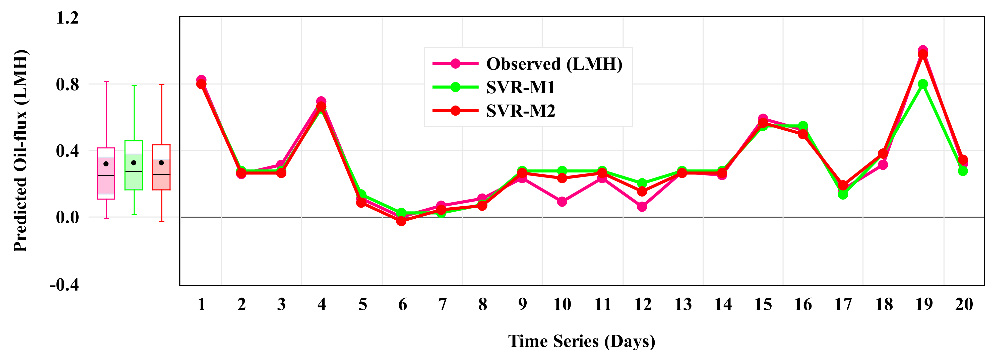
4. Results of AI-Based Models

For model development and coding structure, MATLAB 2022b was used while the other simulation was conducted using EViews-10 software. The graphical analysis was conducted using Origin Pro, Microsoft Excel, and R software. The SVR, RLR, and MLR models were individually employed to prognosticate the separation efficiency and oil flux. The performance potency of each model was appraised employing statistical indicators, namely, R², MSE, root MSE (RMSE), and R.

Table 1. Performance evaluation of SVR, RLR, and MLR in predicting oil flux, separation efficiency, and both in the training phase.

Model	Training Phase (Oil Flux)
	R2	MSE	RMSE	R
SVR-M1	0.9055	0.0049	0.0699	0.9516
SVR-M2	0.9477	0.0027	0.052	0.9735
RLR-M1	0.8151	0.0096	0.0978	0.9029
RLR-M2	0.7889	0.0109	0.1045	0.8882
MLR-M1	0.7936	0.0107	0.1033	0.8908
MLR-M2	0.8369	0.0084	0.0919	0.9148
	Training Phase (S.E)
	R2	MSE	RMSE	R
SVR-M1	0.9781	0.002	0.0444	0.989
SVR-M2	0.9891	0.001	0.0313	0.9946
RLR-M1	0.9752	0.0022	0.0474	0.9875
RLR-M2	0.9777	0.002	0.0449	0.9888
MLR-M1	0.976	0.0022	0.0466	0.9879
MLR-M2	0.9808	0.0017	0.0416	0.9904
	Training Phase (Oil Flux + S.E)
	R2	MSE	RMSE	R
SVR-M1	0.6398	0.0194	0.1394	0.7999
SVR-M2	0.6831	0.0171	0.1308	0.8265
RLR-M1	0.6459	0.0191	0.1382	0.8037
RLR-M2	0.6591	0.0184	0.1356	0.8119
MLR-M1	0.928	0.0039	0.0623	0.9633
MLR-M2	0.9496	0.0027	0.0521	0.9745

and

Table 2. Performance evaluation of SVR, RLR, and MLR in predicting oil flux, separation efficiency, and both in the testing phase.

Model	Testing Phase (Oil Flux)
	R2	MSE	RMSE	R
SVR-M1	0.8859	0.0083	0.0908	0.9412
SVR-M2	0.9847	0.0011	0.0333	0.9923
RLR-M1	0.8943	0.0018	0.0427	0.9457
RLR-M2	0.8683	0.0095	0.0976	0.9318
MLR-M1	0.7931	0.015	0.1223	0.8906
MLR-M2	0.8427	0.0114	0.1067	0.918
	Testing Phase (S.E)
	R2	MSE	RMSE	R
SVR-M1	0.9807	0.0028	0.0526	0.9903
SVR-M2	0.9945	0.0008	0.0282	0.9972
RLR-M1	0.9823	0.0025	0.0505	0.9911
RLR-M2	0.9892	0.0016	0.0394	0.9946
MLR-M1	0.9815	0.0027	0.0516	0.9907
MLR-M2	0.9885	0.0016	0.0406	0.9942
	Testing Phase (Oil Flux + SE)
	R2	MSE	RMSE	R
SVR-M1	0.7809	0.0194	0.1394	0.8837
SVR-M2	0.7856	0.019	0.1378	0.8864
RLR-M1	0.7504	0.0221	0.1487	0.8663
RLR-M2	0.7653	0.0208	0.1442	0.8748
MLR-M1	0.9266	0.0065	0.0807	0.9626
MLR-M2	0.9504	0.0044	0.0663	0.9749

show the computed results for these statistical indicators of training and testing datasets. Additionally, this table shows the multistate performance of the model depending on various input variables. The outcomes indicated that the various predictive modeling strategies had varying degrees of accuracy. Furthermore, SVR-M2 was the superior prediction accuracy for both the training (R² = 0.9477, R = 0.9735, RSME = 0.0520, MSE = 0.0027) and testing phases (R² = 0.9847, R = 0.9923, RMSE = 0.0333, MSE = 0.0011). The worst performing regression method for the prediction of oil flux was MLR-M1, with the computed values of the indicators as training (R² = 0.7936, MSE = 0.0107, RMSE = 0.01033, R = 0.8908) and testing (R² = 0.7931, MSE = 0.0150, RMSE = 0.1223, R = 0.8906). Similarly, for the separation efficiency, SVR-M2 was superior to other modeling techniques with training stage training (R² = 0.9891, MSE = 0.0010, RSME = 0.0313, R = 0.9946) and the testing phase (R² = 0.9945, MSE = 0.0008, RMSE = 0.0282, R = 0.9972); whereas, MLR-M1 had the worst performance with training (R² = 0.9760, MSE = 0.0022, RMSE = 0.0466, R = 0.9879) and testing (R = 0.9815, MSE = 0.0027, RMSE = 0.0516, R = 0.9907). When both responses were simultaneously modeled using the different studied modeling techniques, it was observed that, for training and testing phases, MLR-1 and MLR-2 outdo other techniques in adequately predicting the combination of the responses. This is attributed to the high values of R and R² and low values of MSE and RMSE (Table 1 and Table 2). It was also observed that MLR-2 faintly outdid MLR-1 in terms of these statistical indicators. It is important to note that SVR-M2 is superior to other modelling techniques; this can be attributed to several factors. SVR excels in capturing nonlinear relationships within data, making it effective for modeling complex patterns. It also demonstrates robustness by being less sensitive to outliers, thus accommodating noisy datasets. SVR’s flexibility, enabled by customizable kernel functions, ensures adaptability to diverse data structures and its propensity for generalization aids in reliable predictions for unseen data. Moreover, SVR handles high-dimensional data efficiently and can be fine-tuned through parameter optimization, enhancing its predictive accuracy. The choice of SVR-M2 as superior to other techniques likely depends on the specific dataset, modelling objectives, and performance metrics in the given context.

Figure 4 shows the observed and predicted values of oil flux against the time. It is obvious that the curves for the observed and predicted values for SVR-M2, RLR-M2, and MLR-M2 were nearly stacked on one another while those of the SVR-M2, RLR-M2, and MLR-M2 varied greatly. The same observation was seen for separation efficiency (Figure 5). When the combination of separation efficiency and oil flux is considered, the regression models for MLR-M1 and MLR-M2 had observed and predicted value curves seeming to be almost superimposed (Figure 6). In contrast, the predicted values of other models deviate from the experimental values. This result is in line with what was tabulated in Table 1. Moreover, another visual means of understanding the effectiveness of the different investigated regression models on the prediction of separation efficiency and oil flux is the use of correspondence plots, as illustrated in Figure 7a–f, Figure 8a–f and Figure 9a–f. The correspondence figure makes it clear that the SVR-M2, RLR-M2, and MLR-M2 model outperforms the SVR-M1, RLR-M1, and MLR-M1 models in terms of accuracy. This correspondence plots for the combination of separation efficiency and oil flux when the MRL-M1 and MLR-M2 models were employed. Figure 9e,f demonstrate a strong relationship between the predicted and experimental values, with the data closely following the regression trendline. Efficient oil–water separation is essential for environmental protection and sustainable development. Oil spills harm ecosystems, suffocate marine life, and disrupt oxygen balance in waters. Beyond ecological damage, oil-contaminated water jeopardizes human health, causing ailments and affecting water quality for consumption and agriculture. Economically, oil spills strain fisheries and tourism and necessitate costly clean-ups. Moreover, as industries aim for sustainability, reducing waste and pollution through effective oil–water separation is crucial, exemplified by its importance in the petroleum industry for cleaner extractions. In essence, research in this domain is vital, addressing immediate environmental challenges and promoting a sustainable future.

The bar chart for the computed normalized MSE and RMSE values of the training and testing phases for oil flux and separation efficiency are displayed in Figure 10a–d. The results obtained from these charts validate the results shown in Table 1 where the SVR-M2 regression model had the lowest normalized MSE and RMSE when oil flux (Figure 10a,b) and separation efficiency (Figure 10c,d) were separately used as the output variables. When the combination of the output variables (separation efficiency + oil flux) is considered, for the training and testing phase, the computed normalized MSE and RMSE for the models MLR-M1 and MLR-M2 had the lowest values of this error measurement, as shown in Figure 11a,b. It can be concluded that this research contributes significantly to sustainable development goals (SDGs), for instance, SDG 6, which is focused on guaranteeing access to and the sustainable management of water and sanitation for everyone. By enhancing membrane separation efficiency and oil flux, the methodology addresses wastewater treatment, mitigating water pollution and improving water quality, thus supporting the goal of safe and accessible water resources. In addition, the research directly relates to SDG 12 by promoting responsible consumption and production. By enhancing the efficiency of wastewater treatment, the methodology contributes to minimizing the environmental impact of industries, striving for sustainable production patterns, and reducing the release of harmful substances into the ecosystem.

5. Conclusions

The SVR, RLR, and MLR models were studied to predict the separation efficiency and oil flux. The findings showed that all of the AI models, including SVR, RLR, and MLR, performed excellently across all combinations. SVR-M2 showed to be the most effective simulation tool for oil flux in terms of utilized statistical criteria for both the training (R² = 0.9477, MSE = 0.0027, RSME = 0.0520, R = 0.9735) and testing phases (R² = 0.9847, MSE = 0.0011, RMSE = 0.0333, R = 0.9923) while the worst performing regression method for the prediction of oil flux was MLR-M1 with computed values of the indicators of training (R² = 0.7936, MSE = 0.0107, RMSE = 0.01033, R = 0.8908) and testing (R² = 0.7931, MSE = 0.0150, RMSE = 0.1223, R = 0.8906). Similarly, for the separation efficiency, SVR-M2 was superior to other modeling techniques with training stage training (R² = 0.9891, MSE = 0.0010, RSME = 0.0313, R = 0.9946) and the testing phase (R² = 0.9945, MSE = 0.0008, RMSE = 0.0282, R = 0.9972); whereas, MLR-M1 had the worst performance with training (R² = 0.9760, MSE = 0.0022, RMSE = 0.0466, R = 0.9879) and testing (R = 0.9815, MSE = 0.0027, RMSE = 0.0516, R = 0.9907). When both responses are simultaneously modeled using the different studied modeling techniques, in the training and testing phases, MLR-1 and MLR-2 outdo other techniques in adequately predicting the combination of the responses corresponding to a value of R² higher than 0.9266. MLR-2 faintly outdid MLR-1 in terms of these statistical indicators. This shows that the SVR, RLR, and MLR techniques are promising tools in the prediction of both oil flux and separation efficiency. The results also suggested that hybrid models, emerging algorithms, and optimization methods can be used to enhance filtration performance. The successful integration of AI with membrane-based oil–water separation promises enhanced operational efficiency, cost savings, and superior environmental protection for industries. By optimizing separation processes, industries can achieve faster, more cost-effective results while minimizing environmental impacts. Future research and applications may focus on expanding datasets, refining AI models, real-time monitoring, and tailoring solutions to specific industry needs. Such advancements, combined with the IoT and collaborative efforts, position AI-driven oil–water separation as a pivotal solution for sustainable industrial practices and environmental conservation.

References

1. Gupta, R.K.; Dunderdale, G.J.; England, M.W.; Hozumi, A. Oil/water separation techniques: A review of recent progresses and future directions. J. Mater. Chem. A 2017, 5, 16025–16058. [Google Scholar] [CrossRef]
2. Sabir, S. Approach of cost-effective adsorbents for oil removal from oily water. Crit. Rev. Environ. Sci. Technol. 2015, 45, 1916–1945. [Google Scholar] [CrossRef]
3. Yu, L.; Han, M.; He, F. A review of treating oily wastewater. Arab. J. Chem. 2017, 10, S1913–S1922. [Google Scholar] [CrossRef]
4. Zhang, H.; Bukosky, S.C.; Ristenpart, W.D. Low-Voltage Electrical Demulsification of Oily Wastewater. Ind. Eng. Chem. Res. 2018, 57, 8341–8347. [Google Scholar] [CrossRef]
5. Li, Y. Pretreatment of Oilfield Produced Water Using Ionic Liquids for Dissolved Air. Ph.D. Thesis, Faculty of Graduate Studies and Research, University of Regina, Regina, SK, Canada, 2017. [Google Scholar]
6. Labhasetwar, P.K.; Yadav, A. Membrane Based Point-of-Use Drinking Water Treatment Systems; IWA Publishing: London, UK, 2023; ISBN 9781789062724. [Google Scholar]
7. Usman, J.; Othman, M.H.D.; Ismail, A.F.; Rahman, M.A.; Jaafar, J.; Raji, Y.O.; El Badawy, T.H.; Gbadamosi, A.O.; Kurniawan, T.A. Impact of organosilanes modified superhydrophobic-superoleophilic kaolin ceramic membrane on efficiency of oil recovery from produced water. J. Chem. Technol. Biotechnol. 2020, 95, 3300–3315. [Google Scholar] [CrossRef]
8. Usman, J.; Hafiz, M.; Othman, D.; Fauzi, A.; Rahman, M.A.; Jaafar, J.; Olabode, Y.; Gbadamosi, A.O.; Hassan, T.; Badawy, E. An overview of superhydrophobic ceramic membrane surface modification for oil-water separation. J. Mater. Res. Technol. 2021, 12, 643–667. [Google Scholar] [CrossRef]
9. Liu, J.; Li, P.; Chen, L.; Feng, Y.; He, W.; Lv, X. Modified superhydrophilic and underwater superoleophobic PVDF membrane with ultralow oil-adhesion for highly efficient oil/water emulsion separation. Mater. Lett. 2016, 185, 169–172. [Google Scholar] [CrossRef]
10. Wu, H.; Shi, J.; Ning, X.; Long, Y.-Z.; Zheng, J. The High Flux of Superhydrophilic-Superhydrophobic Janus Membrane of cPVA-PVDF/PMMA/GO by Layer-by-Layer Electrospinning for High Efficiency Oil-Water Separation. Polymers 2022, 14, 621. [Google Scholar] [CrossRef] [PubMed]
11. Lu, J.; Yu, Y.; Zhou, J.; Song, L.; Hu, X.; Larbot, A. FAS grafted superhydrophobic ceramic membrane. Appl. Surf. Sci. 2009, 255, 9092–9099. [Google Scholar] [CrossRef]
12. Ibrahim, M.; Salami, B.A.; Amer Algaifi, H.; Kalimur Rahman, M.; Nasir, M.; Ewebajo, A.O. Assessment of acid resistance of natural pozzolan-based alkali-activated concrete: Experimental and optimization modelling. Constr. Build. Mater. 2021, 304, 124657. [Google Scholar] [CrossRef]
13. Algaifi, H.A.; Khan, M.I.; Shahidan, S.; Fares, G.; Abbas, Y.M.; Huseien, G.F.; Salami, B.A.; Alabduljabbar, H. Strength and acid resistance of ceramic-based self-compacting alkali-activated concrete: Optimizing and predicting assessment. Materials 2021, 14, 6208. [Google Scholar] [CrossRef]
14. Usman, A.G.; IŞIK, S.; Abba, S.I. Qualitative prediction of Thymoquinone in the high-performance liquid chromatography optimization method development using artificial intelligence models coupled with ensemble machine learning. Sep. Sci. Plus 2022, 5, 579–587. [Google Scholar] [CrossRef]
15. Zobel, C.W.; Cook, D.F. Evaluation of neural network variable influence measures for process control. Eng. Appl. Artif. Intell. 2011, 24, 803–812. [Google Scholar] [CrossRef]
16. Okpalaeke, K.E.; Ibrahim, T.H.; Latinwo, L.M.; Betiku, E. Mathematical Modeling and Optimization Studies by Artificial Neural Network, Genetic Algorithm and Response Surface Methodology: A Case of Ferric Sulfate–Catalyzed Esterification of Neem (Azadirachta indica) Seed Oil. Front. Energy Res. 2020, 8, 614621. [Google Scholar] [CrossRef]
17. Betiku, E.; Ajala, S.O. Modeling and optimization of Thevetia peruviana (yellow oleander) oil biodiesel synthesis via Musa paradisiacal (plantain) peels as heterogeneous base catalyst: A case of artificial neural network vs. response surface methodology. Ind. Crops Prod. 2014, 53, 314–322. [Google Scholar] [CrossRef]
18. Khatti, T.; Naderi-Manesh, H.; Kalantar, S.M. Application of ANN and RSM techniques for modeling electrospinning process of polycaprolactone. Neural Comput. Appl. 2019, 31, 239–248. [Google Scholar] [CrossRef]
19. Pham, Q.B.; Sammen, S.S.; Abba, S.I.; Mohammadi, B.; Shahid, S.; Abdulkadir, R.A. A new hybrid model based on relevance vector machine with flower pollination algorithm for phycocyanin pigment concentration estimation. Environ. Sci. Pollut. Res. 2021, 28, 32564–32579. [Google Scholar] [CrossRef] [PubMed]
20. Sarve, A.; Sonawane, S.S.; Varma, M.N. Ultrasound assisted biodiesel production from sesame (Sesamum indicum L.) oil using barium hydroxide as a heterogeneous catalyst: Comparative assessment of prediction abilities between response surface methodology (RSM) and artificial neural network (ANN). Ultrason. Sonochem. 2015, 26, 218–228. [Google Scholar] [CrossRef] [PubMed]
21. Ma, L.; Lv, E.; Du, L.; Lu, J.; Ding, J. Statistical modeling/optimization and process intensification of microwave-assisted acidified oil esterification. Energy Convers. Manag. 2016, 122, 411–418. [Google Scholar] [CrossRef]
22. Usman, A.G.; IŞik, S.; Abba, S.I.; MerİÇlİ, F. Artificial intelligence-based models for the qualitative and quantitative prediction of a phytochemical compound using HPLC method. Turk. J. Chem. 2020, 44, 1339–1351. [Google Scholar] [CrossRef] [PubMed]
23. Nandi, B.K.; Moparthi, A.; Uppaluri, R.; Purkait, M.K. Treatment of oily wastewater using low cost ceramic membrane: Comparative assessment of pore blocking and artificial neural network models. Chem. Eng. Res. Des. 2010, 88, 881–892. [Google Scholar] [CrossRef]
24. Chen, P.-C.; Xu, Z.-K. Mineral-Coated Polymer Membranes with Superhydrophilicity and Underwater Superoleophobicity for Effective Oil/Water Separation. Sci. Rep. 2013, 3, 2776. [Google Scholar] [CrossRef]
25. Rahimzadeh, A.; Ashtiani, F.Z.; Okhovat, A. Application of adaptive neuro-fuzzy inference system as a reliable approach for prediction of oily wastewater microfiltration permeate volume. J. Environ. Chem. Eng. 2016, 4, 576–584. [Google Scholar] [CrossRef]
26. Ma, W.; Samal, S.K.; Liu, Z.; Xiong, R.; De Smedt, S.C.; Bhushan, B.; Zhang, Q.; Huang, C. Dual pH- and ammonia-vapor-responsive electrospun nanofibrous membranes for oil-water separations. J. Memb. Sci. 2017, 537, 128–139. [Google Scholar] [CrossRef]
27. Zhu, Y.; Xie, W.; Zhang, F.; Xing, T.; Jin, J. Superhydrophilic In-Situ-Cross-Linked Zwitterionic Polyelectrolyte/PVDF-Blend Membrane for Highly Efficient Oil/Water Emulsion Separation. ACS Appl. Mater. Interfaces 2017, 9, 9603–9613. [Google Scholar] [CrossRef] [PubMed]
28. Kang, H.; Cheng, Z.; Lai, H.; Ma, H.; Liu, Y.; Mai, X.; Wang, Y.; Shao, Q.; Xiang, L.; Guo, X.; et al. Superlyophobic anti-corrosive and self-cleaning titania robust mesh membrane with enhanced oil/water separation. Sep. Purif. Technol. 2018, 201, 193–204. [Google Scholar] [CrossRef]
29. Ismail, N.H.; Salleh, W.N.W.; Ismail, A.F.; Hasbullah, H.; Yusof, N.; Aziz, F.; Jaafar, J. Hydrophilic polymer-based membrane for oily wastewater treatment: A review. Sep. Purif. Technol. 2020, 233, 116007. [Google Scholar] [CrossRef]
30. Usman, J.; Salami, B.A.; Gbadamosi, A.; Adamu, H.; GarbaUsman, A.; Benaafi, M.; Abba, S.I.; Dzarfan Othman, M.H.; Aljundi, I.H. Intelligent optimization for modelling superhydrophobic ceramic membrane oil flux and oil-water separation efficiency: Evidence from wastewater treatment and experimental laboratory. Chemosphere 2023, 331, 138726. [Google Scholar] [CrossRef] [PubMed]
31. Li, H.; Mu, P.; Li, J.; Wang, Q. Inverse desert beetle-like ZIF-8/PAN composite nanofibrous membrane for highly efficient separation of oil-in-water emulsions. J. Mater. Chem. A 2021, 9, 4167–4175. [Google Scholar] [CrossRef]
32. Stöber, W.; Fink, A.; Bohn, E. Controlled Growth of Monodisperse Silica Spheres in the Micron Size Range. J. Colloid Interface Sci. 1968, 69, 62–69. [Google Scholar] [CrossRef]
33. Alhaji, U.; Chinemezu, E.; Isah, S. Bioresource Technology Reports Machine learning models for biomass energy content prediction: A correlation-based optimal feature selection approach. Bioresour. Technol. Rep. 2022, 19, 101167. [Google Scholar] [CrossRef]
34. Alhaji, U.; Chinemezu, E.; Nwachukwu, J.; Isah, S. Prediction of energy content of biomass based on hybrid machine learning ensemble algorithm. Energy Nexus 2022, 8, 100157. [Google Scholar] [CrossRef]
35. Baig, N.; Usman, J.; Abba, S.I.; Benaafi, M.; Aljundi, I.H. Fractionation of dyes/salts using loose nanofiltration membranes: Insight from machine learning prediction. J. Clean. Prod. 2023, 418, 138193. [Google Scholar] [CrossRef]
36. Abdullahi, H.U.; Usman, A.G.; Abba, S.I.; Abdullahi, H.U. Modelling the Absorbance of a Bioactive Compound in HPLC Method using Artificial Neural Network and Multilinear Regression Methods. Dutse J. Pure Appl. Sci. 2020, 6, 362–371. [Google Scholar]
37. Usman, A.G.; Işik, S.; Abba, S.I. A Novel Multi-model Data-Driven Ensemble Technique for the Prediction of Retention Factor in HPLC Method Development. Chromatographia 2020, 83, 933–945. [Google Scholar] [CrossRef]
38. Benaafi, M.; Tawabini, B.; Abba, S.I.; Humphrey, J.D.; Al-Areeq, A.M.; Alhulaibi, S.A.; Usman, A.G.; Aljundi, I.H. Integrated Hydrogeological, Hydrochemical, and Isotopic Assessment of Seawater Intrusion into Coastal Aquifers in Al-Qatif Area, Eastern Saudi Arabia. Molecules 2022, 27, 6841. [Google Scholar] [CrossRef] [PubMed]
39. Abba, S.I.; Pham, Q.B.; Usman, A.G.; Linh, N.T.T.; Aliyu, D.S.; Nguyen, Q.; Bach, Q.V. Emerging evolutionary algorithm integrated with kernel principal component analysis for modeling the performance of a water treatment plant. J. Water Process Eng. 2020, 33, 101081. [Google Scholar] [CrossRef]
40. Abubakar, A.; Jibril, M.M.; Almeida, C.F.M.; Gemignani, M.; Yahya, M.N.; Abba, S.I. A Novel Hybrid Optimization Approach for Fault Detection in Photovoltaic Arrays and Inverters Using AI and Statistical Learning Techniques: A Focus on Sustainable Environment. Processes 2023, 11, 2549. [Google Scholar] [CrossRef]
41. Adamu, M.; Haruna, S.I.; Malami, S.I.; Ibrahim, M.N.; Abba, S.I.; Ibrahim, Y.E. Prediction of compressive strength of concrete incorporated with jujube seed as partial replacement of coarse aggregate: A feasibility of Hammerstein–Wiener model versus support vector machine. Model. Earth Syst. Environ. 2021, 8, 3435–3445. [Google Scholar] [CrossRef]
42. Malami, S.I.; Anwar, F.H.; Abdulrahman, S.; Haruna, S.I.; Ali, S.I.A.; Abba, S.I. Implementation of hybrid neuro-fuzzy and self-turning predictive model for the prediction of concrete carbonation depth: A soft computing technique. Results Eng. 2021, 10, 100228. [Google Scholar] [CrossRef]
43. Nourani, V.; Elkiran, G.; Abba, S.I. Wastewater treatment plant performance analysis using artificial intelligence—An ensemble approach. Water Sci. Technol. 2018, 78, 2064–2076. [Google Scholar] [CrossRef]
44. Tahsin, A.; Abdullahi, J.; Rotimi, A.; Anwar, F.H.; Malami, S.I.; Abba, S.I. Multi-state comparison of machine learning techniques in modelling reference evapotranspiration: A case study of Northeastern Nigeria. In Proceedings of the 2021 1st International Conference on Multidisciplinary Engineering and Applied Science (ICMEAS), Abuja, Nigeria, 15–16 July 2021; pp. 1–6. [Google Scholar] [CrossRef]
45. Kemper, T.; Sommer, S. Estimate of heavy metal contamination in soils after a mining accident using reflectance spectroscopy. Environ. Sci. Technol. 2002, 36, 2742–2747. [Google Scholar] [CrossRef] [PubMed]
46. Wiangkham, A.; Ariyarit, A.; Aengchuan, P. Prediction of the influence of loading rate and sugarcane leaves concentration on fracture toughness of sugarcane leaves and epoxy composite using artificial intelligence. Theor. Appl. Fract. Mech. 2022, 117, 103188. [Google Scholar] [CrossRef]
47. Doulati Ardejanii, F.; Rooki, R.; Jodieri Shokri, B.; Eslam Kish, T.; Aryafar, A.; Tourani, P. Prediction of Rare Earth Elements in Neutral Alkaline Mine Drainage from Razi Coal Mine, Golestan Province, Northeast Iran, Using General Regression Neural Network. J. Environ. Eng. 2013, 139, 896–907. [Google Scholar] [CrossRef]
48. Pham, Q.B.; Abba, S.I.; Usman, A.G.; Thi, N.; Linh, T. Potential of Hybrid Data-Intelligence Algorithms for Multi-Station Modelling of Rainfall. Water Resour. Manag. 2019, 33, 5067–5087. [Google Scholar] [CrossRef]
49. Abba, S.I.; Linh, N.T.T.; Abdullahi, J.; Ali, S.I.A.; Pham, Q.B.; Abdulkadir, R.A.; Costache, R.; Nam, V.T.; Anh, D.T. Hybrid machine learning ensemble techniques for modeling dissolved oxygen concentration. IEEE Access 2020, 8, 157218–157237. [Google Scholar] [CrossRef]
50. Asnake Metekia, W.; Garba Usman, A.; Hatice Ulusoy, B.; Isah Abba, S.; Chirkena Bali, K. Artificial intelligence-based approaches for modeling the effects of spirulina growth mediums on total phenolic compounds. Saudi J. Biol. Sci. 2022, 29, 1111–1117. [Google Scholar] [CrossRef] [PubMed]
51. Elkiran, G.; Nourani, V.; Abba, S.I.; Abdullahi, J. Artificial intelligence-based approaches for multi-station modelling of dissolve oxygen in river. Glob. J. Environ. Sci. Manag. 2018, 4, 439–450. [Google Scholar] [CrossRef]
52. Manzar, M.S.; Benaafi, M.; Costache, R.; Alagha, O.; Mu’azu, N.D.; Zubair, M.; Abdullahi, J.; Abba, S.I. New generation neurocomputing learning coupled with a hybrid neuro-fuzzy model for quantifying water quality index variable: A case study from Saudi Arabia. Ecol. Inform. 2022, 70, 101696. [Google Scholar] [CrossRef]
53. Usman, A.G.; Işik, S.; Abba, S.I.; Meriçli, F. Chemometrics-based models hyphenated with ensemble machine learning for retention time simulation of isoquercitrin in Coriander sativum L. using high-performance liquid chromatography. J. Sep. Sci. 2021, 44, 843–849. [Google Scholar] [CrossRef]
54. Abba, S.I.; Hadi, S.J.; Abdullahi, J. River water modelling prediction using multi-linear regression, artificial neural network, and adaptive neuro-fuzzy inference system techniques. Procedia Comput. Sci. 2017, 120, 75–82. [Google Scholar] [CrossRef]
Figure 1. The schematic demonstration of the spinning process of the ceramic membrane fabrication process.
Water 15 03611 g001
Figure 2. Sintering profile of the ceramic membrane.
Water 15 03611 g002
Figure 4. Observed and predicted values of oil flux from the models against the time series.
Water 15 03611 g004aWater 15 03611 g004b
Figure 5. Observed and predicted values of separation efficiency from the models against the time series.
Water 15 03611 g005aWater 15 03611 g005b
Figure 6. Observed and predicted values of separation efficiency and oil flux from the models against the time series.
Water 15 03611 g006
Figure 7. Scatter plots of oil flux for LMH between the observed and predicted values, (a) Normalized predicted SVR-M1(LMH) vs. Normalized observed oil flux (LMH), (b) Normalized predicted SVR-M2(LMH) vs. Normalized observed oil flux (LMH), (c) Normalized predicted RLR-M1(LMH) vs. Normalized observed oil flux (LMH), (d) Normalized predicted RLR-M2(LMH) vs. Normalized observed oil flux (LMH), (e) Normalized predicted MLR-M1(LMH) vs. Normalized observed oil flux (LMH) and (f) Normalized predicted MLR-M2(LMH) vs. Normalized observed oil flux (LMH).
Water 15 03611 g007
Figure 8. Scatter plots of separation efficiency based on observed and predicted values, (a) Normalized predicted SVR-M1(%) vs. Normalized observed separation efficiency (%), (b) Normalized predicted SVR-M2(%) vs. Normalized observed separation efficiency (%), (c) Normalized predicted RLR-M1(%) vs. Normalized observed separation efficiency (%), (d) Normalized predicted RLR-M2(%) vs. Normalized observed separation efficiency (%), (e) Normalized predicted MLR-M1(%) vs. Normalized observed separation efficiency (%) and (f) Normalized predicted MLR-M2(%) vs. Normalized observed separation efficiency (%).
Water 15 03611 g008
Figure 9. Scatter plots of separation efficiency and oil flux (%&LMH), (a) Normalized predicted SVR-M1(%&LMH) vs. Normalized observed separation efficiency and oil flux (%&LMH), (b) Normalized predicted SVR-M2(%&LMH) vs. Normalized observed separation efficiency and oil flux (%&LMH), (c) Normalized predicted RLR-M1(%&LMH) vs. Normalized observed separation efficiency (%&LMH), (d) Normalized predicted RLR-M2(%&LMH) vs. Normalized observed separation efficiency and oil flux (%&LMH), (e) Normalized predicted MLR-M1(%&LMH) vs. Normalized observed separation efficiency and oil flux (%&LMH) and (f) Normalized predicted MLR-M2(%&LMH) vs. Normalized observed separation efficiency and oil flux (%&LMH).
Water 15 03611 g009
Figure 10. Error graph of oil flux (a,b) and separation efficiency (c,d) for comparison, (a) Normalized MSE for oil flux vs. models, (b) Normalized RMSE for oil flux vs. models, (c) Normalized MSE for separation efficiency vs. models, (d) Normalized RMSE for separation efficiency vs. models.
Water 15 03611 g010
Figure 11. Error graph of combined output (oil flux and separation efficiency) for comparison, (a) Normalized MSE for separation efficiency and oil flux vs. models, (b) Normalized RMSE for separation efficiency and oil flux vs. models.
Water 15 03611 g011