A Machine Learning Framework for Enhancing Short-Term Water Demand Forecasting Using Attention-BiLSTM Networks Integrated with XGBoost Residual Correction

Abstract

Accurate short-term water demand forecasting assumes a pivotal role in optimizing water supply control strategies, constituting a cornerstone of effective water management. In recent times, the rise of machine learning technologies has ushered in hybrid models that exhibit superior performance in this domain. Given the intrinsic non-linear fluctuations and variations in short-term water demand sequences, achieving precise forecasts presents a formidable challenge. Against this backdrop, this study introduces an innovative machine learning framework for short-term water demand prediction. The maximal information coefficient (MIC) is employed to select high-quality input features. A deep learning architecture is devised, featuring an Attention-BiLSTM network. This design leverages attention weights and the bidirectional information in historical sequences to highlight influential factors and enhance predictive capabilities. The integration of the XGBoost algorithm as a residual correction module further bolsters the model’s performance by refining predicted results through error simulation. Hyper-parameter configurations are fine-tuned using the Keras Tuner and random parameter search. Through rigorous performance comparison with benchmark models, the superiority and stability of this method are conclusively demonstrated. The attained results unequivocally establish that this approach outperforms other models in terms of predictive accuracy, stability, and generalization capabilities, with MAE, RMSE, MAPE, and NSE values of 544 m³/h, 915 m³/h, 1.00%, and 0.99, respectively. The study reveals that the incorporation of important features selected by the MIC, followed by their integration into the attention mechanism, essentially subjects these features to a secondary filtration. While this enhances model performance, the potential for improvement remains limited. Our proposed forecasting framework offers a fresh perspective and contribution to the short-term water resource scheduling in smart water management systems.

1. Introduction

Due to the rapid pace of urbanization, the establishment of an intelligent water demand forecasting system has emerged as a critical component of smart city development [1]. The accuracy of water demand prediction serves as the fundamental cornerstone for constructing such an intelligent system. This precision enables water utilities to minimize energy consumption costs linked to water pump operations while simultaneously fulfilling user requirements, thereby achieving a balanced equilibrium between water production and consumption [2]. Water demand also assumes a vital role in monitoring efforts, evident in its capacity to detect potential leakage instances when actual demand values significantly deviate from the projected water demand [3]. The topic of water demand forecasting has been a focal point of research since the 1960s [4], encompassing various forecasting timeframes, notably long-term, medium-term, and short-term [5]. Diverse viewpoints from researchers have proposed distinct intervals for short-term horizon forecasting, ranging from minutes and hours to days and weeks [6,7]. From a planning perspective, long-term water demand forecasting may prove to be more effective, as it estimates the water resource requirements for future years or even decades of socio-economic development, providing essential groundwork for the formulation of water security strategies. However, from the standpoint of smart water management construction, short-term water resource prediction serves as the foundation of urban water resource scheduling, contributing to the enhanced optimization of water resource utilization and facilitating daily water resource management [8]. For instance, Liu et al. [9] introduced a daily water demand model for Shenzhen city, which supports the daily scheduling process of water resources, better addressing the water scarcity challenges faced by major urban areas. To ensure clarity, this study adopts the concept of short-term forecasting with a 1 h interval.

Regarding the existing body of literature pertaining to water demand forecasting, approaches for addressing this matter can generally be classified into linear mathematical methods and nonlinear techniques. For example, within the realm of water demand forecasting, the autoregressive integrated moving average (ARIMA) model and the seasonal autoregressive integrated moving average (SARIMA) model have gained widespread acceptance due to their relatively simple interpretability and practical applicability [10,11,12]. Nevertheless, classical statistical models such as ARIMA solely rely on historical data and the assumption of a normal distribution to establish correlations between past and future values [13]. Given the multitude of factors influencing water demand, Wang et al. [14] employed a multivariate linear regression (MLR) technique to accomplish water demand forecasting. However, these linear methodologies may encounter challenges in capturing the intricate nonlinear relationships within demand trends, thereby leading to potentially flawed predictions [10,14].

In the present context, propelled by the rapid advancements in computer technology and data mining, machine learning, falling under the category of nonlinear methodologies, offers the potential for achieving more precise water demand predictions. A plethora of techniques, including artificial neural networks (ANN), support vector regression (SVR), random forest (RF), and gradient boosting machine (GBM), have been proposed and adopted within this domain [15,16]. Numerous studies have underscored the significant improvements brought about by these methods in comparison to conventional linear models. However, it remains a challenge for these methods to fully meet the expected accuracy required for optimal water utilities scheduling [17]. Deep learning, a highly regarded subset of machine learning, has witnessed extensive applications in areas such as face recognition, text classification, and object detection [18,19,20]. Moreover, short-term water demand forecasting has also been benefiting from its capabilities. Guo et al. [7] employed the gated recurrent unit network (GRUN) for short-term water demand forecasting with a 15 min time resolution, demonstrating superior forecasting performance of GRUN over ANN. Zanfei et al. [21] devised an ensemble model comprising the simple recurrent network (SRNN), long short memory network (LSTM), and GRU, which were respectively applied to 1 h and 24 h water demand forecasting. Similarly, Chen et al. [22] introduced an innovative forecasting framework termed Conv1D-GRU, achieving 15 min water consumption forecasts. The Conv1D-GRU model exhibited enhanced accuracy in forecasting and greater adaptability for extracting data features compared to GRUN and ANN. However, it is important to note that recurrent networks such as LSTM and GRU primarily capture forward data patterns, potentially overlooking the influence of backward information on prediction.

In recent years, Bahdanau et al. [23] pioneered the incorporation of the attention mechanism into seq2seq models, revolutionizing the field of deep learning. This mechanism, reminiscent of human visual processing, selectively concentrates on valuable information to enhance prediction accuracy. This technique’s efficacy has been showcased across diverse domains such as electricity load forecasting and traffic flow prediction [24,25]. However, its application in water demand forecasting remains underrepresented in current research. With the deepening research into hybrid models, numerous studies have demonstrated their potential to enhance predictive capabilities. By leveraging the advantages of different model combinations and delving into the uncertainties of internal data features, these models aim to maximize predictive performance. Du et al. [26] introduced the hybrid model KDE-PSO-LSTM, which combines kernel density estimation (KDE) and particle swarm optimization (PSO) algorithms to fit a probability density curve of forecast errors. This approach is used to obtain water demand prediction intervals, thereby quantifying prediction uncertainty. Guo et al. [27] proposed a novel hybrid forecasting model that integrates temporal convolutional neural networks, discrete wavelet transform, and random forests to improve the accuracy and efficiency of water demand forecasting.

After extensive research efforts, it becomes evident that deep learning has made significant strides in the realm of water demand prediction, thereby laying a solid foundation for subsequent investigations. However, there remain certain aspects that merit attention and enhancement. (1) A recurring observation among various researchers is the employment of recurrent neural network structures such as LSTM, which primarily capture forward data trends while neglecting the influence of reverse information on predictions. This limitation may result in an insufficient reflection of the intricate characteristics embedded within water demand series. (2) In the context of current demand estimations, specific historical data points within the sequences could possess higher significance than others. Regrettably, the existing network structures fail to appropriately allocate attention based on the relative importance of these data points, consequently leading to reduced prediction accuracy. (3) An opportunity arises when the pattern of residuals between forecasted values and observed values can be effectively simulated. This simulation has the potential to significantly enhance the overall performance of the models.

The innovation and contribution of this paper lie in introducing an innovative hybrid model within a machine learning framework in response to the issues outlined above. It proposes the integration of a bidirectional long short memory neural network (BiLSTM) with an attention mechanism, giving rise to the coined term “Attention-BiLSTM network”. This architecture is tailored for short-term water demand forecasting. BiLSTM is employed to learn the forward and backward patterns in historical water usage data, and an attention mechanism is introduced to emphasize the influence of key historical sequences. Furthermore, an additional step is incorporated in the form of a residual correction module, leveraging the capabilities of the XGBoost algorithm. This module serves the dual purpose of error prediction and refining the results of the prediction model. This augmentation is specifically designed to bolster the forecasting capacity of the models.

The structure of this study is outlined as follows. Section 2 provides an overview and essential details of the proposed procedure for short-term water demand forecasting. In Section 3, the effectiveness of the Attention-BiLSTM network combined with the XGBoost algorithm for residual correction is tested using real-world data. This includes the Section 3.3, which analyzes the variation of attention mechanism weights with sequence spans, compares the performance of the proposed approach with other benchmark models (including LSTM and BiLSTM), and extracts hidden insights from the evaluation metrics. Finally, Section 4 presents concluding remarks and outlines avenues for future research.

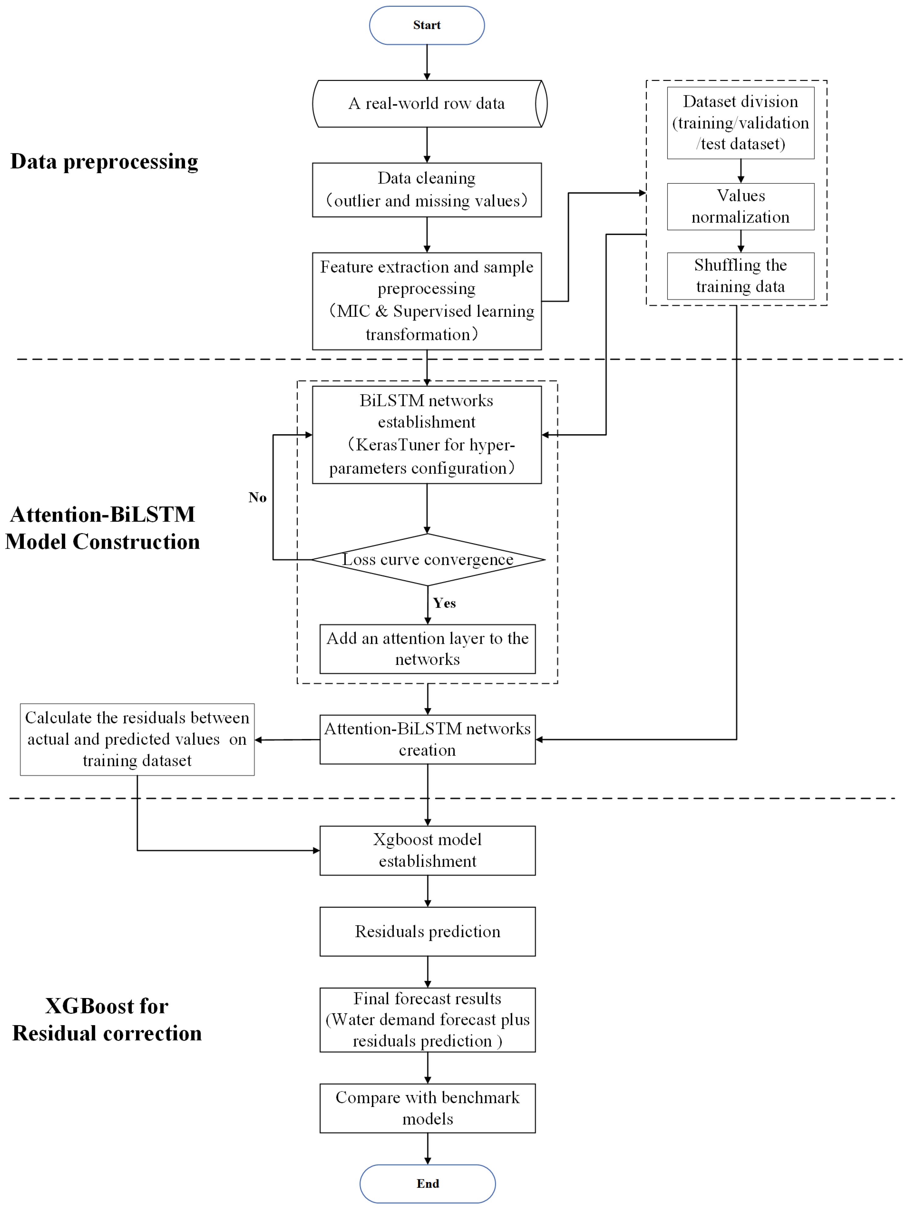
2. Methodology

Figure 1 illustrates the complete water demand forecasting process using the proposed method. Initially, data cleaning was performed on the collected water demand series. The maximum information coefficient (MIC) method was utilized to select highly correlated historical sequence data with the current values. Subsequently, a sliding window scheme was employed to transform the data into a supervised learning problem. The construction of the Attention-BiLSTM networks, coupled with the XGBoost algorithm for the residual correction module, was then presented in detail. Utilizing random parameter search, key parameters for each model were determined, and the predictive performance of the models was observed through convergence curves. Finally, the proposed method was applied to short-term water demand forecasting, and its performance was assessed.

2.1. Maximal Information Coefficient Method

Given the inherent periodicity and trend in water demand, historical water demand data serve as the essential underpinning for forecasting current demand [28]. The MIC method exhibits robustness and low computational complexity in addressing correlation analysis issues [29]. Thus, this study employs the MIC method to scrutinize correlations between different variables and current water demand data, with the objective of acquiring inputs that enhance model quality.

The MIC method is constructed upon the framework of mutual information. It quantifies linear or nonlinear functional connections between random variables through grid-based partitioning, thereby offering a more comprehensive portrayal of non-functional interdependencies among variables [29]. For binary dataset $D\in R^2$, given two variables $X=\left\{x_i,i=1,2,\dots ,n\right\}$, $Y=\left\{y_i,i=1,2,\dots ,n\right\}$, n is sample size and the mutual information $I(X;Y)$ is defined as:

$$I(X;Y)=\sum _{y_i\in Y}\sum _{x_i\in X}p\left(x_i,y_i\right){log}_2\frac{p\left(x_i,y_i\right)}{p\left(x_i\right)p\left(y_i\right)}$$

(1)

where $p\left(x_i,y_i\right)$ is joint probability density of X and Y and $p\left(x_i\right)$, $p\left(y_i\right)$ are the marginal probability densities of X and Y, respectively. We divide the dataset D into girds with s rows and t columns, denoted as $G(s,t)$. We calculate the mutual information of each grid, and use the largest mutual information value as the mutual information value of G partitioned, denoted as $I_{D\mid G}^{*}(X;Y)$, which is defined as:

$$I_{D\mid G}^{*}(X;Y)=max{I}_{D\mid G}(X;Y)$$

(2)

The mutual information obtained is standardized, and the MIC is obtained as follows:

$$N_{D\mid G}(X;Y)=\frac{I_{D\mid G}^{*}(X;Y)}{lgmin(s,t)}$$

(3)

$$F{\left(D\right)}_{\mathrm{MIC}}=\underset{st<B\left(n\right)}{max}\left\{N_{D\mid G}(X;Y)\right\}$$

(4)

where $N_{D\mid G}(X;Y)$ is standardized maximum mutual information, $lgmin(s,t)$ is the standardized coefficient, $F{\left(D\right)}_{\mathrm{MIC}}$ is maximum information coefficient, and $B\left(n\right)$ is the upper limit of the total number of grid divisions, generally $B\left(n\right)=n^{0.6}$. The closer the MIC of the two variables is to 1, the stronger the correlation between the variables is; the closer the MIC is to 0, the weaker the correlation between the variables is.

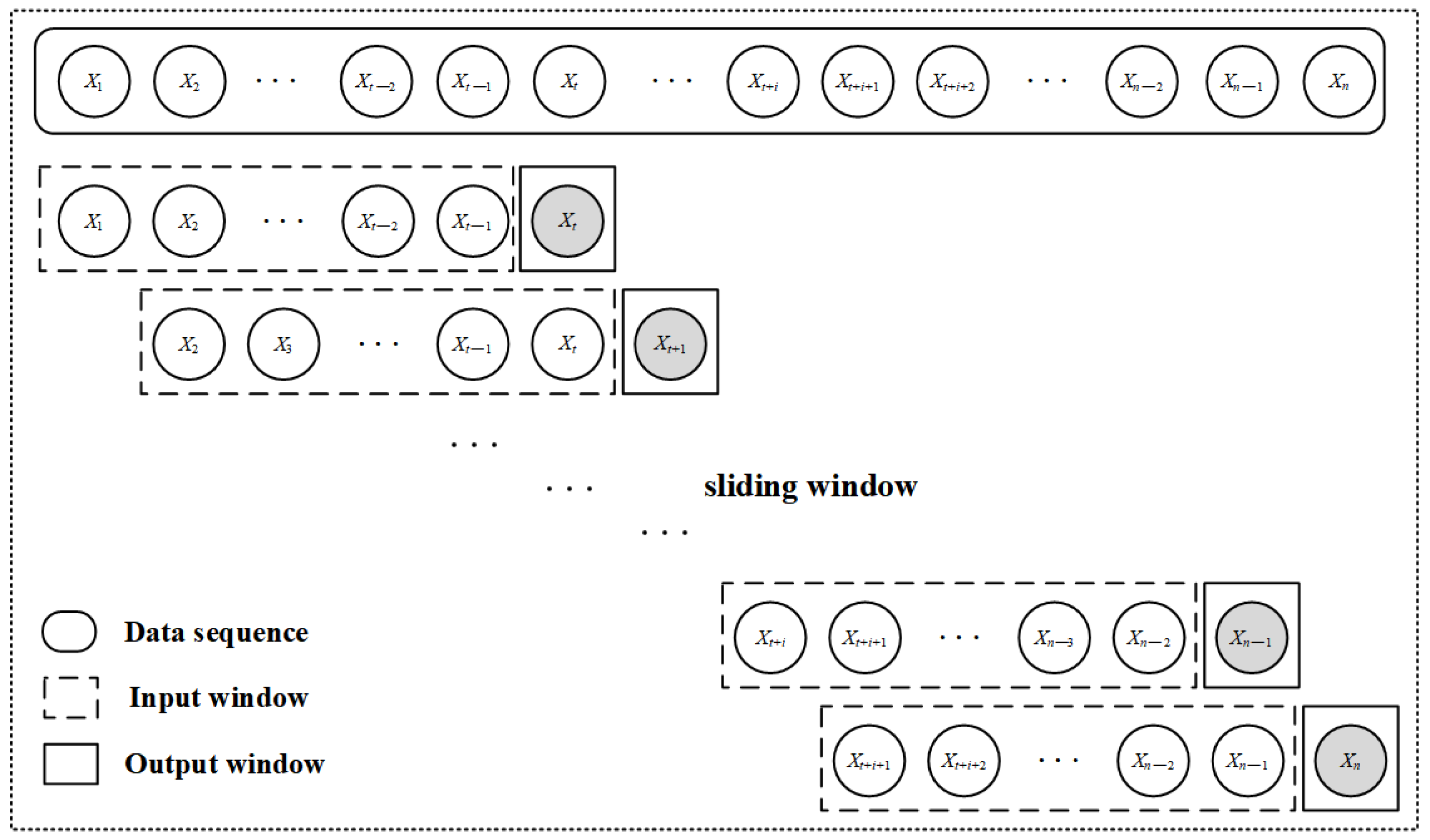
2.2. Feature Extraction and Sample Processing

Given the pivotal role of input feature preparation in establishing a dependable water demand forecasting model, the selection of the feature matrix must be carried out with precision. For short-term water demand predictions, often involving intervals as frequent as hours or minutes, input selection typically encompasses previous water demand data and climatic conditions [30]. The multitude of factors influencing water demand complicate the forecasting task. However, practical constraints often limit water utilities from consistently recording variables beyond water consumption data, such as temperature and humidity, thus posing challenges to multi-variable approaches. In this scenario, historical water demand data emerge as the most readily available and reliable variables that water distribution entities can gather. The majority of research demonstrates that a dependable prediction model can be developed solely employing historical water demand data from prior days [21]. Accordingly, in this study, historical water demand data take precedence as the primary feature, exclusively serving as the model’s inputs. Moreover, the correlation between different historical water demand sequences and the current demand requires analysis through the MIC method, as elucidated in Section 2.1, to select highly correlated sequences as inputs.

Within the collected dataset, the presence of missing values and outliers may be attributed to external factors such as sensor obstructions and pipe bursts. Extreme data can adversely impact the model’s predictive accuracy. To address this, box-and-whisker plots were employed to identify anomalous data, and vacant values as well as anomalies were substituted with the preceding average water demand at the same instance.

Additionally, direct application of historical water demand sequence data as inputs in a deep learning model is infeasible. It necessitates the reconstruction of the input–output relationship, an essential step for deep learning model training. The sliding window approach, as depicted in Figure 2, emerges as an effective strategy. This approach transforms univariate data into a supervised learning format. Notably, the deep learning model promptly generates an output window aligned with the input time steps upon receiving a corresponding input window [31]. Subsequently, in consecutive time steps, the model assimilates inputs of the same size as the preceding time step and advances by one step [22].

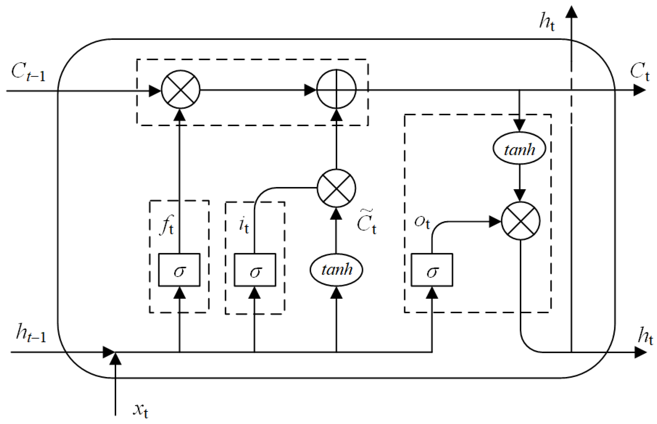
2.3. Bi-Directional Long Short Memory Network

LSTM, a specific type of RNN, effectively addresses the long-term dependency challenge and has achieved significant advancement in mitigating the vanishing or exploding gradients predicament [32]. Its fundamental unit consists of three essential logic gates: the forgetting gate, input gate, and output gate, as illustrated in Figure 3. The forgetting gate selectively discards historical information, the input gate manages the retention of present information while amalgamating it with the historical data, and the output gate determines the impact of the current state on the hidden layer. The dynamic propagation process of an LSTM cell is mathematically expressed through Equation (5) to Equation (10) [33].

$${\mathit{f}}_t=\sigma \left({\mathit{W}}_f\left[{\mathit{h}}_{t-1},{\mathit{x}}_t\right]+{\mathit{b}}_f\right)$$

(5)

$${\mathit{i}}_t=\sigma \left({\mathit{W}}_i\left[{\mathit{h}}_{t-1},{\mathit{x}}_t\right]+{\mathit{b}}_i\right)$$

(6)

$${\tilde{\mathit{C}}}_t=tanh\left({\mathit{W}}_C\left[{\mathit{h}}_{t-1},{\mathit{x}}_t\right]+{\mathit{b}}_C\right)$$

(7)

$${\mathit{C}}_t={\mathit{f}}_t{\mathit{C}}_{t-1}+{\mathit{i}}_t{\tilde{\mathit{C}}}_t$$

(8)

$${\mathit{o}}_t=\sigma \left({\mathit{W}}_o\left[{\mathit{h}}_{t-1},{\mathit{x}}_t\right]+{\mathit{b}}_o\right)$$

(9)

$${\mathit{h}}_t={\mathit{o}}_{t}tanh\left({\mathit{C}}_t\right)$$

(10)

$$X_{norm}=\frac{X_i-X_{min}}{X_{max}-X_{min}}$$

(11)

Here, ${\mathit{f}}_t,{\mathit{i}}_t,{\tilde{\mathit{C}}}_t,{\mathit{C}}_t,{\mathit{o}}_t$ represent the forget gate state, input gate state, candidate value, current cell state, and output gate state, respectively. ${\mathit{h}}_t$ is hidden layer state; ${\mathit{x}}_t$ is the input of the time; $\mathit{W},\mathit{b}$ are the corresponding weight coefficient matrix and bias vector, respectively; $\sigma ,tanh$ are the sigmod and hyperbolic tangent activation functions, respectively.

Influenced by residential water consumption patterns, water demand series typically exhibit distinct regularities, resulting in recurring or repeated patterns of demand on a daily or weekly basis. The water demand at a specific time not only relies on its immediate past demand but also reciprocally influences the water demand for its subsequent time periods. In this regard, we employ a BiLSTM network architecture to extract periodic features and capture such temporal dependencies from the historical water demand data. The structure of the BiLSTM network consists of two individual LSTM layers, one stacked on top of the other, where one processes the input data in a forward pass and the other in a backward pass [24]. This configuration allows for the learning of both forward and backward data information. Figure 4 provides an overview of the BiLSTM network’s structure employed in our model.

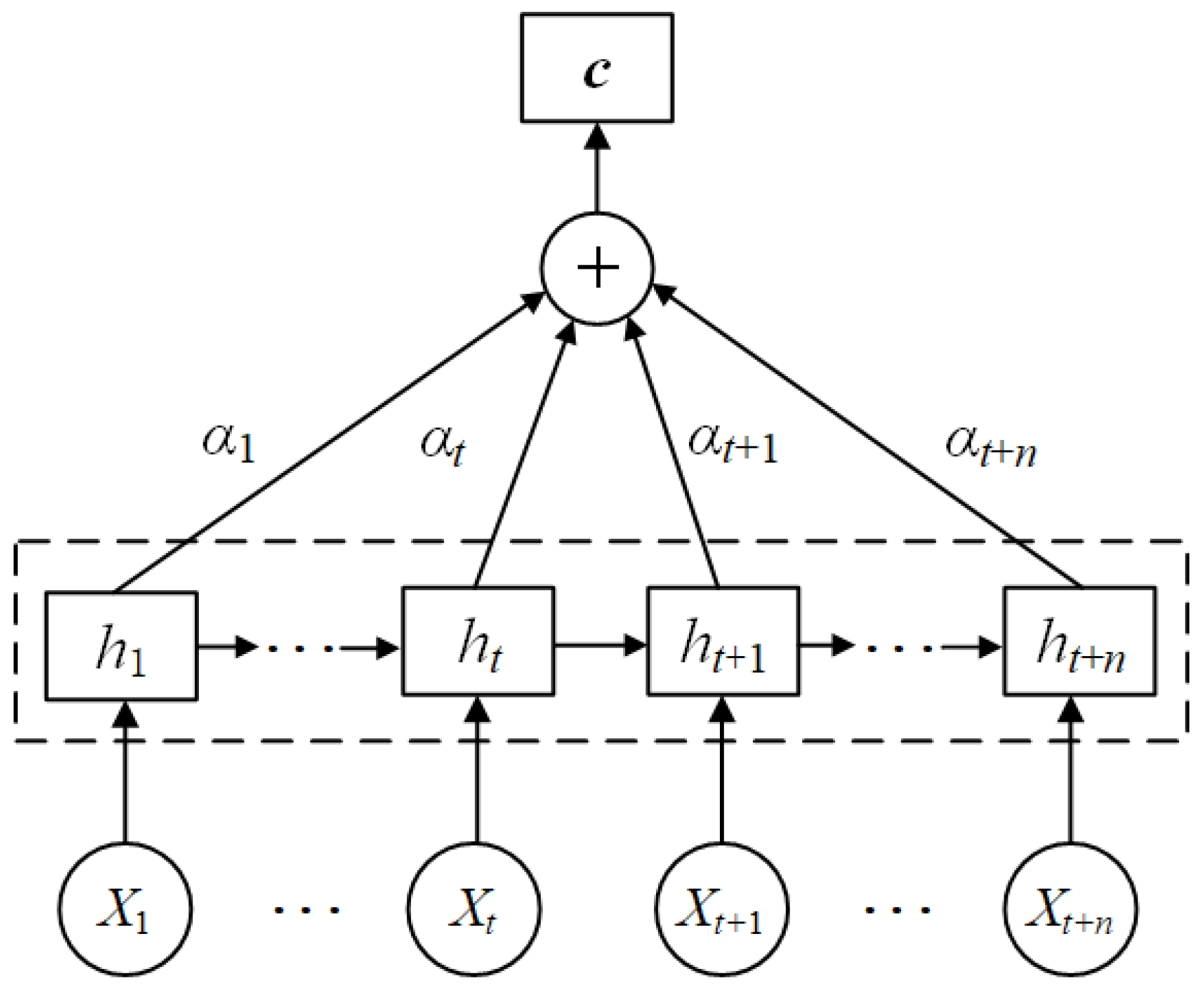
2.4. Attention Mechanism

The attention mechanism can be conceptualized as a probability distribution mechanism, assigning higher weights to features that carry more informative content [34]. This mechanism operates effectively to concentrate on crucial time steps, making the most of the information contained in each point. Its purpose is to emphasize the impact of significant factors on the present water demand. The output of the attention layer at time t can be computed using the following equation.

$${\mathit{C}}_t=\sum _{i=1}^n{\mathit{\alpha }}_i{\mathit{h}}_i$$

(12)

$${\mathit{\alpha }}_t=\frac{exp\left({\mathit{s}}_i\right)}{{\sum }_{i=1}^{n}exp\left({\mathit{s}}_i\right)}$$

(13)

$${\mathit{s}}_i=\mathit{V}tanh\left(\mathit{W}{\mathit{h}}_i+\mathit{b}\right)$$

(14)

where ${\mathit{C}}_t$ represents the output of the attention layer at time t; ${\mathit{\alpha }}_t,{\mathit{s}}_i$ are the attention weight and relevance scores, respectively; $\mathit{V},\mathit{W},\mathit{b}$ are the learnable parameters. The attention mechanism adaptively calculates and adjusts the state value of the hidden layer corresponding to the original input features to highlight important features and weaken minor features. The structure of the attention mechanism is shown in Figure 5.

2.5. XGBoost Algorithm

The fundamental concept behind the gradient boosting decision tree (GBDT) algorithm, introduced by Friedman in 2001 [35], is to employ gradient descent to generate new trees by building upon all previous trees, with the aim of minimizing the objective function. Building upon this concept, Chen et al. [36] formulated the extreme gradient boosting decision tree, known as the XGBoost algorithm. This tree ensemble model is capable of addressing classification and regression challenges. When applied to regression tasks, XGBoost generates new trees sequentially and fits the residuals of the previous model using the newly generated CART tree [37]. Distinguishing itself from GBDT, XGBoost enables parallel execution based on boosted trees and efficiently handles complex data. In this study, the XGBoost algorithm is employed for the purpose of correcting residual predictions, thereby further enhancing prediction accuracy. The objective function of XGBoost generally comprises a loss function and a regularization term, as illustrated below.

$$Obj\left(\theta \right)=\sum _{i=1}^{k}L\left({\widehat{y}}_i,y_i\right)+\sum _{i=1}^k\Omega \left(f_k\right)$$

(15)

where $L\left({\widehat{y}}_i,y_i\right)$ represents the training loss function; $\Omega \left(f_k\right)$ is the regularization term; ${\widehat{y}}_i,y_i$ are predicted and actual values, respectively; k is the number of trees, $f_k$ is the k th tree, the sum of results corresponding to each tree is used as the predicted results [38].

The regularization term is used to control the complexity of the model and can be illustrated using the following expression:

$$\Omega \left(f\right)=\gamma T+\frac{1}{2}\lambda {∥w∥}^2$$

(16)

where T represents the number of leaves; $\gamma$ and $\lambda$ are penalty coefficients; w is the vector of scores on leaves.

The objective function of XGBoost undergoes a quadratic Taylor expansion and omits higher-order infinitesimal quantities. It is further simplified and defined as:

$$Obj\left(\theta \right)=\sum _{i=1}^T\left[G_j{w}_j+\frac{1}{2}(H_j+\lambda w_j^2)\right]+\gamma T$$

(17)

where $G_j={\sum }_{iϵIj}^{}{g}_j,H_j={\sum }_{iϵIj}^{}{h}_j$, and $g_j=\partial {\widehat{y}}^{(t-1)}L(y_i,{\widehat{y}}_i^{(t-1)}),h_j={\partial }^2{\widehat{y}}^{(t-1)}L(y_i,{\widehat{y}}_i^{(t-1)})$. $w_j$ are independent from each other. Then, rewriting Equation (16) to the quadratic function of one variable related to $w_j$, we obtain the optimal solution of $w_j$ that is equal to $-\frac{G_j}{H_j+\lambda }$. Substituting this into Equation (16), the objective function is finally as follows:

$$Obj\left(\theta \right)=-\sum _{i=1}^T\frac{G_j^2}{H_j+\lambda }+\lambda T$$

(18)

2.6. Performance Metrics of Forecast Models

Statistical standard parameters provide an alternative to evaluate the prediction accuracy of the model. An effective model does not only require good forecasting ability but also possesses stability. That is to say, it is necessary to utilize multi-evaluation metrics for observing the quality of the model. Thus, the performances of various models are analyzed in this study with four criteria that are commonly used in water demand forecasting: mean absolute error (MAE), root mean square error (RMSE), mean absolute percentage error (MAPE), and Nash–Sutcliffe Model Efficiency (NSE), which are calculated according to Equations (19)–(22), respectively [7].

$$MAE=\frac{1}{N}\sum _{i=1}^N|Y_i-{\widehat{Y}}_i|$$

(19)

$$MAPE=\frac{100}{N}\sum _{i=1}^N|\frac{Y_i-{\hat{Y}}_i}{Y_i}|$$

(20)

$$\mathrm{RMSE}=\sqrt{\frac{1}{N}\sum _{i=1}^N{\left(Y_i-{\hat{Y}}_i\right)}^2}$$

(21)

$$\mathrm{NSE}=1-\frac{{\sum }_{i=1}^N{\left(Y_i-{\widehat{Y}}_i\right)}^2}{{\sum }_{i=1}^N{\left(Y_i-{\stackrel{\_}{Y}}_i\right)}^2}$$

(22)

where $Y_i$ is the observed value; ${\widehat{Y}}_i$ is the forecasted value; $Y_i$ is the mean of the observed value. According to the evaluation metrics, lower values of MAE, MAPE, and RMSE refer to a better model performance, whereas higher NSE values reveal better models. In particular, MAPE is the relative value without unit, and its value range is $[0,+\infty ]$. The closer the value is to 0, the more perfect the model is. NSE can generally explain the stability and fitting effect of the model; the closer the value is to 1, the more stable the model is.

3. Case Study

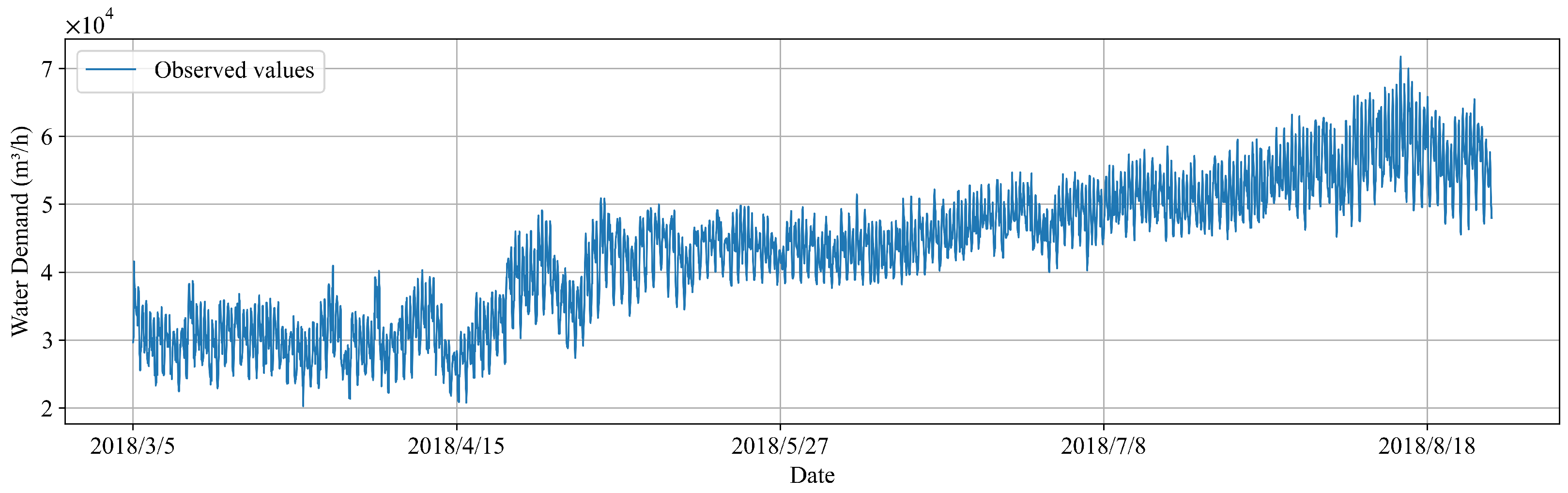
3.1. Dataset Description

The water demand data were gathered from a municipal water distribution system in a southern Chinese city spanning from5 March 2018 to 26 August 2018 with a 1 h interval. The water distribution dataset after undergoing data cleaning is depicted in Figure 6. This dataset encapsulates the diverse water consumption of various users within the region. The objective of this study is to apply the proposed method to predict water demand 1 h ahead, effectively constituting a one-step prediction. Prior to assessing the efficacy of the proposed approach, preprocessing of data and extraction of features were conducted.

Guided by the MIC method, historical sequences that significantly impact current water demands were identified. Representatively, $P(w,d,h)$ signifies water demand at a specific hour of a given week’s day. Consequently, $P(w,d,h-1)$ denotes water demand for the preceding hour of the same day and week; $P(w,d-1,h)$ denotes water demand for the same hour on a prior day of the week; $P(w-1,d,h)$ signifies water demand for the same hour of the day in the preceding week. Other parameters follow analogous patterns. Acknowledging the daily and weekly periodicities in water demand, the MIC values of seven correlated features were computed (

Table 1. Correlation between historical water demand and current water demand.

Label	Sequences	MIC
P1	$P(w,d,h-1)$	0.863
P2	$P(w,d,h-2)$	0.755
P3	$P(w,d,h-3)$	0.704
P4	$P(w,d-1,h)$	0.792
P5	$P(w,d-1,h-1)$	0.766
P6	$P(w-1,d,h)$	0.783
P7	$P(w-1,d,h-1)$	0.708

). These inputs were amalgamated to enhance the efficacy of model training. Notably, all MIC values exceed 0.7, signifying a robust temporal dependence between the chosen historical series and current water demand. Consequently, these features were aptly selected as model inputs. Of note, with the closest temporal relationship, the sequence $P(w,d,h-1)$ bears the highest relevance to the sequence $P(w,d,h)$. For the sake of subsequent reference, we will denote these sequences as P1 to P7.

Subsequently, the sliding window strategy was employed to reconfigure the data into a supervised learning pattern. Simultaneously, the complete dataset was partitioned into training, validation, and test subsets. To expedite model convergence while retaining data’s statistical characteristics, values were independently normalized in the divided datasets using Equation (11). In this regard, the training phase encompassed data from the previous 105 days (equivalent to 15 weeks), the validation phase encompassed data from 35 days (equivalent to 5 weeks), and the remaining data (5 weeks) were allocated to the test phase. This approach effectively prevents data information leakage and facilitates the networks’ generalization ability assessment on the test dataset. Furthermore, data shuffling was executed before each training epoch to prevent bias in data manipulation.

3.2. Model Parameter Configuration

A robust prediction model hinges not only on its architectural design but also on astute hyper-parameter configurations. Aptly chosen hyper-parameters empower the model to aptly capture the intricacies of the data, thus yielding effective results while mitigating computational burden.

Concerning the BiLSTM model, several hyper-parameters warrant careful configuration: (1) the number of BiLSTM layers; (2) the quantity of neurons in each layer; (3) the learning rate; (4) the activation function; (5) the inclusion of the dropout layer. Employing excessive layers and neurons risks creating a model too intricate for efficient training and computational feasibility. Conversely, overly simplistic settings could yield unexpected predictions [21]. Furthermore, selecting the optimal number of training epochs for the model is crucial. In this study, an early stopping training strategy was employed to optimize computational time by evaluating the convergence and stability of training and validation losses.

Hyper-parameters for the BiLSTM model were determined through random search using Keras Tuner. Keras Tuner, a scalable hyper-parameter optimization framework, addresses the challenges of hyper-parameter search by integrating built-in Bayesian optimization, hyperband, and random search algorithms [39]. Random search, compared to conventional grid search and manual search, constitutes a more efficient hyper-parameter optimization method [40]. We employed the mean square error (MSE) as the evaluation metric, configuring parameters within the search range to minimize the MSE. Through three experimental trials conducted using Keras Tuner, we obtained the optimal parameter configuration results, as presented in

Table 2. The hyper-parameter search range and optimal configuration of the BiLSTM model.

Hyper-Parameter	Search Range	BiLSTM
Number of layers	[1, 2, 3]	2
Number of neurons	from 32 to 128 with an increase 16	64
Learning rate	ranging from 0.0001 to 0.01 with an increase of 0.0001	0.0043
Activation	tanh, ReLU	ReLU
Dropout	True or False	False

.

In terms of the XGBoost model, there are three categories of parameters requiring configuration. These encompass general parameters, booster parameters, and task parameters. General parameters pertain to the choice of booster utilized for boosting, typically involving a tree or linear model. Booster parameters vary based on the specific booster selected, while learning task parameters determine the learning scenario and task at hand [41].

Our primary focus centers on the booster parameters, as these parameters, among the three types mentioned, exert the most influential impact on fitting performance. In this context, random search is also employed to identify optimal parameters, including: (1) n_estimators; (2) max_depth; (3) gamma; (4) eta, alias learning rate; (5) subsample; (6) colsample_bytree. The search range for these six parameters, along with the optimal configuration of the XGBoost model, is detailed in

Table 3. The hyper-parameter search range and optimal configuration of the XGBoost model.

Hyper-Parameter	Search Range	XGBoost
n_estimators	ranging from 100 to 150	100
max_depth	[2, 3, 4, 5, 6]	6
eta	ranging from 0.01 to 0.3 with an increase of 0.01	0.3
gamma	[0, 1, 2, 3]	0
subsample	ranging from 0.5 to 1 with an increase of 0.1	0.8
colsample_bytree	ranging from 0.5 to 1 with an increase of 0.1	1

. Other parameters within this model, not elaborated upon here, adopt default values.

3.3. Results and Discussion

As part of the objectives of this study, the utilization of the BiLSTM model was pivotal in capturing bidirectional information inherent in water demand series. Therefore, in this context, the LSTM model was also employed for forecasting purposes. The intention was to gauge the performance enhancement offered by the BiLSTM model. The parameter configurations for the LSTM model mirrored those of the BiLSTM model. Furthermore, the incorporation of an attention mechanism into the BiLSTM network architecture aimed to accentuate the critical information pertinent to the current water demand. This led to the creation of the Attention-BiLSTM model, dedicated to water demand forecasting. To amplify the prediction accuracy of the model, we calculated the discrepancy between the observed and predicted values of the Attention-BiLSTM model on the training dataset. These discrepancies were considered as the output of the XGBoost model. Subsequently, this error, simulated by the XGBoost model, was employed to refine the fitting outcomes of the Attention-BiLSTM model, yielding the ultimate forecasted values. All model developments were conducted within the Python environment.

3.3.1. Analysis of Attention Mechanism

To investigate the impact of the attention mechanism on predictive models, the 6 weeks water demand dataset was selected, and the attention weights assigned to different input features are illustrated in Figure 7.

As observed from Figure 7, the attention mechanism establishes connections between different input feature sequences and their impact on the predictive outcomes. Among these, the model assigns the highest attention weight to the previous moment’s load sequence, $P(w,d,h-1)$, indicating its significant influence on the current load prediction. Conversely, the weight coefficient for $P(w,d,h-3)$ is the smallest, signifying its minimal impact on the prediction outcomes. In Figure 8, as the time span of the selected dataset increases from 7 days to 77 days, changes in the attention weights corresponding to each input sequence are depicted. The graph reveals that the attention weights for each input sequence dynamically fluctuate and gradually stabilize as the time span expands. The attention mechanism does not merely average the contribution rates of various influencing factors; rather, it autonomously explores the degree of influence of different input features on the prediction results at each moment. This enhances the model’s capability to extract key feature information.

3.3.2. Comparison of Predictive Performance among Various Models

Performance metrics derived from the test dataset for the proposed method have been consolidated in

Table 4. Performance metrics of forecast models on test dataset.

Model	MAE (m3/h)	RMSE (m3/h)	MAPE (%)	NSE
Proposed method	544	915	1.00	0.99
Attention-BiLSTM	1128	1405	1.95	0.92
BiLSTM	1145	1475	2.00	0.88
LSTM	1235	1576	2.14	0.85

. A comprehensive review of the table underscores the noteworthy efficacy of the Attention-BiLSTM networks combined with the XGBoost model across all assessment criteria. This affirms that the suggested forecasting approach not only exhibits superior predictive prowess but also showcases commendable robustness when compared to the spectrum of benchmark models.

Delving into the specifics, juxtaposing the BiLSTM model with the LSTM model reveals a 0.14% reduction in MAPE and a 6.3% augmentation in prediction accuracy. Moreover, the stability of the prediction, as indicated by NSE, escalates from 0.85 to 0.88. This suite of metrics collectively substantiates the superior performance of the BiLSTM model in deciphering bidirectional data dynamics within water demand series, consequently leading to enhanced predictive precision.

Building on this foundation, the augmentation of the BiLSTM model through the incorporation of an attention mechanism further refines prediction accuracy and stability. The MAPE of the Attention-BiLSTM model registers a 0.05% decrease compared to its BiLSTM counterpart, while attaining an NSE of 0.92. It is pertinent to note that while the performance enhancement may seem marginal, it can be reasonably attributed to the selective feature extraction achieved by the MIC method, combined with the comprehensive data insight harnessed by the BiLSTM model. This confluence leaves limited room for improvement through the attention layer. Nevertheless, this marginal boost conclusively underscores the role of the attention mechanism in accentuating pivotal information within historical sequences, thereby fortifying the predictive efficacy of the networks, particularly when the input features and underlying data dynamics are adeptly captured.

Moreover, the proposed method, which incorporates a residual correction module, consistently demonstrates remarkable performance in terms of both forecast accuracy and model stability. The substantial leap in performance is evident from the evaluation criteria, where the proposed method achieves an impressive MAPE of 1.0%. This improvement is remarkable, surpassing 48.7%, 50.0%, and 53.3% in comparison to the Attention-BiLSTM model and two other deep learning models, respectively. Additionally, the RMSE metrics exhibit substantial reductions of 41.9%, 37.9%, and 34.8% when compared to the LSTM, the BiLSTM, and the Attention-BiLSTM models, respectively. The NSE improvement is equally notable, nearly reaching a perfect score of 0.99.

These metric values unequivocally highlight the substantial contribution of the residual correction module to the enhanced forecast accuracy. Essentially, the utilization of the XGBoost algorithm to simulate errors greatly aids in rectifying final forecasted results. Particularly, the module addresses data fluctuations that are inherently challenging for deep learning models to capture.

An illustration depicting the forecasted water demand curves of the proposed method and other benchmark models is presented in Figure 9. The architecture of deep learning models demonstrates a clear advantage in processing nonlinear data, closely mirroring the trend of the water demand series. Notably, the proposed method excels in predicting points of significant demand fluctuations, especially during peak hours, which holds pivotal importance for water distribution scheduling. Moreover, the forecast curve of the proposed method closely aligns with the actual water demand curve due to the influence of the residual simulations facilitated by the Attention-BiLSTM networks.

3.3.3. Contrast with Previous Studies

In this study, the coupling of the attention mechanism with the BiLSTM model was attempted, introducing it into the field of short-term water demand forecasting. By employing the XGBoost algorithm to simulate the dataset’s errors, the aim was to enhance the predictive accuracy of the model. This novel approach presents a new framework for short-term water demand prediction. Contrasted with prior research, this represents a fresh hybrid model that encompasses the entire process chain of short-term water demand forecasting. It avoids the previous challenges of intuitively selecting input features and manually enumerating model parameters for comparison. The approach significantly addresses model error issues that deep learning models often overlook, resulting in a noteworthy improvement in performance—an aspect largely unexplored in many previous studies [2,4,7,22].

Simultaneously, when the input features of the model are effectively chosen, the impact of using the attention mechanism may diminish. In other words, the potential for performance enhancement through the application of the attention mechanism becomes limited. To elaborate, the application of the attention mechanism was followed by a preliminary screening of model input features using the MIC method. This selection of crucial features, combined with the subsequent integration of the attention mechanism, effectively presents a two-tier filtering process for these features. This phenomenon is reflected in the performance metrics seen in Table 4. Notably, the model’s performance is enhanced on this foundation, albeit with marginal improvement potential.

This outcome offers a potential avenue for future research, especially regarding the influence of feature selection on model performance. Within the current context of utilizing the attention mechanism for predicting traffic and electricity demands, this aspect seems to have been largely overlooked [24,25].

4. Conclusions

In order to address the instability associated with short-term water demand forecasting, particularly with a time resolution of 1 h, we have introduced a novel machine learning-based model framework. Our intention is to provide a novel perspective and reference for short-term water demand prediction within the scope of smart water management systems, ultimately aiming to serve short-term water resource scheduling needs.

Initially, we explored the application of the MIC method for feature extraction, aiming to select high-quality inputs for our model. Additionally, we transformed univariate data into a supervised learning pattern using a sliding window scheme, which is suitable for the architecture. Subsequently, we synergistically harnessed the advantages of BiLSTM, the attention mechanism, and the XGBoost algorithm to create an innovative forecasting approach. This proposed hybrid model was evaluated using an hourly water demand dataset collected from the water supply system in a city in South China. We employed the random parameter search algorithm of Keras Tuner for optimizing hyper-parameters in the deep learning models, and the same approach was used to determine the hyper-parameter configuration for the XGBoost model. To demonstrate the superiority of our approach, we compared it with the LSTM, BiLSTM, and Attention-BiLSTM models to gauge the degree of improvement achieved.The conclusions drawn from this studyare as follows:

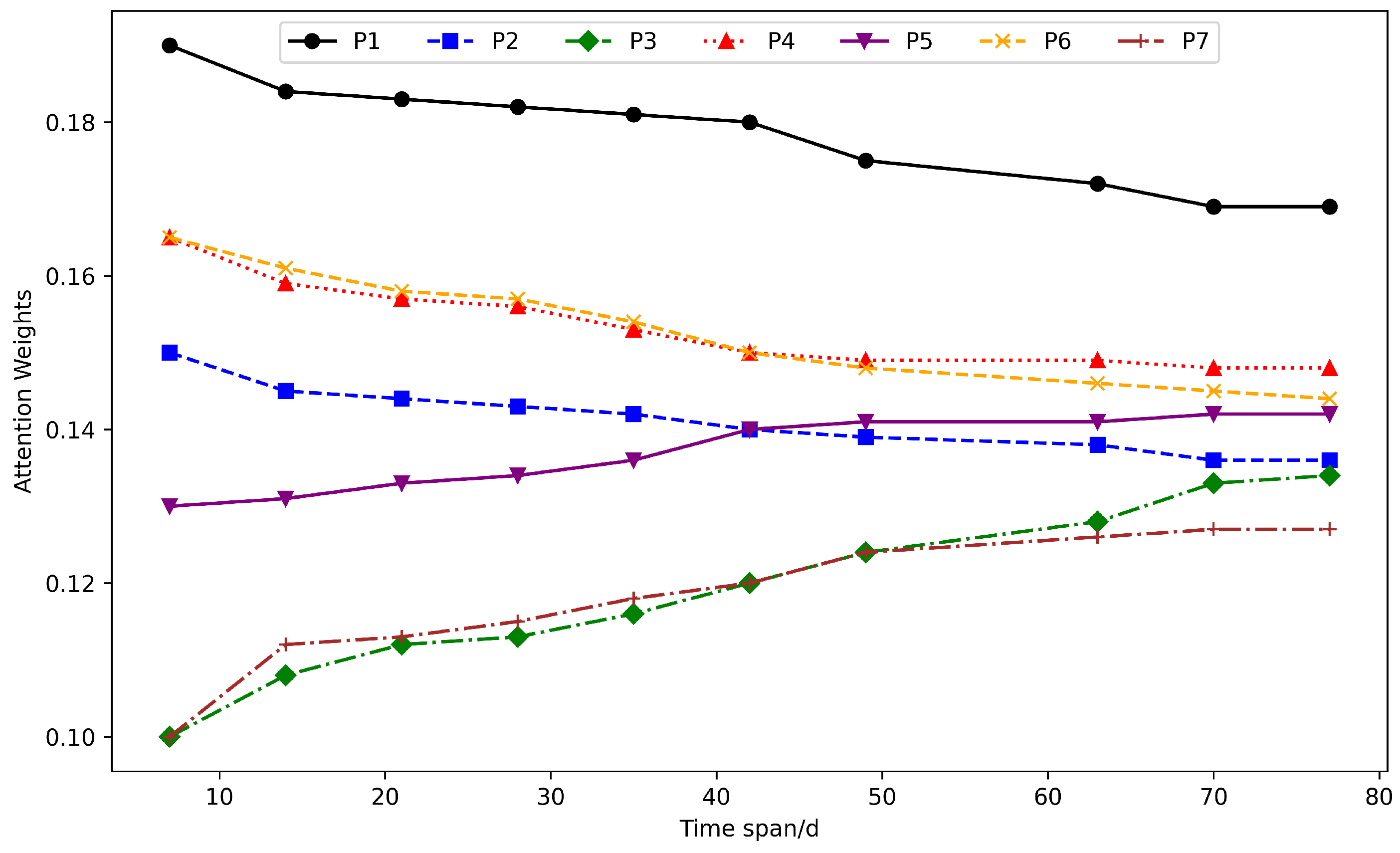
(1)

The attention mechanism exerts a significant influence on linking various input feature sequences to their impact on predictive outcomes. It assigns varying weights to different sequences, with those containing more vital information receiving higher weights. Furthermore, as the temporal span of the dataset extends, the attention weights for each input sequence gradually stabilize amidst dynamic fluctuations. Importantly, the attention mechanism surpasses mere averaging of contribution rates across factors; rather, it autonomously explores the effect of distinct input features on predictive outcomes at each instance. This inherent mechanism notably strengthens the model’s capacity to extract pivotal feature information, thereby facilitating superior predictions.

(2)

In terms of the MAE, MAPE, RMSE, and NSE evaluation indicators, the results clearly demonstrate that the proposed method achieves state-of-the-art predictions and exhibits the highest level of robustness across all model tests. The proposed method excels in performance on the test dataset, with MAE, RMSE, MAPE, and NSE values of 544 m³/h, 915 m³/h, 1.00%, and 0.99, respectively, outperforming other benchmark models significantly. Therefore, it can be concluded that our approach is both valid and superior, showcasing satisfactory generalization ability, which could be instrumental in the development of a smart water demand consumption forecasting system.

(3)

In this dataset, when the model’s input features are effectively selected, the impact of the attention mechanism might be attenuated. This means that the potential for improvement in model predictive performance could be relatively reduced. In essence, by applying the MIC method to filter the model’s input features, the critical features that are selected undergo a secondary refinement upon integration with the attention mechanism. Consequently, while the model’s performance is indeed enhanced on this foundation, the scope for further enhancement is limited.

It is important to note, however, that this research specifically focuses on one-hour ahead water demand forecasting and does not delve into multi-step predictions. However, it is worth acknowledging that multi-step forecasting is essentially an extension of the one-step forecast. As part of future work, it is imperative to explore the effectiveness of the proposed architecture in this study for multi-step forecasting of water demand. In addition, constrained by data availability, the relatively short time span of the dataset may impose limitations on the model’s performance and generalization across various seasons and years. In the future, it is advisable to expand and validate the model with additional training datasets in practical applications.

References

- Wu, Y.; Zhang, W.; Shen, J.; Mo, Z.; Yi, P. Smart city with Chinese characteristics against the background of big data: Idea, action and risk. J. Clean. Prod. 2017, 173, 60–66. [Google Scholar] [CrossRef]
- Huang, H.; Zhang, Z.; Song, F. An Ensemble-Learning-Based Method for Short-Term Water Demand Forecasting. Water Resour. Manag. 2021, 35, 1757–1773. [Google Scholar] [CrossRef]
- Herrera, M.; Torgo, L.; Izquierdo, J.; Pérez-García, R. Predictive models for forecasting hourly urban water demand. J. Hydrol. 2010, 387, 141–150. [Google Scholar] [CrossRef]
- Sebri, M. Forecasting urban water demand: A meta-regression analysis. J. Environ. Manag. 2016, 183, 777–785. [Google Scholar] [CrossRef]
- Donkor, E.A.; Mazzuchi, T.A.; Soyer, R.; Roberson, J.A. Urban Water Demand Forecasting: Review of Methods and Models. J. Water Resour. Plan. Manag. 2014, 140, 146–159. [Google Scholar] [CrossRef]
- Tiwari, M.K.; Adamowski, J. Urban water demand forecasting and uncertainty assessment using ensemble wavelet-bootstrap-neural network models. Water Resour. Res. 2013, 49, 6486–6507. [Google Scholar] [CrossRef]
- Guo, G.; Liu, S.; Wu, Y.; Li, J.; Zhou, R.; Zhu, X. Short-Term Water Demand Forecast Based on Deep Learning Method. J. Water Resour. Plan. Manag. 2018, 144, 04018076. [Google Scholar] [CrossRef]
- Rak, J.R.; Tchórzewska-Cieślak, B.; Pietrucha-Urbanik, K. A hazard assessment method for waterworks systems operating in self-government units. Int. J. Environ. Res. Public Health 2019, 16, 767. [Google Scholar] [CrossRef]
- Liu, X.; Sang, X.; Chang, J.; Zheng, Y. Multi-model coupling water demand prediction optimization method for megacities based on time series decomposition. Water Resour. Manag. 2021, 35, 4021–4041. [Google Scholar] [CrossRef]
- Braun, M.; Bernard, T.; Piller, O.; Sedehizade, F. 24-Hours Demand Forecasting Based on SARIMA and Support Vector Machines. Procedia Eng. 2014, 89, 926–933. [Google Scholar] [CrossRef]
- Kofinas, D.; Mellios, N.; Papageorgiou, E.; Laspidou, C. Urban Water Demand Forecasting for the Island of Skiathos. Procedia Eng. 2014, 89, 1023–1030. [Google Scholar] [CrossRef]
- Oliveira, P.J.; Steffen, J.L.; Cheung, P. Parameter Estimation of Seasonal Arima Models for Water Demand Forecasting Using the Harmony Search Algorithm. Procedia Eng. 2017, 186, 177–185. [Google Scholar] [CrossRef]
- Ma, X.; Jin, Y.; Dong, Q. A generalized dynamic fuzzy neural network based on singular spectrum analysis optimized by brain storm optimization for short-term wind speed forecasting. Appl. Soft Comput. 2017, 54, 296–312. [Google Scholar] [CrossRef]
- Wong, J.S.; Zhang, Q.; Chen, Y.D. Statistical modeling of daily urban water consumption in Hong Kong: Trend, changing patterns, and forecast. Water Resour. Res. 2010, 46, 3. [Google Scholar] [CrossRef]
- Niknam, A.; Zare, H.K.; Hosseininasab, H.; Mostafaeipour, A.; Herrera, M. A Critical Review of Short-Term Water Demand Forecasting Tools—What Method Should I Use? Sustainability 2022, 14, 5412. [Google Scholar] [CrossRef]
- Xenochristou, M.; Hutton, C.; Hofman, J.; Kapelan, Z. Water Demand Forecasting Accuracy and Influencing Factors at Different Spatial Scales Using a Gradient Boosting Machine. Water Resour. Res. 2020, 56, e2019WR026304. [Google Scholar] [CrossRef]
- Salloom, T.; Yu, X.; He, W.; Kaynak, O. Adaptive Neural Network Control of Underwater Robotic Manipulators Tuned by a Genetic Algorithm. J. Intell. Robot. Syst. 2019, 97, 657–672. [Google Scholar] [CrossRef]
- Ding, C.; Tao, D. Robust Face Recognition via Multimodal Deep Face Representation. IEEE Trans. Multimed. 2015, 17, 2049–2058. [Google Scholar] [CrossRef]
- Minaee, S.; Kalchbrenner, N.; Cambria, E.; Nikzad, N.; Chenaghlu, M.; Gao, J. Deep Learning—Based Text Classification: A Comprehensive Review. ACM Comput. Surv. 2021, 54, 3. [Google Scholar] [CrossRef]
- Zhao, Z.Q.; Zheng, P.; Xu, S.T.; Wu, X. Object Detection With Deep Learning: A Review. IEEE Trans. Neural Networks Learn. Syst. 2019, 30, 3212–3232. [Google Scholar] [CrossRef]
- Zanfei, A.; Menapace, A.; Granata, F.; Gargano, R.; Frisinghelli, M.; Righetti, M. An Ensemble Neural Network Model to Forecast Drinking Water Consumption. J. Water Resour. Plan. Manag. 2022, 148, 04022014. [Google Scholar] [CrossRef]
- Chen, L.; Yan, H.; Yan, J.; Wang, J.; Tao, T.; Xin, K.; Li, S.; Pu, Z.; Qiu, J. Short-term water demand forecast based on automatic feature extraction by one-dimensional convolution. J. Hydrol. 2022, 606, 127440. [Google Scholar] [CrossRef]
- Bahdanau, D.; Cho, K.; Bengio, Y. Neural Machine Translation by Jointly Learning to Align and Translate. arXiv 2014, arXiv:1409.0473. [Google Scholar] [CrossRef]
- Zheng, H.; Lin, F.; Feng, X.; Chen, Y. A Hybrid Deep Learning Model With Attention-Based Conv-LSTM Networks for Short-Term Traffic Flow Prediction. IEEE Trans. Intell. Transp. Syst. 2020, 22, 6910–6920. [Google Scholar] [CrossRef]
- Wang, J.; Du, C. Short-term load prediction model based on Attention-BiLSTM neural network and meteorological data correction. Electr. Power Autom. Equip. 2022, 42, 7. [Google Scholar] [CrossRef]
- Du, B.; Huang, S.; Guo, J.; Tang, H.; Wang, L.; Zhou, S. Interval forecasting for urban water demand using PSO optimized KDE distribution and LSTM neural networks. Appl. Soft Comput. 2022, 122, 108875. [Google Scholar] [CrossRef]
- Guo, J.; Sun, H.; Du, B. Multivariable time series forecasting for urban water demand based on temporal convolutional network combining random forest feature selection and discrete wavelet transform. Water Resour. Manag. 2022, 36, 3385–3400. [Google Scholar] [CrossRef]
- Duerr, I.; Merrill, H.R.; Wang, C.; Bai, R.; Boyer, M.; Dukes, M.D.; Bliznyuk, N. Forecasting urban household water demand with statistical and machine learning methods using large space-time data: A Comparative study. Environ. Model. Softw. 2018, 102, 29–38. [Google Scholar] [CrossRef]
- Kinney, J.B.; Atwal, G.S. Equitability, mutual information, and the maximal information coefficient. Proc. Natl. Acad. Sci. USA 2014, 111, 3354–3359. [Google Scholar] [CrossRef]
- Nunes Carvalho, T.M.; Filho, F. Variational Mode Decomposition Hybridized With Gradient Boost Regression for Seasonal Forecast of Residential Water Demand. Water Resour. Manag. 2021, 35, 3431–3445. [Google Scholar] [CrossRef]
- Smyl, S. Forecasting Short Time Series with LSTM Neural Networks. 2016. Available online: https://gallery.azure.ai/Tutorial/Forecasting-Short-Time-Series-with-LSTM-Neural-Networks-2 (accessed on 1 August 2023).
- Nguyen, H.P.; Liu, J.; Zio, E. A long-term prediction approach based on long short-term memory neural networks with automatic parameter optimization by Tree-structured Parzen Estimator and applied to time-series data of NPP steam generators. Appl. Soft Comput. 2020, 89, 106116. [Google Scholar] [CrossRef]
- Sherstinsky, A. Fundamentals of recurrent neural network (RNN) and long short-term memory (LSTM) network. Phys. D Nonlinear Phenom. 2020, 404, 132306. [Google Scholar] [CrossRef]
- Gao, J.; Gao, X.; Wu, N.; Yang, H. Bi-directional LSTM with multi-scale dense attention mechanism for hyperspectral image classification. Multimed. Tools Appl. 2022, 81, 24003–24020. [Google Scholar] [CrossRef]
- Friedman, J.H. Greedy Function Approximation: A Gradient Boosting Machine. Ann. Stat. 2001, 29, 1189–1232. [Google Scholar] [CrossRef]
- Chen, T.; Tong, H.; Benesty, M. Xgboost: Extreme Gradient Boosting. 2016. Available online: https://cran.ms.unimelb.edu.au/web/packages/xgboost/vignettes/xgboost.pdf (accessed on 3 August 2023).
- Pan, S.; Zheng, Z.; Guo, Z.; Luo, H. An optimized XGBoost method for predicting reservoir porosity using petrophysical logs. J. Pet. Sci. Eng. 2022, 208, 109520. [Google Scholar] [CrossRef]
- Nguyen, H.; Bui, X.N.; Bac, B.; Cuong, D. Developing an XGBoost model to predict blast-induced peak particle velocity in an open-pit mine: A case study. Acta Geophys. 2019, 67, 477–490. [Google Scholar] [CrossRef]
- Saleh, H.; Mostafa, S.; Alharbi, A.; El-Sappagh, S.; Alkhalifah, T. Heterogeneous Ensemble Deep Learning Model for Enhanced Arabic Sentiment Analysis. Sensors 2022, 22, 3707. [Google Scholar] [CrossRef]
- Bergstra, J.; Bengio, Y. Random Search for Hyper-Parameter Optimization. J. Mach. Learn. Res. 2012, 13, 281–305. [Google Scholar] [CrossRef]
- Chen, Z.; Liu, J.; Li, C.; Ji, X.; Li, D.; Huang, Y.; Di, F.; Gao, X.; Xu, L. Ultra Short-term Power Load Forecasting Based on Combined LSTM-XGBoost Model. Power Syst. Technol. 2020, 44, 614–620. [Google Scholar] [CrossRef]