A Multi-Factor Combination Model for Medium to Long-Term Runoff Prediction Based on Improved BP Neural Network

Abstract

Taking a certain coastal area of Jiangsu province as the research background, this study scientifically predicts the runoff on the medium and long-term time scale according to the changes of various climate factors such as atmospheric circulation, sea surface temperature, and solar activity in the first half of the year. A lag correlation is established between various related climate factors and the monthly runoff process in the research area for the previous 1–6 months. Selecting advantageous factors and constructing a significant factor set. Using the improved BP (Back-Propagation) artificial neural network model and combining it with the sensitivity analysis method, a specific number of 8-factor combinations are selected from the set of significant factors for medium and long-term runoff prediction. After that, the prediction results are compared with the forecasting effects of two multi-factor combination runoff simulation schemes formed by stepwise regression and Spearman rank correlation methods. The study concluded that the multi-factor combination simulation effect formed through sensitivity analysis was the best. The 20% standard forecast qualification rate of the three schemes is not significantly different. The Mean Absolute Relative Error of the multi-factor combination training and validation periods simulated through sensitivity analysis is the smallest among the three schemes, which are 36.61% and 38.01%, respectively. The Nash Efficiency Coefficient in the validation period is 0.45, which is far better than other schemes and has better generalization ability. The Standard Deviation of Relative Error in the training and validation periods is much smaller than other schemes, and the dispersion of relative errors is the smallest.

1. Introduction

Runoff volume, a significant source of water resource management, has been studied for over half a century [1]. Accurate prediction of runoff is crucial for effective water resources management, agricultural irrigation, flood warning systems, and hydropower generation. The intricate interplay between vegetation and precipitation has gained widespread recognition. Considering the limitations imposed by water availability on ecosystem functioning, precise runoff prediction can facilitate optimal ecological restoration under limited water conditions and serve as a decision-making basis for vegetation restoration in diverse regions [2,3]. During the melting process, substantial amounts of snow-melt runoff enter rivers, potentially leading to flooding. Shigemi Hatta proposed the use of weekly weather forecast data in snowmelt runoff prediction, which was calculated based on sunshine percentage at that time when solar activity was not well understood [4]. Subsequently, researchers have explored more variables such as topography, geology, air temperature, precipitation, and watershed area to improve the accuracy of flood damage avoidance predictions [5]. In recent years, with richer meteorological and surface parameter data as well as remote sensing technology available, progress has also been made in data quality control and preprocessing techniques for research purposes. H.V. Trivedi pioneered the application of grey system theory in hydrology to model runoff prediction with good practical effects using only a small set of hydrological data required for flow prediction [6].

Due to the complex characteristics of the runoff process, such as time-varying and non-stationary behavior, the selection of a leading predictor plays a crucial role in accurately predicting runoff. The prediction of runoff performance can potentially be influenced by the addition of rainfall factors and underlying surface [7,8]. Rai’s study on overland roughness found that hydrological curves with different land roughness were consistent with observed runoff hydrological curves [9]. Samantaray discovered that predicting runoff always relies on five data items, including rainfall, temperature, stage, specific humidity, and relative humidity to evaluate models [10]. In the ensemble streamflow prediction (ESP) modelranspiration, temperature, soil moisture, groundwater level, and snow are allowed to be incorporated into modeling to enhance flow rate predictions’ reliability [11]. Given the wide availability of models, selecting the most appropriate predictive model for a particular problem depends on available data quality as well as system complexity and desired accuracy levels. Therefore, when studying runoff prediction, valuable data include rainfall data, runoff data, groundwater level data, land cover map and soil map from 1980 to 2010, which includes 88 monthly general circulation indices, 26 monthly SST indices, and 16 monthly other indices [12]. The primary purpose of this study is to investigate whether these factors can aid in proposing a model for predicting and evaluating empirical results. Three feature-selection methods have been applied to determine if these features are effective predictors.

The methods for medium and long-term runoff forecasting can be categorized into two groups: process-driven methods, which are based on hydrological mechanisms, and data-driven methods guided by probability, statistics, and other mathematical tools [13]. The process-driven approach can be categorized into a conceptual model and a distributed model. The conceptual representative models encompass the Xinanjiang model and GR4J, while the distributed representative models include VIC and SWAT. The former is relatively straightforward to construct. Louise et al. employed the GR6J model to assess the performance of original (uncorrected) and deviation-corrected ensemble forecasts for precipitation and discharge in 16 river basins in France [14]. The latter is comparatively intricate to build. Yuan et al. utilized real-time seasonal climate predictions from the North American multi-model Ensemble (NMME) climate model and developed a seasonal runoff forecast model for the Yellow River Basin using statistical downscaling methods [15]. The construction process of process-driven methods is more complex than that of data-driven methods, hence these approaches are less commonly used for medium- and long-term runoff forecasting. On the other hand, data-driven methods involve a more complex construction process but rely on multidisciplinary knowledge such as probability, statistics, and optimization to establish a mapping relationship from forecast factors to runoff processes by uncovering potential physical laws behind hydro-meteorological data [16]. These models are often referred to as “black box models” due to their reduced interpretability. Data-driven methods can be further classified into three categories: traditional statistical methods, machine learning techniques, and deep learning techniques. The traditional statistical method is a kind of method used earlier in the medium- and long-term runoff forecast, among which the more commonly used are the periodic analysis extrapolation method, historical evolution method, time series method, and regression analysis method. Compared with traditional statistical methods, machine learning methods have stronger nonlinear mapping ability and can better describe the complex nonlinear laws behind hydrometeorological data. Previous studies have demonstrated that neural networks offer higher accuracy predictions in this domain—Sofia’s experiment successfully predicted Tupungato River’s monthly flow one month in advance using optimized mathematical relationships with variable representation. Therefore, these research methodologies and ideas serve as valuable references.

In order to achieve higher prediction accuracy, most research employs and trains various machine learning and deep learning prediction models. These include artificial neural network (ANN), support vector machine (SVM), decision tree (DT), convolutional neural network (CNN), long short-term memory network (LSTM), grey system method, wavelet analysis method, chaos theory method, optimal combination prediction method, and other medium- and long-term runoff prediction methods. These models possess the capability to handle nonlinear relationships and adapt to changing hydrological environments, yielding promising results in previous hydrological modeling studies. The SVM model is particularly effective in handling high-dimensional data and capturing complex correlations within hydrological processes [17]. Runoff prediction also uses decision trees and their integration methods, such as XGBoost and LGBM, which are also widely used to predict runoff discharge [18]. Maurus Borne emphasized the significance of accurate forecasting in addressing water resource management issues in semi-arid regions where reliable scheduling decisions heavily rely on forecasted data from water resources ministries [19]. Timely mid- and long-term forecasting incorporating rainfall factors and underlying surface characteristics into theoretical models has become increasingly crucial for flood control and drought resistance in river basins. Sofia conducted an experiment using samples to indicate monthly discharges with a 1-month lead-time in the Tupungato River basin located in the Central Andes of Argentina. They recommended combining support vector regression (SVR) with artificial neural networks (ANN) as a promising model compared to classification and regression trees [1]. Eui Hoon Lee’s case study demonstrated that an ANN model based on optimization algorithms is effective for predicting runoff [20]. Short-term components neural network was used to predict runoff for the Brosna catchment located in Ireland [21], while pre-processed evolutionary Levenberg–Marquardt neural networks (PELMNN) model and feed-forward neural networks were employed for streamflow runoff prediction at the Aghchai watershed [22].

Junguo proposes a model selection and combination strategy that integrates 16 different physical models with LSTM technology. Additionally, an extensive performance index is proposed to consider the characteristics of model groups by analyzing their respective performances [23]. The Granata study compares the application of four distinct types of neural networks (MLP, RBF-NN, LSTM, and Bi-LSTM) for short-to-medium-term flow forecasts (up to 15 days) across six rivers in the United States. It concludes that the RBF-neural network exhibits significant potential in achieving accurate short-to-medium-term forecasts with minimal parameter optimizations [24]. The NARX-MLP-RF model established by Di Nunno et al. has been demonstrated to be particularly suitable for accurate prediction of rainfall and flow distribution changes in small river basins [25]. These techniques effectively consider temporal dependence and capture complex relationships through nonlinear modeling, enabling precise runoff prediction. Artificial neural network methods, among them, are well-suited for simulating nonlinear relationships between random variables in medium- to long-term runoff prediction. They possess advantages such as self-learning, self-organizing, strong adaptability, and simplicity that have been widely applied with favorable outcomes [26,27,28,29]. Furthermore, this study aims to select a model exhibiting stable performance as well as verify whether it can achieve improved prediction accuracy through factor screening. Therefore, this paper selects the widely recognized backpropagation neural network but enhances its optimization algorithm by constructing an adaptive learning rate while investigating the influence of influential factors on prediction effectiveness.

To address the gaps in previous studies, this paper also provides several innovative points and contributions. On one hand, prior researchers have dedicated their efforts to studying model precision comparison and combination models [30,31]. However, there is limited research exploring the optimization of the back propagation algorithm. In this study, the author constructs a self-adaptive learning rate to enhance neural network performance. Additionally, an excellent model is employed for runoff forecasting with its prediction accuracy serving as a benchmark for subsequent model studies. On the other hand, selecting appropriate meteorological factors under different lag times in the early stage plays a crucial role in forecasting accuracy. While previous studies have examined astronomical factors, atmospheric circulation, ocean thermal conditions, underlying surface conditions, and basin water conditions [12], investigations into influential features remain insufficiently explored. As previous studies primarily focused on prediction model selection, it is imperative to analyze more representative factors for a comprehensive understanding of runoff volume changes. Representative impact factors can also be recommended for areas with limited hydrological data. Therefore, this paper effectively improves the overall forecasting performance of a single forecasting model through optimal factor selection and provides valuable references for future research.

The following are the remaining sections of this paper. Section 2 represents data collection and then discusses experiment methodology. All models’ reliability and validity were also measured to compare their performance. The empirical findings and result assessment related to existing literature are outlined in Section 3. Study insights and conclusions are provided at the end of this paper.

2. Materials and Methods

2.1. Research Area and Dataset

The coastal area of Jiangsu Province is located at 119°21′ E–121°55′ E and 31°33′ N–35°07′ N, in the north-central part of Jiangsu Province, including all administrative areas under the jurisdiction of Lianyungang, Yancheng, and Nantong, as shown in Figure 1. The total area is 32,500 square kilometers, with a narrow east-west and long north-south distribution, and a coastal strip. It is located in the transition zone between the northern subtropical zone and the warm temperate zone. The region has abundant precipitation, but the annual time distribution is uneven. In this study, the runoff data selected include the monthly runoff process of a certain area in the coastal area of Jiangsu from 1980 to 2010, a total of 31 years. As runoff changes are affected by the variations in the climate system during the preceding period, the author uses the influencing factors from the previous 1–6 months for medium and long-term runoff prediction. At the same time, the author has adopted the latest 130-item monthly index set of the climate system from 1979 to 2010, released by the National Climate Center, as shown in

Table 1. Monthly index set of 130 climate systems.

Index Set Name	Classification	Number (Items)
Climate System Index Sets	Atmospheric circulation index	88
	Sea surface temperature index	26
	Other indices	16
	summation	130

.

2.2. Prediction Factor Selection Method

Change in the runoff process is mainly affected by the comprehensive influence of astronomical, meteorological, oceanic, and underlying surface conditions. Usually, the surface conditions change little, mainly depending on precipitation and evaporation, which are constrained by atmospheric circulation. As a channel for water vapor transport, atmospheric circulation, including monsoon and weather system activities, can cause changes in wind speed fields, which can affect the distribution and variation of water vapor content in the atmosphere and thus affect precipitation, which directly forms runoff. In addition, most of the moisture in the atmosphere comes from seawater evaporation, and the amount of water vapor is directly related to the ocean surface temperature, which is the main driving factor of the water cycle. Therefore, the runoff process is a complex product of weather processes, and the atmospheric circulation factors that cause medium- and long-term climate change are inevitably the physical causes that affect the medium- and long-term changes of runoff factors. However, factors reflecting the characteristics of large-scale weather systems have a lag effect on runoff. This study uses a set of 130 monthly indices of the climate system from the previous 1–6 months as the prediction factors for medium and long-term runoff in the study area, totaling 780. As the number of factors is large, the Spearman rank correlation method is used to separately screen out the dominant influencing factors from the previous 1–6 months, and then use stepwise regression. Then, stepwise regression is adopted to further select climate factors from the dominant factors with different lag correlations that have a significant impact on runoff according to the maximum variance contribution criterion, thus forming a set of significant factors for multi-factor combination runoff prediction. According to the maximum variance contribution criterion, climate factors that have a significant impact on runoff are further selected from the dominant factors with different lag correlations to form a significant factor set for multi-factor combination runoff prediction.

2.2.1. Preliminary Factor Selection Method of Spearman Rank Correlation Coefficient

This paper uses the Spearman rank correlation coefficient method to preliminarily screen the numerous climate factors selected. The Spearman rank correlation coefficient method analyzes the correlation between the two based on the corresponding ranks of the influencing factors to runoff. This method has a wide range of applications and relatively low data requirements. It does not require the data to follow any specific distribution and only requires that the data of the two variables are paired rank evaluation data. The degree of correlation between each influencing factor and runoff is represented by the rank correlation coefficient, and the calculation formula is:

$$R_i=1-\frac{6}{n(n^2-1)}{\displaystyle \sum _{j=1}^n(y_j}-x_{i,j}{)}^2\hspace{1em}(i=1,2\cdots \cdots N),$$

(1)

where $R_i$ is the Spearman rank correlation coefficient between the i-th influencing factor and runoff, and the value is between −1 and 1; n is the length of the sample series; $y_j \mathrm{and} x_{i,j}$ are the corresponding ranks of the predicted object and influencing factors; N is the total number of influencing factors.

The significance of the Spearman rank correlation coefficient is to use the sum of squares of rank differences for testing. At a given confidence coefficient, consult the corresponding correlation coefficient critical value table, obtain the critical value $R_{\alpha }$, if $\left|R_i\right|>R_{\alpha }$, it indicates that the rank correlation degree of the i factor and runoff is high, and this factor can be selected, otherwise, this factor should be discarded.

2.2.2. Stepwise Regression Method to Construct a Significant Factor Set

After initially screening out the dominant factors from the previous period at different lags using the Spearman rank correlation coefficient method, the author further selected the climate factors that have a significant impact on runoff using the stepwise regression method. The purpose of doing this is to ensure the independence between the final selected factors, eliminate the repeated impact of some factors on runoff, and improve the prediction accuracy as much as possible.

The prediction accuracy of the stepwise regression equation increases with the decrease of the residual standard deviation. From the perspective of measuring prediction accuracy, when a factor that has little or no impact on runoff prediction is introduced into the equation; the reduction in the sum of squares of residuals derived from the addition of this factor is negligible. On the other hand, due to the addition of this factor, the remaining variance degrees of freedom may decrease, which may lead to an increase in the remaining standard deviation, affecting the prediction accuracy and stability of the regression equation. At the same time, from the perspective of considering the independence between factors, the impact of some factors on runoff may be repetitive. Therefore, each step requires a test to introduce and eliminate factors. The optimal regression equation is established when no factor can be eliminated from the equation and there are no significant but yet-to-be-introduced factors affecting runoff. The established regression equation only includes factors that are independent of each other and significantly impact runoff.

2.3. Medium and Long-Term Runoff Prediction Model Based on Multi-Factor Combination

Based on the improved BP artificial neural network model, combined with the sensitivity analysis method, this paper constructs a multi-factor combination of medium- and long-term runoff prediction model.

2.3.1. Improved BP Neural Network Model

• Classic BP Neural Network Model

The artificial neural network (ANN) is an abstract mathematical model of the human brain’s neural network, constructed by humans based on their understanding and knowledge of the brain’s neural network. Based on its model structure and information transmission method, it can be categorized into feedforward neural network models, feedback neural network models, and hybrid neural network models. Among these categories, the feedforward neural network utilizing the error backpropagation (BP) algorithm is currently recognized as the most prevalent and esteemed classic artificial neural network model.

(1)

Network Topology

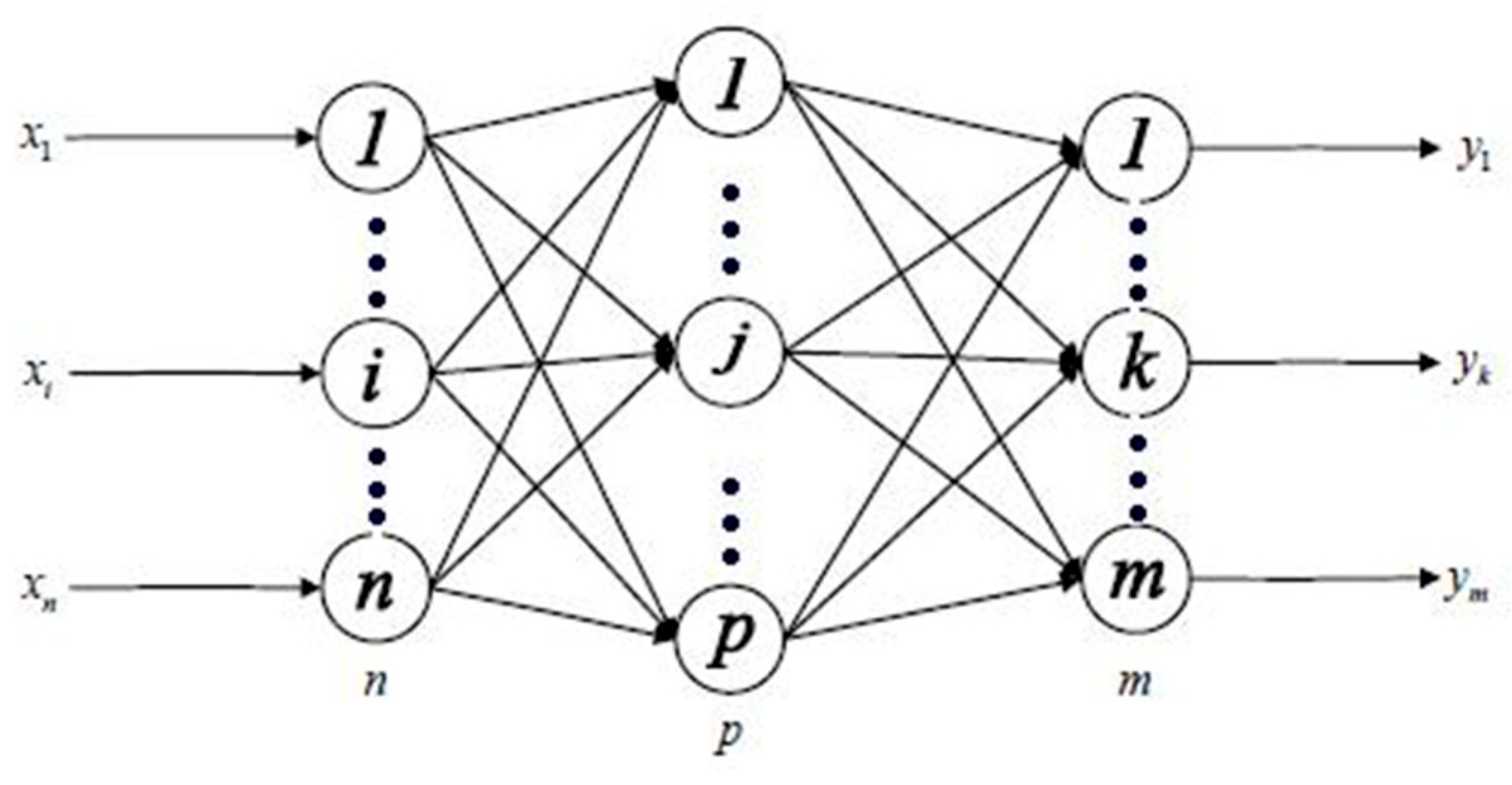
The BP artificial neural network is a layered structure consisting of an input layer, multiple hidden layers, and an output layer. Kolmogorov’s theorem has demonstrated that a single hidden layer with nodes having different thresholds can infinitely approximate any continuous function within a closed interval. Therefore, the three-layer BP neural network can accurately predict medium to long-term runoff by realizing any mapping from n-dimensions to m-dimensions. Information flows through this structure from the input layer and is processed by weight matrices and activation functions in the hidden layers before being transmitted level-by-level to the output layer for output. Figure 2 shows its network topology diagram.

In the figure, the input column vector of the network is $X={\left[x_1\cdot \cdot \cdot x_i\cdot \cdot \cdot x_n\right]}^{{\rm T}}$, and the output column vector is $Y={\left[y_1\cdot \cdot \cdot y_k\cdot \cdot \cdot y_m\right]}^{{\rm T}}$; n, p, m are the total number of nodes in the input layer, hidden layer, and output layer, respectively.

(2)

Network Learning Rules

The core operational process following the construction of a BP neural network can be divided into two stages: network learning (training) and association (prediction). Learning essentially involves clarifying the inherent connection between input and output network information. The BP algorithm is a supervised learning method, with training consisting of two steps. Firstly, forward transmission of information occurs where input flows through the hidden layer to obtain actual calculation values from the output layer. Secondly, backward correction of errors takes place by calculating discrepancies between actual calculated outputs and expected target values. When errors do not meet requirements, this serves as a basis for determining adjustment amounts for various parameters within the network while modifying weights and thresholds layer by layer. These two links complete an entire iteration process for network learning. After repeated iterations resulting in output error meeting accuracy requirements or reaching upper limits on training times, learning, and training cease.

2.

Problems and Improvements of BP Network

The BP artificial neural network is widely used and highly recognized. However, it also has limitation problems such as slow convergence speed, the tendency to get stuck in local minima, overfitting leading to poor generalization capabilities, and unclear principles for structure design. In response to these issues, the following improvements have been made to the BP network:

(1)

Adaptive Learning Rate $\eta$

The learning rate $\eta$ is a crucial parameter that impacts the speed of model convergence by adjusting the degree of correction for network errors. To enhance convergence and address the issue of reduced generalization caused by overtraining, it is necessary to appropriately adjust the learning rate based on specific circumstances. When utilizing BP networks to solve practical problems, determining whether to modify the learning rate value requires comparing the objective function values after each iteration with those from previous iterations. The adjustment value for the learning rate $\eta$ in l-th generation training can be expressed as follows:

$$\eta (l)=\left\{\begin{array}{cc}\eta (l-1)\hfill & \delta (l)<\delta (l-1)\hfill \\ e^{-\lambda }\eta (l-1)\hfill & \delta (l)\ge \delta (l-1)\hfill \end{array}\right.,$$

(2)

where $0.001\ge \lambda \ge 0.0001$, l is the number of training iterations, and $\delta$ is the measurement function, that is, the model error.

(2)

Correction of Weight Adjustment Amount

To make the training process of the BP network more stable, a momentum term is introduced to correct the weight adjustment amount, as shown in Equation 3.

$$\Delta w(l)=\eta \frac{\partial \delta }{\partial w}+\beta \Delta w(l-1),$$

(3)

where $\beta$ is the momentum term coefficient, $∆w$ is the weight adjustment amount, and other variables have the same meaning as above.

2.3.2. Factor Sensitivity Analysis Method

Various climatic factors have varying degrees of impact on medium-to-long-term runoff, and each factor exhibits different sensitivity to runoff prediction. This paper utilizes N significant factor set to establish a simulation prediction model for medium-to-long-term runoff based on an improved BP artificial neural network. By removing one factor at a time from the set, a new multi-factor simulation prediction model is established using the remaining N − 1 factors. The most sensitive factor is identified as the one that causes the greatest deterioration in simulation result error and fitting effect of the new model. Equation (4) defines sensitivity $\gamma$ to determine each influencing factor’s impact on medium-to-long-term runoff prediction.

$${\gamma }_i=\Delta {\epsilon }_i+\Delta {\varphi }_i,$$

(4)

where ${\gamma }_i$ is the sensitivity of the i-th factor in the significant factor set. The larger the sensitivity of the factor, the higher the sensitivity of the factor to medium-to-long-term runoff prediction. $\mathsf{\Delta }{\epsilon }_i$ is the increase in the average relative error of the model simulation after removing the i-th factor compared to before the removal (if it decreases, the increase value is negative). $\mathsf{\Delta }{\varphi }_i$ is the decrease in the Nash efficiency coefficient of the model simulation result after removing the i-th factor (if it increases, the decrease value is negative).

In order to further consider the impact of different data series’ lengths on the sensitivity ranking of each influencing factor, the existing n-year data series is divided into the first m years of the original data period and the later p years of the new data period. First, the factor sensitivity analysis is carried out with m years of original data, and the sensitivity ranking of each factor is obtained. Then, the p-year new data are divided into k equal parts, and the series length of the original data period is expanded k times. Each time the series length is increased, the factors are re-analyzed for sensitivity. Finally, the sensitivity ranking results of k + 1 times are compared. If the factors with significant sensitivity do not change, this multi-factor combination can be directly used for runoff prediction for a longer period in the future. If the factors with significant sensitivity change, when predicting future medium-to-long-term runoff, the data series needs to be continuously updated, and the factor sensitivity analysis needs to be carried out again before making runoff predictions.

2.4. Evaluation System for Prediction Results

2.4.1. Single Evaluation Index

To comprehensively evaluate the effects of the training period and validation period of each multi-factor combination scheme model, this article uses four commonly used indicators: Mean Absolute Relative Error (MARE), Nash Efficiency Coefficient (NSE), 20% standard forecast qualification rate ${\partial }_{20\%}$, and Standard Deviation of Relative Error $\sigma$.

1.

Mean Absolute Relative Error

$$MARE=\frac{1}{n}{\displaystyle \sum _{i=1}^n\left|\frac{Q\left(i\right)-Q_0\left(i\right)}{Q_0\left(i\right)}\right|},$$

(5)

where n is the total length of the sample series, $Q\left(i\right)$ is the runoff simulation value of the i-th sample, and $Q_0\left(i\right)$ is the actual runoff value of the i-th sample. When the runoff simulation value equals the actual value, the value of MARE is 0. Therefore, the closer it is to 0, the better the simulation effect.

2.

Nash Efficiency Coefficient

$$NSE=1-\frac{{\displaystyle \sum _{i=1}^n{\left(Q_0(i)-Q(i)\right)}^2}}{{\displaystyle \sum _{i=1}^n{\left(Q_0(i)-{\stackrel{-}{Q}}_0\right)}^2}},$$

(6)

where ${\stackrel{-}{Q}}_0$ is the average value of the actual runoff values of n samples, and the other variables have the same meaning as above. When NSE is 1, it means that the runoff simulation value equals the actual value, and the simulation effect is good. When NSE is 0, it means that the simulation result is approximately the average level of actual values, and the simulation effect is generally credible. When NSE is less than 0, the simulation effect is not credible. Therefore, the closer its value is to 1, the better the simulation effect of the model.

3.

20% Standard Forecast Qualification Rate

$${\partial }_{20\%}=\frac{n_h}{n},$$

(7)

where n is the total number of medium-to-long-term runoff predictions, and $n_h$ is the number of qualified predictions when the qualification rate standard is 20%. This indicator reflects the overall accuracy of the simulation, and the larger its value, the better the simulation effect.

4.

Standard Deviation of Relative Error

$${\partial }_{20\%}=\frac{n_h}{n},$$

(8)

In the formula, the variables have the same meaning as above. This indicator reflects the degree of deviation from the average value of the relative error distribution between the runoff simulation value and the actual value. The smaller the $\sigma$ value, the better the simulation effect.

2.4.2. Comprehensive Evaluation Index

When evaluating the pros and cons of the simulation effects of the training period and validation period of each multi-factor combination scheme model, different evaluation results may be produced based on different single indicators. Therefore, considering all single indicators, a comprehensive evaluation index is constructed to intuitively represent the pros and cons of the model simulation runoff effect.

Since each single evaluation index may have different dimensions and both high-quality indicators and low-quality indicators exist, they are not commensurable, so the initial index values cannot be used directly to determine the comprehensive evaluation index and need to be standardized and homogenized. If there are negative numbers in the index values, non-negativity processing is also required. After processing, this paper uses the entropy method that can objectively determine the weights of each single index to construct a comprehensive evaluation index. For an evaluation system of n schemes and m evaluation indexes, the specific calculation process is as follows:

1.

Calculation of Entropy

$$H_j=-k{\displaystyle \sum _{i=1}^n{f}_{ij}}\ln f_{ij}\hspace{1em}(j=1,2,\dots \dots ,m),$$

(9)

where $H_j$ is the entropy of the j-th evaluation index, $0\le H_j\le 1$; $k=\frac{1}{\mathit{ln}n}$; $f_{ij}=\frac{r_{ij}}{{\sum }_{i=1}^n{r}_{ij}}$; Among them $f_{ij}$ is the proportion of the j-th index of the i-th scheme in the index.

2.

Calculation of Entropy Weight

$${\omega }_j=\frac{1-H_j}{m-{\displaystyle \sum _{j=1}^m{H}_j}}(j=1,2,\dots \dots ,m),$$

(10)

where ${\omega }_j$ is the entropy weight of the j-th evaluation index, ${\sum }_{j=1}^m{\omega }_j=1 \mathrm{and} 0\le {\omega }_j\le 1$.

3. Results

3.1. Preliminary Selection of Factors

Using the monthly runoff process from January 1980 to December 2010 in a certain coastal area of Jiangsu, and the monthly climate index set from July 1979 to December 2010, the Spearman rank correlation coefficients of the monthly climate factors and the monthly runoff process of the forecast object at different lags were calculated according to Formula (1). Under the premise of a given confidence coefficient $\alpha =0.05$, the critical value $R_{\alpha }=0.297$. According to $\left|R_i\right|>R_{\alpha }$, the dominant factors that passed the significance test were initially selected from the 130 climate factors, as shown in Figure 3, Figure 4, Figure 5, Figure 6, Figure 7 and Figure 8. Among them, the number of early factors that passed the test at lags of 1–6 months were 29, 11, 16, 28, 36, and 33, respectively.

3.2. Construction of Significant Climate Factor Set

In order to find out all the factors that have a significant impact on runoff at different lags, the stepwise regression equation was established separately using the dominant factors in the first 1–6 months screened out by the Spearman rank correlation coefficient method and the monthly runoff process. Under the premise of a given confidence coefficient $\alpha =0.05$, factors that are independent of each other and have a significant impact on runoff at different lags were further selected. Considering these factors comprehensively, the significant climate factor set for medium and long-term runoff prediction in a certain coastal area of Jiangsu was constructed, as shown in

Table 2. Significant Climate Factor Set Affecting Medium and Long-term Runoff Prediction in a certain coastal area of Jiangsu.

Lag	Previous One Month	Previous Two Months	Previous Three Months	Previous Four Months	Previous Five Months	Previous Six Months
Factor Number	55	102	101	32	65	55
	66	101	104	101	58
	16	55	26	104	104
	102		31		101
	50

.

The above table reveals a total of 20 climate factors that have been carefully selected due to their significant impact on medium and long-term runoff during the first half of the year, at various time lags. Among these factors, there are five variables from the previous month, including the Northern Hemisphere Polar Vortex Strength Index, Tibet Plateau-au-2 Index, West Pacific Subtropical High Strength Index, Indian Ocean Warm Pool Strength Index, and Northern Hemisphere Polar Vortex Area Index. Additionally, there are 3 variables from two months prior: the Indian Ocean Warm Pool Strength Index, the Indian Ocean Warm Pool Area Index, and the Northern Hemisphere Polar Vortex Strength Index. Furthermore, there are four variables from three months ago: Indian Ocean Warm Pool Area Index; West Pacific Warm Pool Strength Index; India Subtropical High Ridge Line Position Inde. Moreover, there are three variables from four months earlier: North America-North Atlantic Subtropical High Ridge Line Position Index; Indian Ocean Warm Pool Area Index; and West Pacific Warm Pool Strength Index. In addition, there are four variables in the previous five months, including the Tibet Plateau-1 Index; the Northern Hemisphere Polar Vortex Center Strength Index; the West Pacific Warm Pool Strength Index; and the Indian Ocean Warm Pool Area Index. Finally, only one variable is considered from six months ago—the Northern Hemisphere Polar Vortex Strength Index.

Therefore, the formation of runoff in a certain coastal area of Jiangsu is closely related to factors such as the water vapor channel that affects precipitation, cold air moving southward, sea-air interaction, the dynamic and thermal effects of the Qinghai-Tibet Plateau, and teleconnection types. Among them, the West Pacific Subtropical High, the India Subtropical High, and the South China Sea Subtropical High control the water vapor transport channel, the polar vortex affects the southward cold air, the interaction between the West Pacific and Indian Ocean warm pools and the atmosphere affects the circulation situation, and the Tibet Plateau, through its unique dynamic and thermal effects of large terrain, the North America-North Atlantic Subtropical High is connected with the runoff in the study area through teleconnection.

3.3. Sensitivity Analysis Results

Using the 20 climate factors in the significant climate factor set affecting the medium and long-term runoff prediction in a certain coastal area of Jiangsu, and the local monthly runoff process from 1980 to 2010, a prediction model based on the improved BP artificial neural network was established. Using the sensitivity analysis method, the sensitivity of each factor in the significant factor set was obtained, and the sensitivity ranking of each factor is shown in

Table 3. Sensitivity Ranking of Each Factor in the Significant Factor Set.

Factor Number	Sensitivity	Ranking	Factor Number	Sensitivity	Ranking
102(1)	0.2936	1	101(4)	0.0379	11
55(6)	0.2617	2	102(2)	0.0330	12
50(1)	0.2187	3	31(3)	0.0321	13
16(1)	0.1635	4	58(5)	0.0305	14
101(2)	0.1216	5	66(1)	0.0213	15
101(5)	0.0866	6	104(5)	0.0205	16
26(3)	0.0842	7	104(4)	0.0201	17
101(3)	0.0831	8	32(4)	0.0173	18
65(5)	0.0508	9	55(2)	0.0147	19
104(3)	0.0407	10	55(1)	0.0083	20

Note: The numbers in parentheses represent the previous months, the same below.

.

As can be seen from Figure 9, the sensitivity values of the factors ranked in the top eight are significantly increased compared to the last 12 factors. This suggests that the climate factors ranking in the top eight are very sensitive to the medium and long-term prediction of runoff in the study area.

Considering the influence of data series length changes on the selection of significant sensitivity factors, further factor sensitivity analyses were conducted on the series from 1980 to 2000 and from 1980 to 2005, respectively. The results show that the factors ranked in the top eight in terms of sensitivity do not change with the length of the data series. This indicates that these eight factors have good temporal stability in terms of their sensitivity to runoff prediction in a certain coastal area of, Jiangsu, and can be used for runoff prediction in this area for a longer period of time in the future.

3.4. Multi-Factor Prediction Simulation Results of the Improved BP Neural Network Model

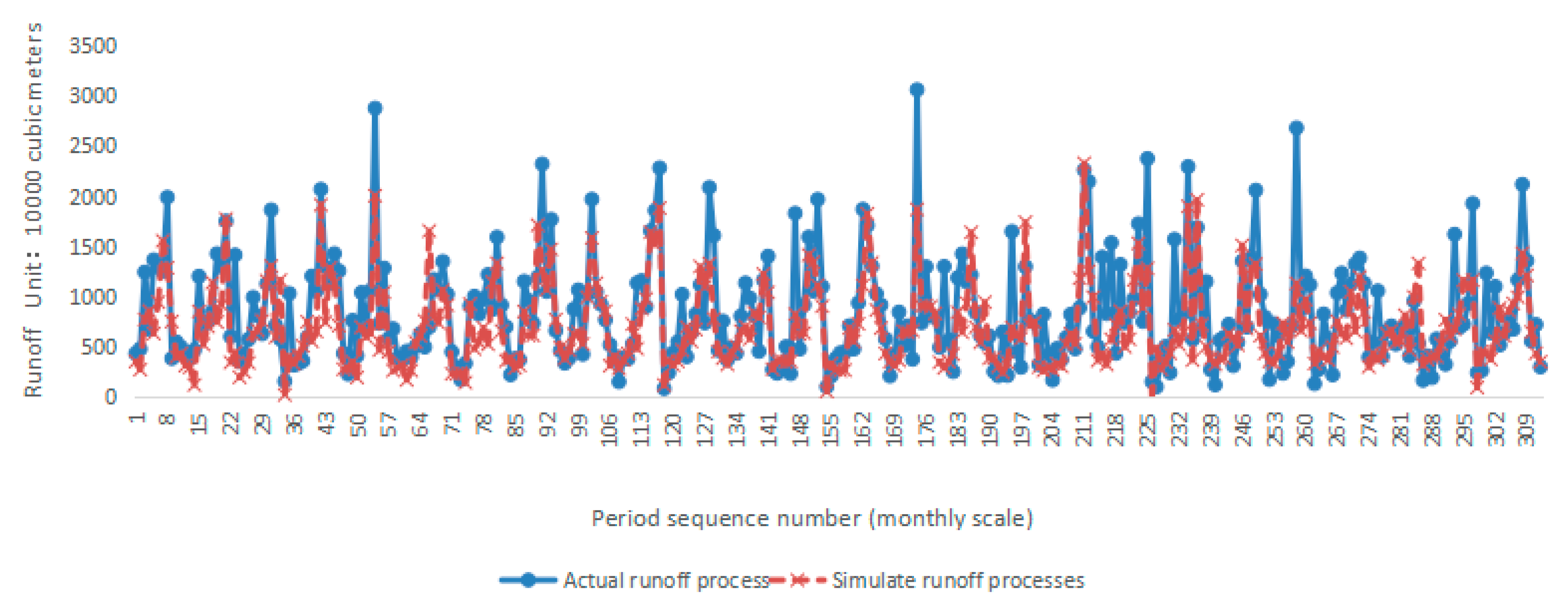
The actual monthly runoff process of the local area from 1980 to 2010 obtained from the hydrological monitoring station in a coastal area of Jiangsu Province was partitioned into a training period (1980–2005) and a validation period (2006–2010). With a given confidence coefficient, stepwise regression selected eight factors from the significant factor set. The top eight factors in the sensitivity ranking were highly sensitive and cannot be overlooked. Therefore, for multi-factor combination medium and long-term runoff simulation prediction in the study area, eight factors were chosen. An improved BP neural network model based on sensitivity analysis was utilized for simulation prediction, as shown in Figure 10 and Figure 11 for the training and validation periods, respectively. It can be seen that the improved BP neural network model based on multi-factor sensitivity analysis constructed in this study can better reflect the measured runoff law in the simulated runoff process during the training and validation periods, effectively extending the prediction period of runoff forecasting, predicting the future runoff variation law through changes in atmospheric weather systems in advance, and providing a basic reference for clarifying the physical causes of runoff formation and variation in the coastal areas of Jiangsu Province from the perspective of atmospheric circulation, as well as establishing a medium- and long-term runoff forecasting model.

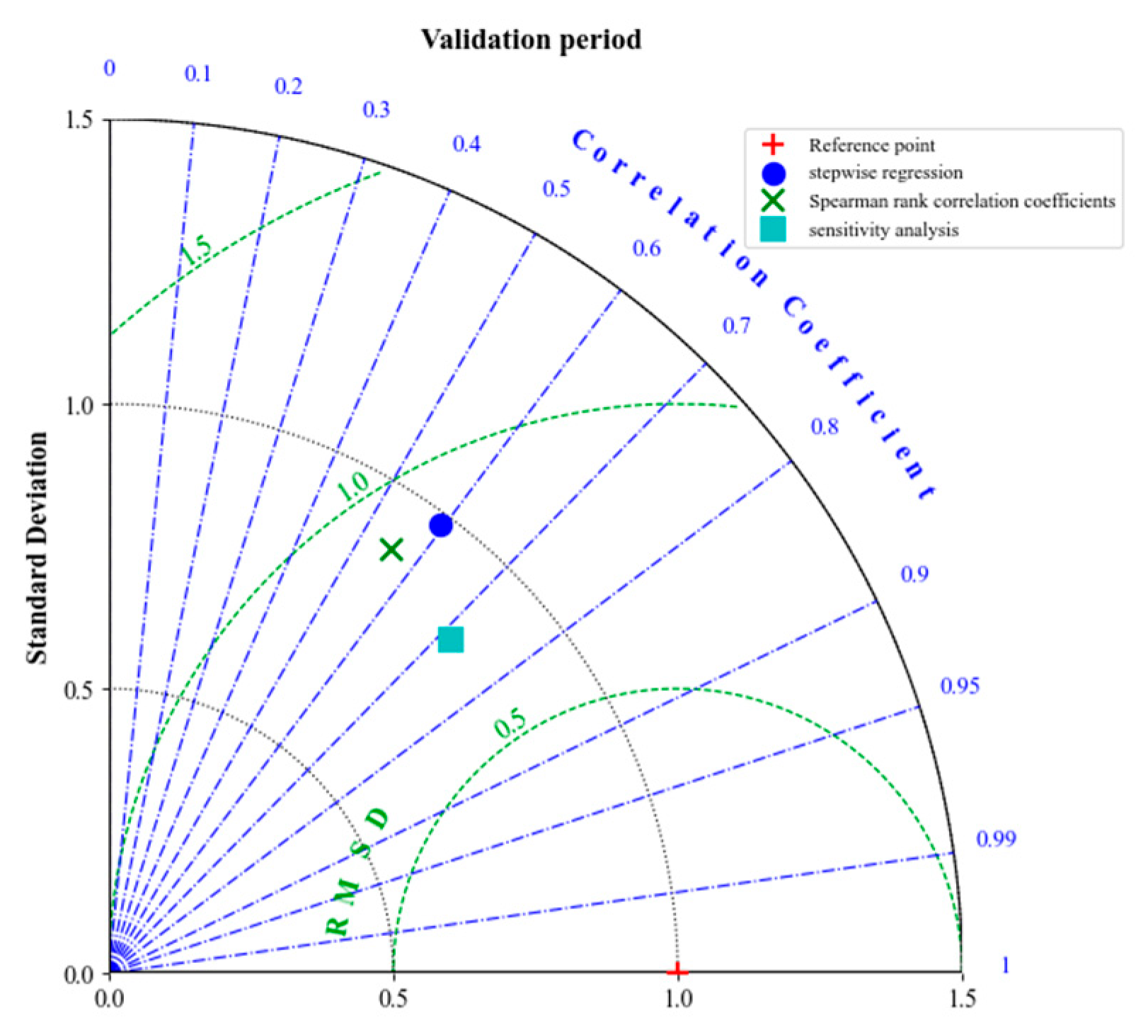
As shown in Figure 12 and Figure 13, from the Taylor diagram of the prediction results, it can be seen that the correlation coefficient of the model based on sensitivity analysis is between 0.7 and 0.8. In the simulation prediction results during the validation period, the model’s centered root mean square error significantly decreased, showing better simulation prediction performance overall compared to the other two models.

4. Discussion

4.1. Comparison of Simulation Accuracy for Different Factor Quantities

In order to further validate the reasonability and reliability of the selected factors for multi-factor combination runoff simulation prediction in the study area, we trained and built models using the top 9 and top 10 factors from the sensitivity analysis method (1980–2005). Subsequently, we compared the Mean Squared Error (MSE) and Nash-Sutcliffe Efficiency (NSE) indexes of the prediction results during the validation period (2006–2010) with those obtained from a model utilizing only the top eight factors. As shown in

Table 4. Comparison of prediction effects of different factor quantity models.

Selection Factor	Factor Number	MARE	NSE
the first 8 factors	102(1), 55(6), 50(1), 16(1), 101(2), 101(5), 26(3), 101(3)	0.3800	0.45
the first 9 factors	102(1), 55(6), 50(1), 16(1), 101(2), 101(5), 26(3), 101(3), 65(5)	0.3783	0.47
the first 10 factors	102(1), 55(6), 50(1), 16(1), 101(2), 101(5), 26(3), 101(3), 65(5), 104(3)	0.3770	0.50

, increasing the number of influencing factors from 8 to 10 resulted in a marginal decrease of only 0.003 in the MSE index and an increase of merely 0.05 in the NSE index, indicating limited improvement in prediction accuracy. Therefore, considering this limitation, we controlled as much as possible by inputting a reduced number of influencing factors into our model to enhance its learning efficiency while ensuring that our selection for simulation prediction was reasonable and reliable.

4.2. Simulation Comparison of Three Multiple Factor Combination Schemes

In this study, the widely used and highly recognized improved BP artificial neural network model is employed. Three different multi-factor combination medium and long-term runoff prediction schemes are constructed based on variance contribution, rank correlation coefficient, and sensitivity value indicators combined with stepwise regression, Spearman rank correlation, and sensitivity analysis. The evaluation index system’s advantages and disadvantages in each combination scheme’s training period and validation period are comparatively analyzed. Additionally, the sensitivity analysis factor selection method’s strengths and weaknesses are evaluated. Ultimately, eight factors are selected using stepwise regression, Spearman rank correlation, and sensitivity analysis as shown in

Table 5. Different multi factor combination schemes.

Screening Method	Stepwise Regression	Spearman Related	Sensitivity Analysis
Factor Number	55(6)	55(6)	102(1)
	32(4)	32(4)	55(6)
	55(2)	58(5)	50(1)
	101(5)	65(5)	16(1)
	66(1)	101(4)	101(2)
	16(1)	101(3)	101(5)
	50(1)	16(1)	26(3)
	102(1)	55(1)	101(3)

.

The BP artificial neural network model is trained 30,000 times with eight hidden layer nodes determined by trial calculation. The initial learning rate and allowable error of the initial network are set accordingly. Three multi-factor combination schemes selected by stepwise regression, Spearman rank correlation, and sensitivity analysis are assumed to be schemes one, two, and three, respectively. These three schemes utilize the improved BP artificial neural network model to simulate medium- and long-term runoff in the study area while calculating single indicator values during both training and validation periods as shown in

Table 6. The values of each individual indicator during the training period of three schemes.

	MARE (%)	NSE	∂20% (%)	σ
Scheme 1	37.67	0.60	37.82	0.41
Scheme 2	48.47	0.66	37.50	0.70
Scheme 3	36.61	0.51	33.01	0.34

and

Table 7. Value of each individual indicator during the validation period of three schemes.

	MARE (%)	NSE	∂20% (%)	σ
Scheme 1	43.87	0.21	36.67	0.39
Scheme 2	50.26	0.19	30.00	0.50
Scheme 3	38.01	0.45	31.67	0.27

. Low-optimal type indicators within the evaluation index system are uniformly converted into high-optimal type indicators before normalization takes place. Comprehensive evaluation index values of each scheme are then calculated using the entropy method where higher values indicate better simulation effects of the model. Entropy weights along with comprehensive index values for each evaluation index can be found in

Table 8. Entropy weight of each evaluation index.

	MARE (%)	NSE	∂20% (%)	σ
Training period	0.0686	0.0900	0.0306	0.8107
Validation period	0.0400	0.8140	0.0368	0.1092

and

Table 9. Comprehensive indicator values for the training and validation periods of three schemes.

	Scheme 1	Scheme 2	Scheme 3
Training period	0.583	0.349	0.636
Validation period	0.273	0.241	0.482

.

The comparison of the three schemes reveals that Scheme Three exhibits the smallest average relative error in both training and validation periods, while its Nash efficiency coefficient is relatively poor during the rating period but significantly better than Schemes One and Two in the validation period, indicating superior generalization ability. Moreover, all three schemes demonstrate similar 20% standard forecast pass rates. Notably, Scheme Three displays a much smaller standard deviation of relative error in both training and validation periods compared to Schemes One and Two, suggesting minimal dispersion of its relative error. Overall, considering these four single indicators comprehensively during both rating and validation periods using objective weighting entropy method yields Scheme Three as having the best comprehensive evaluation index with optimal simulation effect.

4.3. Research Characteristics and Prospects

The multi-factor combination medium and long-term runoff prediction model developed in this study, based on an improved BP neural network, exhibits several innovative features. However, it also possesses certain methodological limitations and deficiencies identified in existing literature, studies that require further investigation. These limitations primarily pertain to the following aspects.

(1) This study focuses more on studying and analyzing the impact of changes in meteorological and hydrological factors in the early stages on runoff changes over a longer period of time and analyzing the impact of multi-factor combinations under different screening criteria on runoff prediction. However, it does not combine different models or use combined models to analyze the impact on runoff prediction accuracy.

(2) this study seeks to optimize a small number of physical factors with significant impacts from a large number of climate impact factors, and on the basis of meeting the requirements of prediction accuracy, minimize model input factors, simplify model network structure, reduce network training burden, and improve model learning efficiency. However, it does not further analyze the prediction effect of large-scale weather system characteristic factors themselves on runoff processes under different human activity disturbances.

(3) although this study considered the different effects of various pre-event meteorological and hydrological factors on the formation of runoff processes under different lag times when selecting significant factors, it did not analyze and compare the prediction effects of relevant factors during the flood season and non-flood season on the runoff process.

5. Conclusions

The prediction of medium and long-term runoff holds significant importance for the coordinated management of water resources. This study focuses on evaluating the impact of different multi-factor combinations, selected through various methods, on the prediction accuracy of medium and long-term runoff in a specific coastal area of Jiangsu. The analysis is based on the latest monthly index set comprising 130 climate systems released by the National Climate Center. Consequently, this research has yielded the following outcomes:

(1) Using the Spearman rank correlation coefficient, 29, 11, 16, 28, 36, and 33 dominant climate factors were identified for medium to long-term runoff prediction in the coastal area of Jiangsu over a period of one to six months.

(2) Through stepwise regression analysis, a set of 20 significant climate factors with good independence at different lag times was selected for further analysis.

(3) According to the stepwise regression, Spearman rank correlation, and sensitivity analysis methods, a total of eight factors were selected from the significant factor set individually, resulting in three distinct multi-factor combination schemes. Utilizing an improved BP artificial neural network for simulating medium and long-term runoff in the research area, a comparison of comprehensive evaluation index values between the three schemes during both the rating period and verification period revealed that the sensitivity analysis method yielded the most effective simulation results. The comprehensive index values for this scheme were 0.636 and 0.482, respectively, during the training period and verification period. Furthermore, it was observed that these selected eight factors exhibited relatively stable sensitivities over time. Therefore, this particular multi-factor combination is chosen for predicting medium and long-term runoff in coastal areas of Jiangsu province.

The eight climate factors include the Indian Ocean Warm Pool Intensity Index, the Northern Hemisphere Vortex Area Index, and the Western Pacific Subtropical High Intensity Index from the previous month. Additionally, it comprises the Indian Ocean Warm Pool Area Index from the previous two months, the Indian Subtropical High Ridge Line Position Index, and the Indian Ocean Warm Pool Area Index from the previous three months. Furthermore, it incorporates the Indian Ocean Warm Pool Area Index from the previous five months and finally concludes with the Northern Hemisphere Vortex Intensity Index from the previous six months.

(4) The method optimizes eight pre-climate indexes suitable for the coastal area of Jiangsu Province. In the future, these optimized pre-significant factors can be directly utilized for regional runoff prediction, providing a valuable reference for formulating flood control and relief strategies, farmland irrigation management, hydropower station operations, and other disaster relief scheduling plans in the region. Moreover, this approach introduces novel perspectives for medium and long-term runoff forecasting in the region.

References

1. Korsic, S.A.T.; Notarnicola, C.; Quirno, M.U.; Cara, L. Assessing a data-driven approach for monthly runoff prediction in a mountain basin of the Central Andes of Argentina. Environ. Chall. 2023, 10, 100680. [Google Scholar] [CrossRef]
2. Yu, Y.; Hua, T.; Chen, L.; Zhang, Z.; Pereira, P. Divergent Changes in Vegetation Greenness, Productivity, and Rainfall Use Efficiency Are Characteristic of Ecological Restoration Towards High-Quality Development in the Yellow River Basin, China. Engineering 2023, in press. [Google Scholar] [CrossRef]
3. Yu, Y.; Feng, J.; Liu, H.; Wu, C.; Zhang, J.; Wang, Z.; Liu, C.; Zhao, J.; Rodrigo-Comino, J. Linking hydrological connectivity to sustainable watershed management in the Loess Plateau of China. Curr. Opin. Environ. Sci. Health 2023, 35, 100493. [Google Scholar] [CrossRef]
4. Hatta, S.; Nishimura, T.; Saga, H.; Fujita, M. Study on snowmelt runoff prediction using weekly weather forecast. Environ. Int. 1995, 21, 501–507. [Google Scholar] [CrossRef]
5. Aizen, V.; Aizen, E.; Glazirin, G.; Loaiciga, H.A. Simulation of daily runoff in Central Asian alpine watersheds. J. Hydrol. 2000, 238, 15–34. [Google Scholar] [CrossRef]
6. Trivedi, H.V.; Singh, J.K. Application of Grey System Theory in the Development of a Runoff Prediction Model. Biosyst. Eng. 2005, 92, 521–526. [Google Scholar] [CrossRef]
7. Gusev, E.M.; Nasonova, O.N.; Dzhogan, L.Y. Reproduction of Pechora runoff hydrographs with the help of a model of heat and water exchange between the land surface and the atmosphere (SWAP). Water Resour. 2010, 37, 182–193. [Google Scholar] [CrossRef]
8. Yu, Y.; Zhu, R.; Ma, D.; Liu, D.; Liu, Y.; Gao, Z.; Yin, M.; Bandala, E.R.; Rodrigo-Comino, J. Multiple surface runoff and soil loss responses by sandstone morphologies to land-use and precipitation regimes changes in the Loess Plateau, China. Catena 2022, 217, 106477. [Google Scholar] [CrossRef]
9. Rai, R.K.; Upadhyay, A.; Singh, V.P. Effect of variable roughness on runoff. J. Hydrol. 2010, 382, 115–127. [Google Scholar] [CrossRef]
10. Samantaray, S.; Sawan Das, S.; Sahoo, A.; Prakash Satapathy, D. Monthly runoff prediction at Baitarani river basin by support vector machine based on Salp swarm algorithm. Ain Shams Eng. J. 2022, 13, 101732. [Google Scholar] [CrossRef]
11. Di Nunno, F.; de Marinis, G.; Granata, F. Short-term forecasts of streamflow in the UK based on a novel hybrid artificial intelligence algorithm. Sci. Rep. 2023, 13, 7036. [Google Scholar] [CrossRef] [PubMed]
12. Song, C.M. Data construction methodology for convolution neural network based daily runoff prediction and assessment of its applicability. J. Hydrol. 2022, 605, 127324. [Google Scholar] [CrossRef]
13. Cheng, Z.; Liu, Y.; Gao, C.; Hu, J.; Cui, T. Long-term runoff prediction for reservoir based on Mahalanobis distance discrimination. In Proceedings of the MATEC Web of Conferences, Beijing, China, 16–20 October 2018; p. 02028. [Google Scholar]
14. Crochemore, L.; Ramos, M.-H.; Pappenberger, F. Bias correcting precipitation forecasts to improve the skill of seasonal streamflow forecasts. Hydrol. Earth Syst. Sci. 2016, 20, 3601–3618. [Google Scholar] [CrossRef]
15. Yuan, X.; Ma, F.; Wang, L.; Zheng, Z.; Ma, Z.; Ye, A.; Peng, S. An experimental seasonal hydrological forecasting system over the Yellow River basin–Part 1: Understanding the role of initial hydrological conditions. Hydrol. Earth Syst. Sci. 2016, 20, 2437–2451. [Google Scholar] [CrossRef]
16. Wang, W.-c.; Chau, K.-w.; Qiu, L.; Chen, Y.-b. Improving forecasting accuracy of medium and long-term runoff using artificial neural network based on EEMD decomposition. Environ. Res. 2015, 139, 46–54. [Google Scholar] [CrossRef] [PubMed]
17. Bray, M.; Han, D. Identification of support vector machines for runoff modelling. J. Hydroinform. 2004, 6, 265–280. [Google Scholar] [CrossRef]
18. Nourani, V.; Tajbakhsh, A.D.; Molajou, A. Data mining based on wavelet and decision tree for rainfall-runoff simulation. Hydrol. Res. 2019, 50, 75–84. [Google Scholar] [CrossRef]
19. Borne, M.; Lorenz, C.; Portele, T.C.; Martins, E.S.P.R.; Vasconcelos Junior, F.d.C.; Kunstmann, H. Seasonal sub-basin-scale runoff predictions: A regional hydrometeorological Ensemble Kalman Filter framework using global datasets. J. Hydrol. Reg. Stud. 2022, 42, 101146. [Google Scholar] [CrossRef]
20. Lee, E.H. Runoff prediction of urban stream based on the discharge of pump stations using improved multi-layer perceptron applying new optimizers combined with a harmony search. J. Hydrol. 2022, 615, 128708. [Google Scholar] [CrossRef]
21. Shoaib, M.; Shamseldin, A.Y.; Melville, B.W. Comparative study of different wavelet based neural network models for rainfall–runoff modeling. J. Hydrol. 2014, 515, 47–58. [Google Scholar] [CrossRef]
22. Asadi, S.; Shahrabi, J.; Abbaszadeh, P.; Tabanmehr, S. A new hybrid artificial neural networks for rainfall–runoff process modeling. Neurocomputing 2013, 121, 470–480. [Google Scholar] [CrossRef]
23. Guo, J.; Liu, Y.; Zou, Q.; Ye, L.; Zhu, S.; Zhang, H. Study on optimization and combination strategy of multiple daily runoff prediction models coupled with physical mechanism and LSTM. J. Hydrol. 2023, 624, 129969. [Google Scholar] [CrossRef]
24. Granata, F.; Di Nunno, F. Neuroforecasting of daily streamflows in the UK for short-and medium-term horizons: A novel insight. J. Hydrol. 2023, 624, 129888. [Google Scholar] [CrossRef]
25. Kumar, V.; Kedam, N.; Sharma, K.V.; Mehta, D.J.; Caloiero, T. Advanced Machine Learning Techniques to Improve Hydrological Prediction: A Comparative Analysis of Streamflow Prediction Models. Water 2023, 15, 2572. [Google Scholar] [CrossRef]
26. Tokar, A.S.; Johnson, P.A. Rainfall-runoff modeling using artificial neural networks. J. Hydrol. Eng. 1999, 4, 232–239. [Google Scholar] [CrossRef]
27. Vidyarthi, V.K.; Jain, A.; Chourasiya, S. Modeling rainfall-runoff process using artificial neural network with emphasis on parameter sensitivity. Model. Earth Syst. Environ. 2020, 6, 2177–2188. [Google Scholar] [CrossRef]
28. Ju, Q.; Yu, Z.; Hao, Z.; Ou, G.; Zhao, J.; Liu, D. Division-based rainfall-runoff simulations with BP neural networks and Xinanjiang model. Neurocomputing 2009, 72, 2873–2883. [Google Scholar] [CrossRef]
29. Jain, A.; Srinivasulu, S. Development of effective and efficient rainfall-runoff models using integration of deterministic, real-coded genetic algorithms and artificial neural network techniques. Water Resour. Res. 2004, 40, W04302. [Google Scholar] [CrossRef]
30. Li, M.; Liu, W.; Fu, Q.; Liu, D.; Li, T.; Xu, Y.; Shang, R. Multi-layer multi-objective cooperative regulation of agricultural water resources in large agricultural irrigation areas based on runoff prediction. Comput. Electron. Agric. 2023, 208, 107761. [Google Scholar] [CrossRef]
31. Qiao, X.; Peng, T.; Sun, N.; Zhang, C.; Liu, Q.; Zhang, Y.; Wang, Y.; Shahzad Nazir, M. Metaheuristic evolutionary deep learning model based on temporal convolutional network, improved aquila optimizer and random forest for rainfall-runoff simulation and multi-step runoff prediction. Expert Syst. Appl. 2023, 229, 120616. [Google Scholar] [CrossRef]
Figure 1. Spatial distribution map of Jiangsu coastal area.
Water 15 03559 g001
Figure 2. Schematic Diagram of Three-layer BP Artificial Neural Network Structure.
Water 15 03559 g002
Figure 3. Primary chart of dominant factors a month ago.
Water 15 03559 g003
Figure 4. Primary chart of dominant factors two months ago.
Water 15 03559 g004
Figure 5. Primary chart of dominant factors three months ago.
Water 15 03559 g005
Figure 6. Primary chart of dominant factors four months ago.
Water 15 03559 g006
Figure 7. Primary chart of dominant factors five months ago.
Water 15 03559 g007
Figure 8. Primary chart of dominant factors six months ago.
Water 15 03559 g008
Figure 9. Sensitivity of each factor in the set of significant factors.
Water 15 03559 g009
Figure 10. Runoff simulation process during training period.
Water 15 03559 g010
Figure 11. Runoff simulation process during validation period.
Water 15 03559 g011
Figure 12. Taylor diagram of runoff prediction results during training period.
Water 15 03559 g012
Figure 13. Taylor diagram of runoff prediction results during validation period.
Water 15 03559 g013