1. Introduction
The uneven distribution of urban water resources is not coordinated with land resources, and there are many areas where groundwater levels drop and rivers dry up, which may further lead to a shortage of national water resources and have extremely adverse effects on social development [
1]. Therefore, there is an urgent need to address the issues of water resource waste and pollution at this stage, and to strengthen water resource protection. The protection of water resources involves both source control and the absorption and treatment of water pollutants. There are many ways to treat pollutants in water, and building absorption and utilization methods is one of the solutions. However, there are many studies on the removal of pollutants from water through plant absorption and other methods [
2], with few studies on building absorption. Buildings are important components of a city, and if they can effectively absorb pollutants from water, they are of great significance for the sustainable development of the city.
A concrete structure is the most used form of infrastructure and civil buildings. It is beneficial for its durability, very high strength, low cost, and easy availability [
3,
4,
5,
6,
7,
8,
9,
10]. Concrete can absorb wastewater, and the absorption of various ions in wastewater has a certain impact on the mechanical properties and durability of materials. The degree of influence is determined by factors such as the type and total amount of ions [
11]. Concrete absorbs important pollutants in water, such as sulfate ions, which can cause complex physical and chemical reactions, thereby affecting bearing capacity and sustainability. Sulfate ions form soluble gypsum through chemical and physical interactions with hardened cement paste, and then generate ettringite [
7]. These corrosion products will fill the pores of the concrete, thereby enhancing the bearing capacity and sustainability of concrete in the early stages. Due to the lengthy process of making concrete that has lasted for decades, the gradually generated expansion stress in the later stage of the concrete making process will also cause a decrease in strength, leading to building problems. Therefore, the performance of this process is predicted to understand whether the absorption of water pollutants has a positive or negative impact on buildings [
12,
13]. A successful prediction can avoid absorbing pollutants in water while reducing the bearing capacity in architectural design, thereby achieving the absorption and reuse of water pollutants. The final change rate of compressive strength (CSR) of concrete material is one of the important points of the carrying capacity and sustainability of buildings [
14,
15,
16]. Traditional methods usually study concrete strength data through a large number of laboratory tests, and some laboratory data and engineering detection data have been accumulated [
17,
18,
19,
20,
21,
22]. At present, the current research mostly used the mathematical method of statistical regression to obtain the performance change curve by fitting the experimental data [
8,
23,
24,
25]. The functional relationships used in the fitting were different, and usually only one was obtained. Nevertheless, the achievements of these regression methods are chiefly the size, quality, and reliability of the used experimental data, as well as the chosen function [
26]. Milad et al. [
27] summarized the processes and drawbacks of the basic mathematical regression formula and expert experience method. These methods are universal and can be used in various disciplines. Nevertheless, it is obvious that the complex nonlinear problem predicting the CSR of concrete under sulfate corrosion does not apply to these methods, because it cannot be expressed by one or several formulas due to many factors affecting the CSR. Because there are some defects in empirical methods, it seems that more advanced tools for analyzing complex nonlinear problems should be considered, which can reduce the number of laboratory tests and overcome the defects of traditional methods. This new method can better predict CSR at the same time.
To these aims, the use of progressive methods is needed to establish evaluation relationships. Recently, researchers used machine learning methods to investigate the compressive strength of concrete, e.g., artificial neural networks (ANNs) [
28], ensemble learning [
29], adaptive neuro-fuzzy inference systems and gene expression programming [
30], and gray correlation analysis [
31]. There is a common feature in these studies, which is the use of multiple machine learning models integrated together so as to prevent the limitations of evaluation results, such as low accuracy and generalization. Nevertheless, the method is only effective for specific problems and is not conducive to engineering popularization. Obviously, the CSR of a concrete structure under sulfate corrosion in a real service environment is worth studying. Sahoo et al. [
32] studied a double-hidden-layer back propagation ANN to estimate the compressive strength of concrete against sulfate corrosion. The input parameters included sulfate exposure periods, water curing days, and different ratios of fly ash replacement to binder. And 162 cubes were applied to train the ANN algorithm employing EXCEL of MS OFFICE. They only studied fly ash concrete, the corresponding scope of application was narrow, and the data and software were limited. Admixtures are indeed helpful to improve the sulfate resistance of concrete, but this is only one of the factors affecting the CSR. The factors should be studied together and should not be separated. Therefore, deep learning (DL) methods that can solve this problem appear. The basis of DL is a series of new structures and methods evolved in order to make an ANN with more layers that can be trained and run. DL has a priori knowledge about the physical world that cannot be obtained from the rigor of mathematics compared to ordinary ANN [
33]. It has more advantages in practical engineering problems, because like biological learning, it is used to find the ‘physical relationship’ that increases entropy. The learning goal is not simply to reduce the loss function. In addition, a shallow ANN can simulate any function, but the cost of the data volume is unacceptable. The amount of data in the field of concrete engineering is not as much as commercial data. Fortunately, DL solves this problem and can learn better fitting with less data compared with shallow ANN. Moreover, the TensorFlow (TF) method has been used for DL and has achieved significant performance and power-saving improvements.
With the consideration the above points, this paper implements a DL algorithm based on the TF framework to estimate the CSR of concrete under sulfate corrosion, which is necessary for the carrying capacity and sustainability of buildings. The aim of this paper is to construct a detailed configured DL model that can evaluate the CSR of concrete and ensure an ample applicability. The capability of this model is investigated, and the predicted results are visualized. Moreover, to verify the performance of the model, seven typical machine learning approaches will be applied to simulate the experiment, and the results will be compared with the DL model. The rest of this paper is formulated as follows.
Section 1 introduces the comprehensive structure of the proposed DL model and introduces the detailed approach.
Section 2 gives all the dataset generation and the correlation analysis processes.
Section 3 shows the results of the testing and training, discusses the development, performance, and interpretation of the model, and compares the proposed method with seven basic machine learning algorithms. Finally, the conclusions and future works are discussed in
Section 4.
2. Data and Methods
2.1. Methodologies
TensorFlow (TF) is an open-source and commutative program software library for machine learning (ML), proposed by the Google Brain Team, and it can be applied to compute information to evaluate the accuracy output. Version 2.0 was released in March 2019, and it was used in this study. As the name TF implies, operations are performed by DL on multidimensional data arrays. TF offers various popularly applied and powerful DL algorithms. TF applies dataflow graphs to represent the shared state, computation, and the operations that mutate that state [
34].
ANN is the basis of DL and is scalable, powerful, and versatile. DL is a subfield of ML that is a series of algorithms. At present, most ANNs are shallow structure algorithms, and the representation ability of complex functions is limited in the case of limited samples and calculation units. Therefore, for complex problems, the generalization ability is restricted to some extent. DL can realize complex function approximation by learning a deep nonlinear network structure, it can characterize the distributed representation of input data, and shows a strong ability to learn data and essential characteristics from a small number of samples. The advantage of a multilayer is that complex functions can be represented with fewer parameters. The essence of DL is to learn more useful features by building ML models with many hidden layers and massive training data so as to finally improve the accuracy of prediction. Therefore, a depth model is the means and feature learning is the purpose. Different from traditional shallow learning, DL is characterized by the following: (1) it emphasizes the depth of the model structure, which usually exceeds the hidden layer of two layers, and (2) it clearly highlights the importance of feature learning. Through layer-by-layer feature transformation, the feature representation of the sample in the original space is transformed into a new feature space, which makes the prediction easier. Compared with the method of constructing features using artificial rules, using big data to learn features can better describe the rich internal information of the data. The connection between neurons is shown by the straight line. DL is very similar to the ANN. In short, an ANN with two or more hidden layers is called a DL model. Combined with the TF framework, the model is mainly composed of the following parts:
Layers: They contain input, hidden, and output layers. The full connection layer was used in this paper. Each node was connected with all nodes of the previous layer, which was used to synthesize the previously extracted features.
Loss function: It is used to define the error between a single training sample and the real value. In the process of training, the weight needs to be constantly adjusted. Its purpose is to obtain a set of final weights to make the output of the input characteristic data reach the expected value.
Optimizer: The principal function of the optimizer is to guide the parameters of the loss function to update the appropriate size in the correct direction in the process of back propagation, so that the updated value continues to approach the global minimum.
Activation function: In the model, the input features act on the activation function after a series of weighted summation. Similar to the neuron-based model in the human brain, the activation function ultimately determines whether to transmit the signal and what to transmit to the next neuron. However, it is not the function with excellent characteristics that is the most suitable. Each function needs to be tested continuously in the model so that the most suitable function is selected. The swish function proved to be the most suitable activation function for the model after many experiments, which has several characteristics: (1) it is unbounded above (avoids saturation), (2) bounded below (strong regularization, especially for large negative numbers), (3) and smooth (accessible to learn and less sensitive to it). The swish function is represented as
Overfitting: The model performs too well in the training set, resulting in poor performance in the validation data and testing data, that is, the generalization error is relatively large. From the perspective of variance and deviation, overfitting means high variance and low deviation on the training set. Overfitting is usually caused by an amount of data that is too small, inconsistent data distribution between the training set and validation set, model complexity that is too large, poor data quality, overtraining, and so on. In order to reduce the complexity of the model, the regularization method was used in this paper. There are two regularization methods,
L1 and
L2:
where
represents the penalty number (regularization rate), and
presents weight value.
L2 has some advantages: a unique solution, more convenient calculation, better effect of preventing overfitting, and making the optimizer solver more stable and faster. Therefore,
L2 was chosen for this model.
If there are too few samples, the iterative calculation can be carried out in the form of full-batch learning, which has two advantages: (1) the direction decided by the complete data can represent the overall samples well; (2) it is difficult to choose a global learning rate due to the various gradient values of various weights. However, the above two advantages become disadvantages for a slightly larger dataset. It becomes infeasible to load all the data at one time, and the gradient correction values will offset each other because of sampling divergences between batches, and they cannot be corrected when iterated by the Rprop algorithm. Therefore, this model selected the mini-batch learning technique to promote the parallelization efficiency of matrix multiplication and decrease the loss value of the model. In addition, this model selected the exponential decay method to update the learning rate for the convergence speed because this update method is fast, and it selected the exponential moving average method to update the weight because it can make the model become more robust.
where the shadow variable is maintained for each variable. The initial value of the shadow variable is the initial value of the corresponding variable, and decay represents the exponential moving average decay rate.
2.2. Data and Preparation
The preparation of data is very important for the establishment of the model. The quality/quantity and division of dataset have a great impact on the results. The data of this study were from 148 sources in the literature, with a total of 1328 groups of data (
https://www.zotero.org/groups/5162364/water-15-03152-data/library). Obviously, the data sources were relatively extensive. Even if individual data results were inappropriate, they would not affect the final prediction results. This was of great benefit to the generalization of the model because the ultimate purpose of this study is to use the model in engineering practice, and the data in actual engineering cannot be as accurate as that in the laboratory. According to the composition of data and expert experience, six input parameters were selected: (1) water-to-binder ratio (W/B), (2) sulfate concentration (SC), (3) sulfate type (ST), (4) admixture type (AT), (5) admixture percentage in relation to the total binder (A/B), and (6) service age (SA). The output training vector’s output parameter has a dimension of
and consists of the final change rate of compressive strength (CSR).
Table 1 shows the range, mean and standard deviation (STD) values, and the regression coefficient of the parameters.
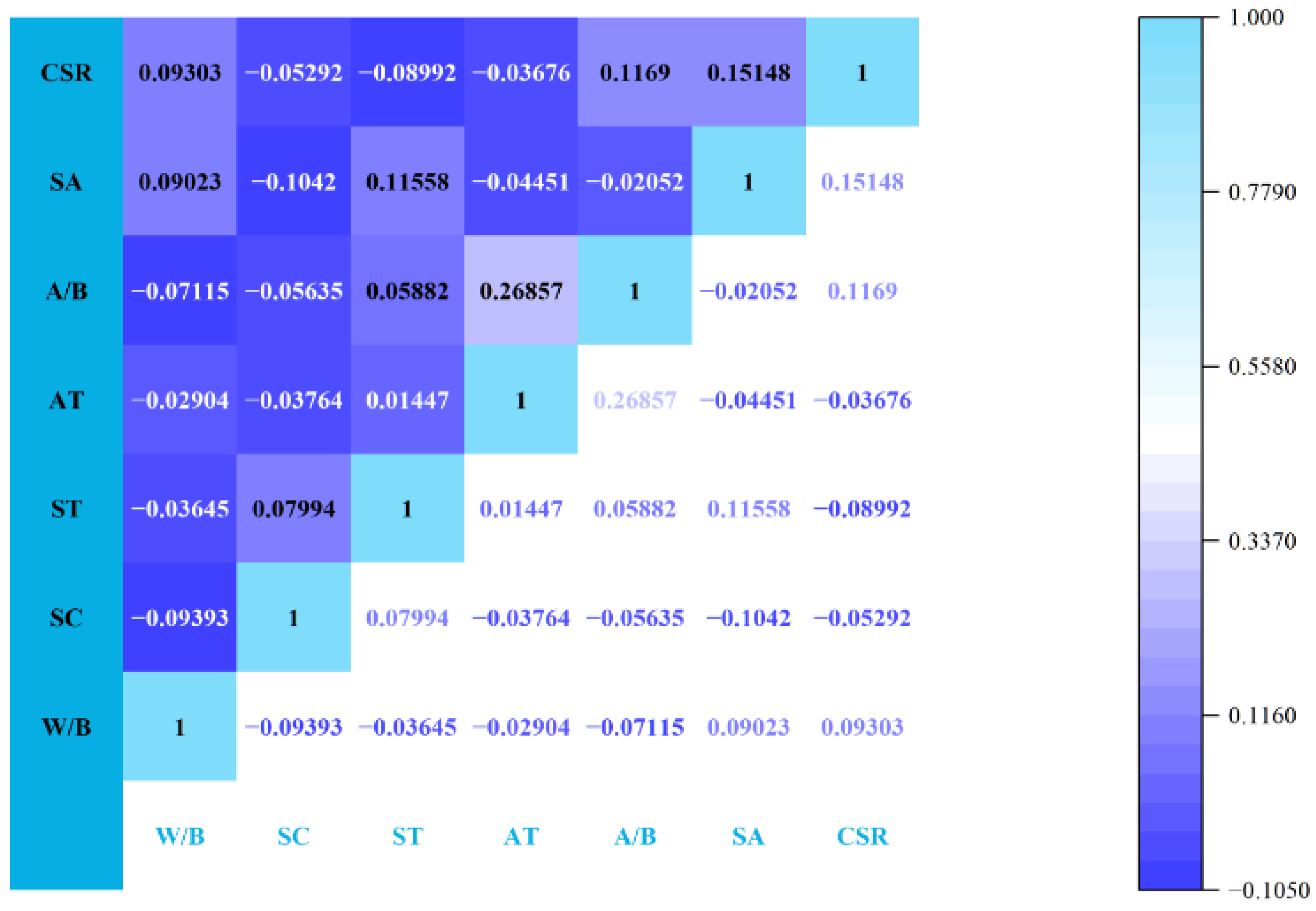
Among the inputs selected by the model, there may be variables that are redundant to each other. Therefore, Pearson correlation coefficients between input and output parameters were obtained and are displayed in
Figure 1. The technique is a measure of the strength of the linear relationship between two parameters. The correlation coefficient cannot precisely and appropriately represent the relationship strength between those two parameters if the relationship between the parameters is not linear. Statistically, the range is [−1, 1], where ‘1’ represents a flawless positive linear relationship between variables, ‘−1’ pinpoints a perfect negative, and ‘0’ indicates no linear relationship. The efficiency of the model will become low when the correlation coefficient between the input variables is a negative of a high positive. This is because they are not independent of each other. Fortunately, the situation mentioned above does not appear in this model. It is shown that the correlation between CSR and the input parameter of the SA is still positive.
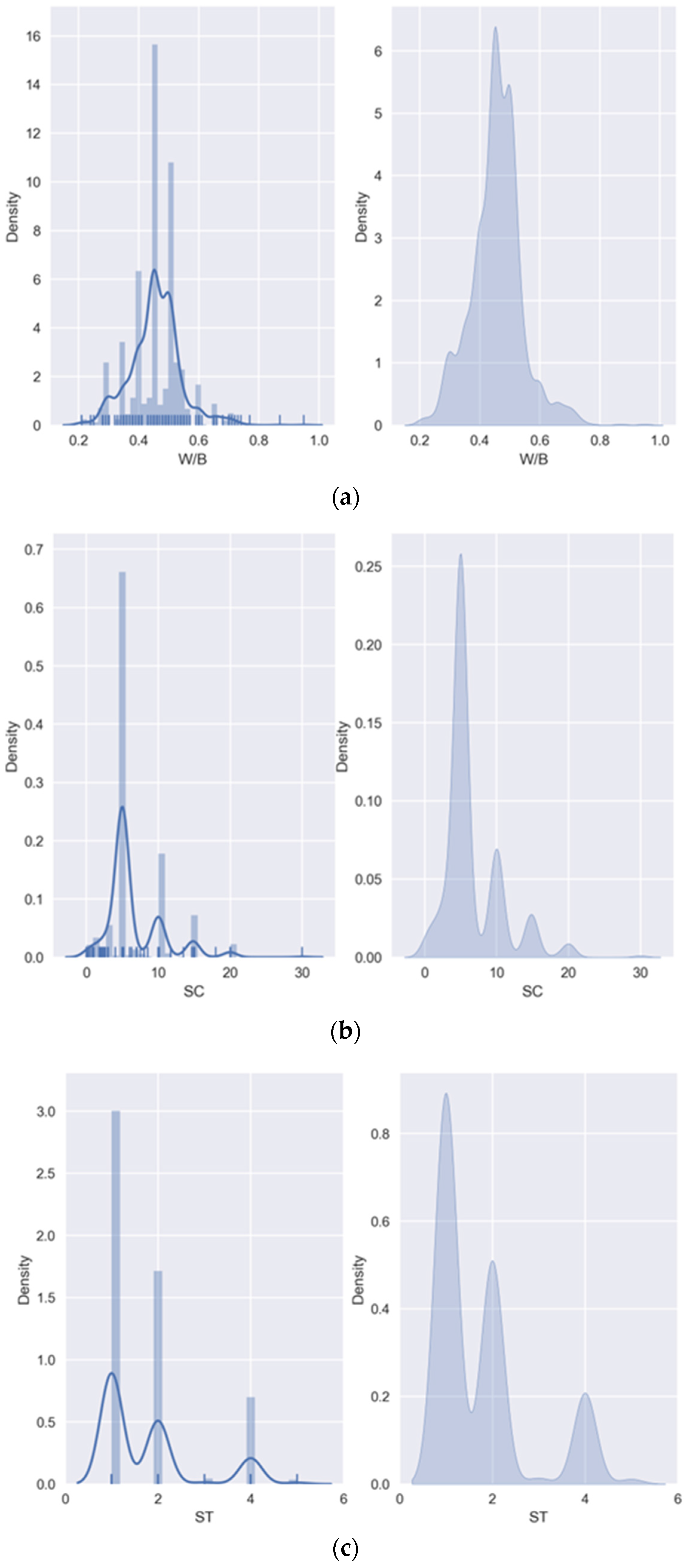
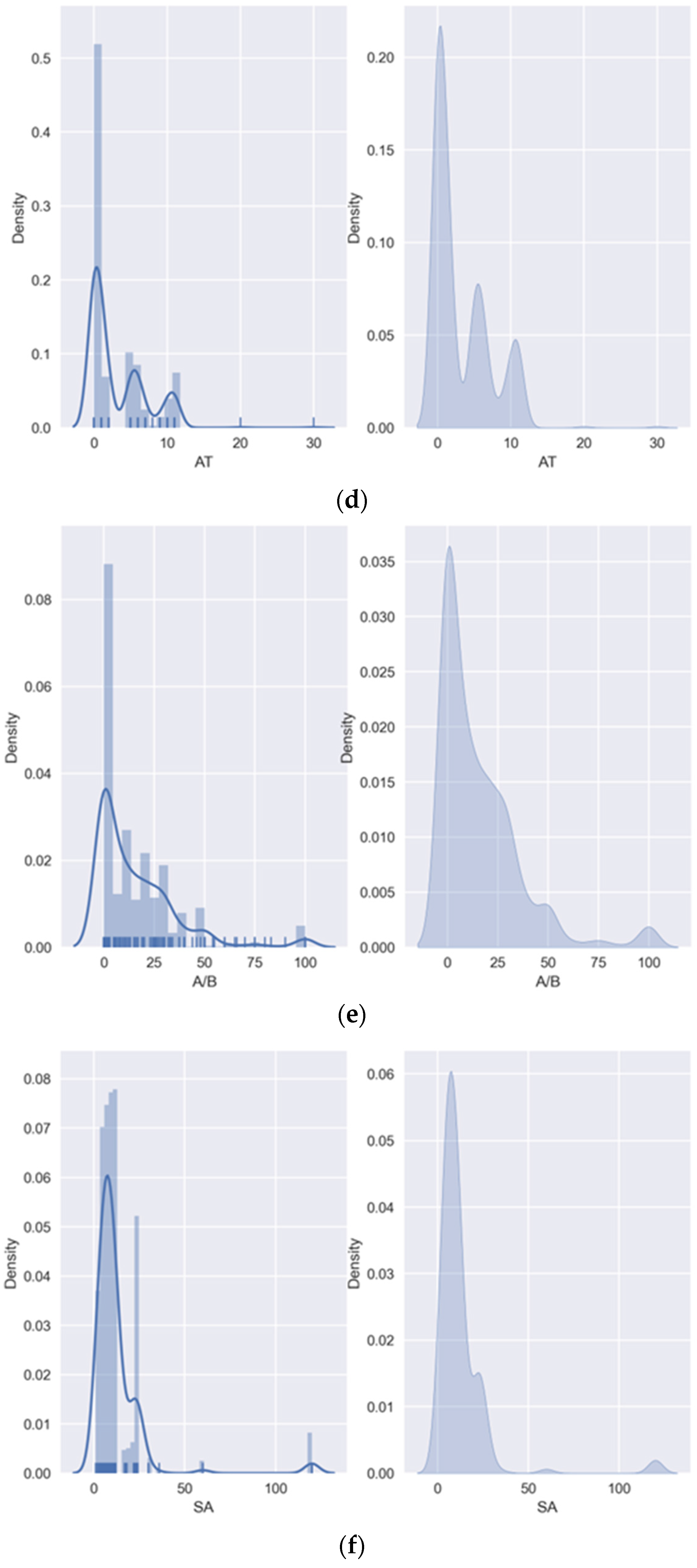
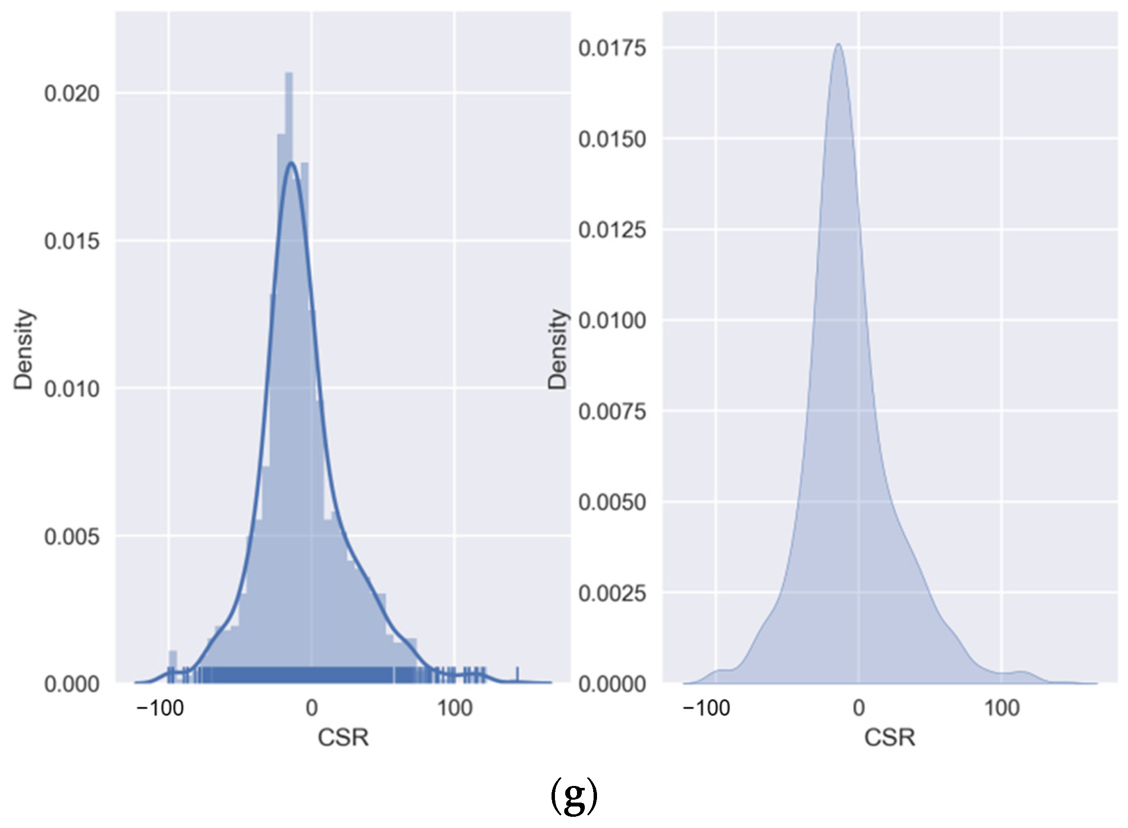
In addition, the distribution of the variable values should be noted. Solving the distribution density function of random variables with a given sample set is one of the basic problems of probability statistics. The solutions include parametric estimation and nonparametric estimation. Parameter estimation requires basic assumptions, and there is often a large gap between it and the actual physical model. Therefore, the nonparametric estimation method is a good alternative; kernel density estimation (KDE) is one of the better methods. It does not use the prior knowledge of data distribution and does not attach any assumptions. It is a method used to study the characteristics of data distribution from the data sample itself and calculates the distance of data points by weighting, and the results are shown in
Figure 2. The theory of weighting the distances of observations (
) from a particular point
is as follows:
where
is the chosen Kernel (weight function) and
is bandwidth. These figures are exceedingly advantageous, because through them, researchers can understand the distribution scope of the data and whether the amount of data is sufficient. It can be seen from
Figure 2 that the amount of data used in this study is sufficient and the distribution is reasonable.
3. Results and Discussions
The goal of the calculation investigation is to evaluate the CSR by applying 1328 sets of data. To this aim, 70% of all the data (i.e., training dataset of 930 samples) were employed to train the models, while the remaining data (398 samples) were utilized for testing. This indicated that the training effect of the model was satisfactory if the error of the training set was similar to that of the testing set. On the contrary, it indicated that there was an overfitting problem in the model if the error of the testing set was much greater than that of the training set. To evaluate the strength of fit and the robustness of the DL model, five performance parameters (loss functions) are used to assess the predicting achievement. Then, this section explores the performance of the model. Finally, a thorough comparison between the performance of existing analytical ML models and the proposed DL model is investigated.
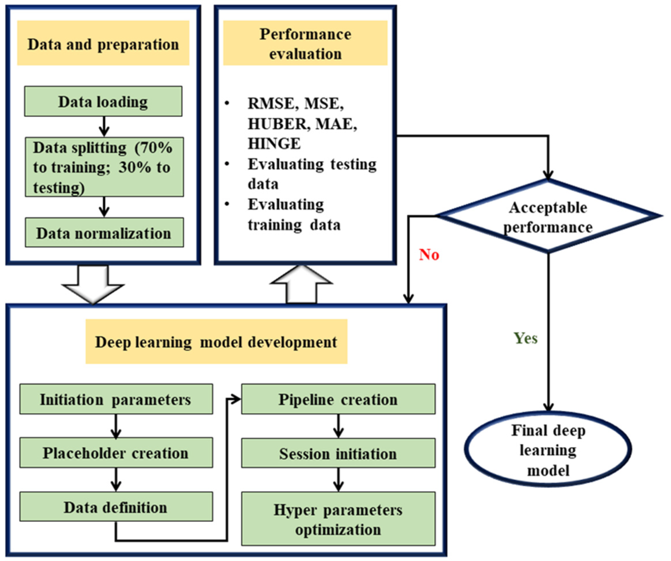
Figure 3 presents, in detail, the flow chart of the DL model based on the TF framework used in this paper. In what follows, the model performance indicators, development, and results are shown and discussed comprehensively.
3.1. Model Performance Indicators
Metric is applied to assess the performance of the model. It mainly includes the root mean square error (RMSE), mean absolute error (MAE), mean square error (MSE), HUBER, and HINGE. The following are the principle, the scope of application, and the limitations of each loss function.
The MAE measures the average error amplitude, the distance between the predicted value , and the real value , and the action range is 0 to positive infinity. It is more robust to outliers on the line. However, the derivative at point 0 is discontinuous, which makes the solution efficiency lower and the convergence speed slower. For smaller loss values, the gradient is as large as that of other interval loss values.
The MSE measures the square sum of the distance between the predicted value and the real value, and the scope of action is consistent with the MAE. There is something about the fast convergence speed. It can give an appropriate penalty weight to the gradient instead of the same, so that the direction of the gradient update can be more accurate. The disadvantage is that it is very sensitive to outliers, and the direction of the gradient update is easily dominated by outliers, so it is not robust.
The HUBER function combines the MAE and MSE and takes their advantages. The principle is to use the MSE when the error is close to 0 and to use the MAE when the error is large.
The HINGE function cannot be optimized using the gradient descent method, but needs a sub-gradient descent method. It is a proxy function based on a 0–1 loss function.
The RMSE is the square root of the ratio of the square sum of the deviation between the observed value and the real value to the number of observations, which is more sensitive to outliers.
is defined as using the mean as the error benchmark to evaluate whether the prediction error is greater than or less than the mean benchmark error. Generally, it is more effective in a linear model. It cannot fully reflect the prediction ability of the model, and cannot represent the good generalization performance of the model. The specific equations are as follows:
where
is a constant,
represents the observed value, and
is the average output of the data.
3.2. Model Developments
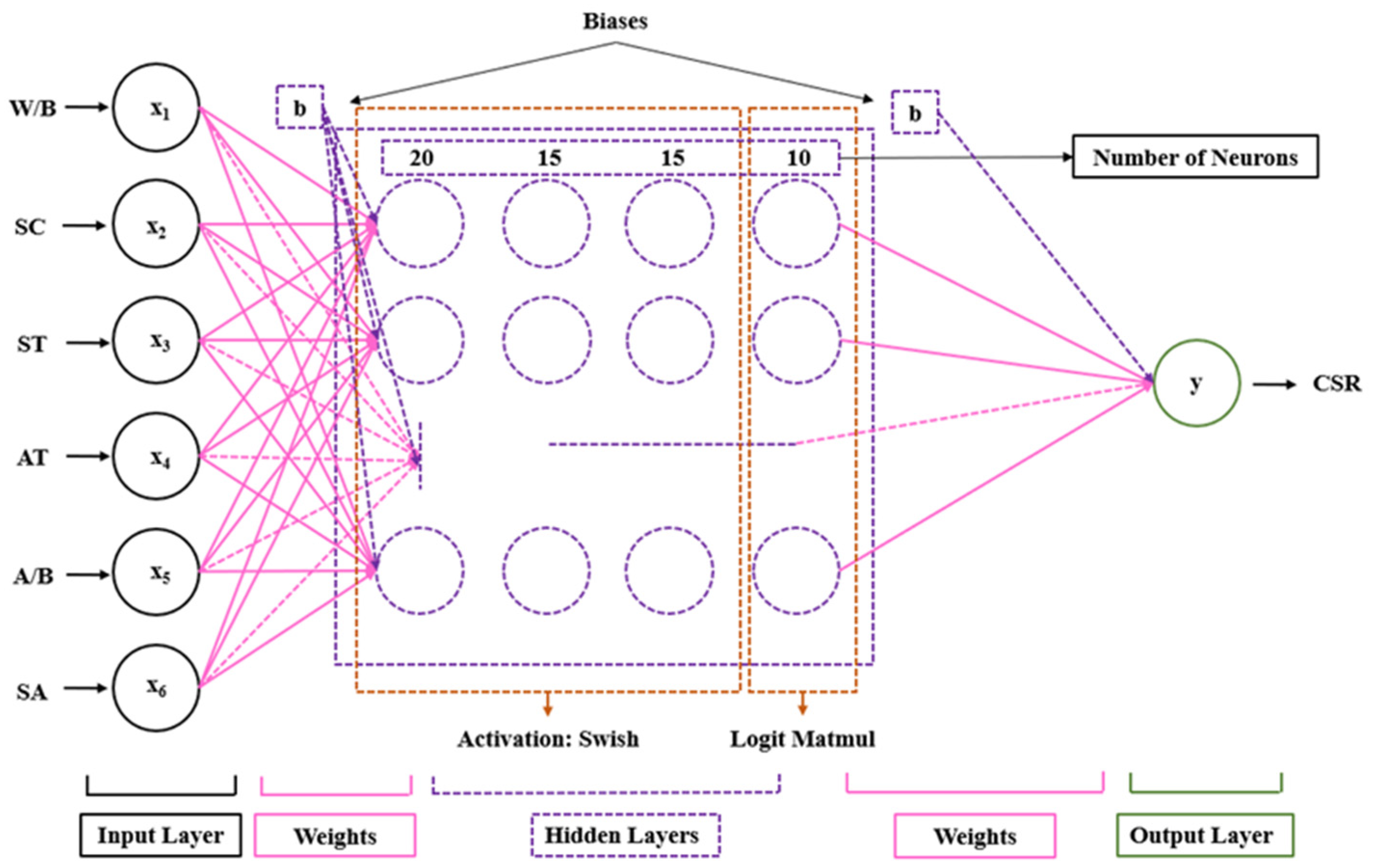
The performance of the DL model largely depends on the number of layers, the neurons in each layer, the activation function, and the hyper parameters. The optimal selection of these parameters was obtained through countless experiments. In this process, the control variable method was used for the initial parameters, and one of the parameters was modified when the other parameters remained unchanged. Because DL is usually applicable to big data, the amount of data in this study was not enough to support the excessive number of hidden layers. Therefore, it was finally determined that four hidden layers were the most appropriate number combined with the tests. The number of hidden layers and neurons in each layer can be obtained simultaneously through tests. On this basis, different activation function effects were tested. The same method was used to determine the hyper parameters. The batch size is usually set as a multiple of two, and this model was tried according to this law. The learning rate base was combined with its decay rate, and was tested from 0.001, and gradually enlarged. The regularization rate and exponential moving average decay rate are usually set 0.001 and 0.99, respectively. And the model had excellent results after the tests, so they were not modified. The number of training steps depended on the specific loss function attenuation and the use of a GPU.
Figure 4 and
Table 2 presents the activation functions and neuron number of every layer of the DL model.
Table 3 shows the optimal hyper parameters of the DL model in this study.
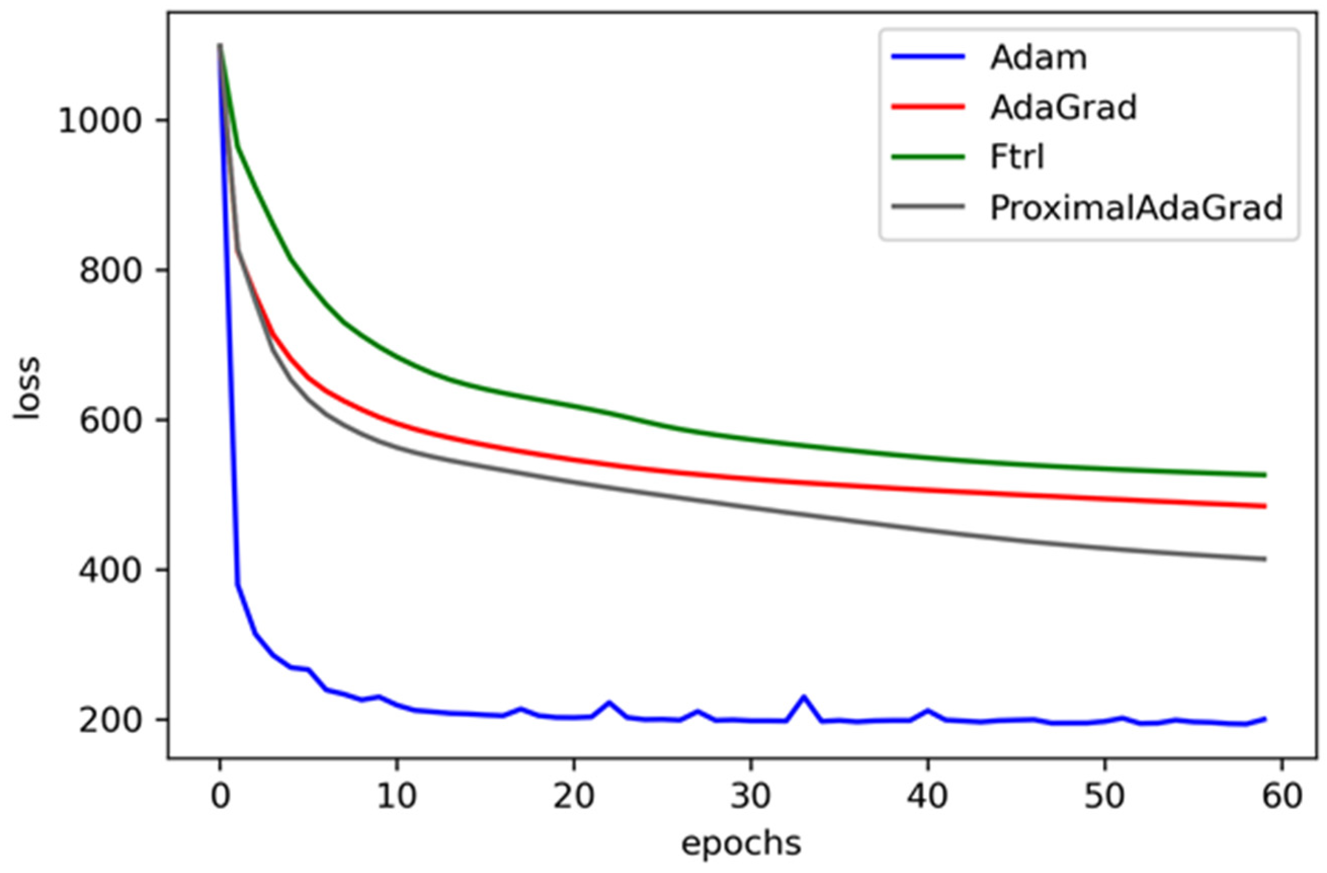
The choice of the optimizer was determined by the decline in the loss value.
Figure 5 contrasts the performance of various optimizers, including Adam, AdaGrad, Ftrl, and ProximalAdaGtrad. It can be seen that the Adam method performs best in the loss descent curve, both in speed and convergence accuracy. This is because it is computationally efficient, requires less memory, and the update of parameters is not affected by the scaling transformation of the gradient. And the hyper parameters are well interpretable, and usually do not need to be adjusted or only require a little fine-tuning, which is very important for engineering applications. For the problem of CSR prediction, it is suitable for a sparse gradient and a large noise, so the effect is so significant.
3.3. Evaluation of Model Performance
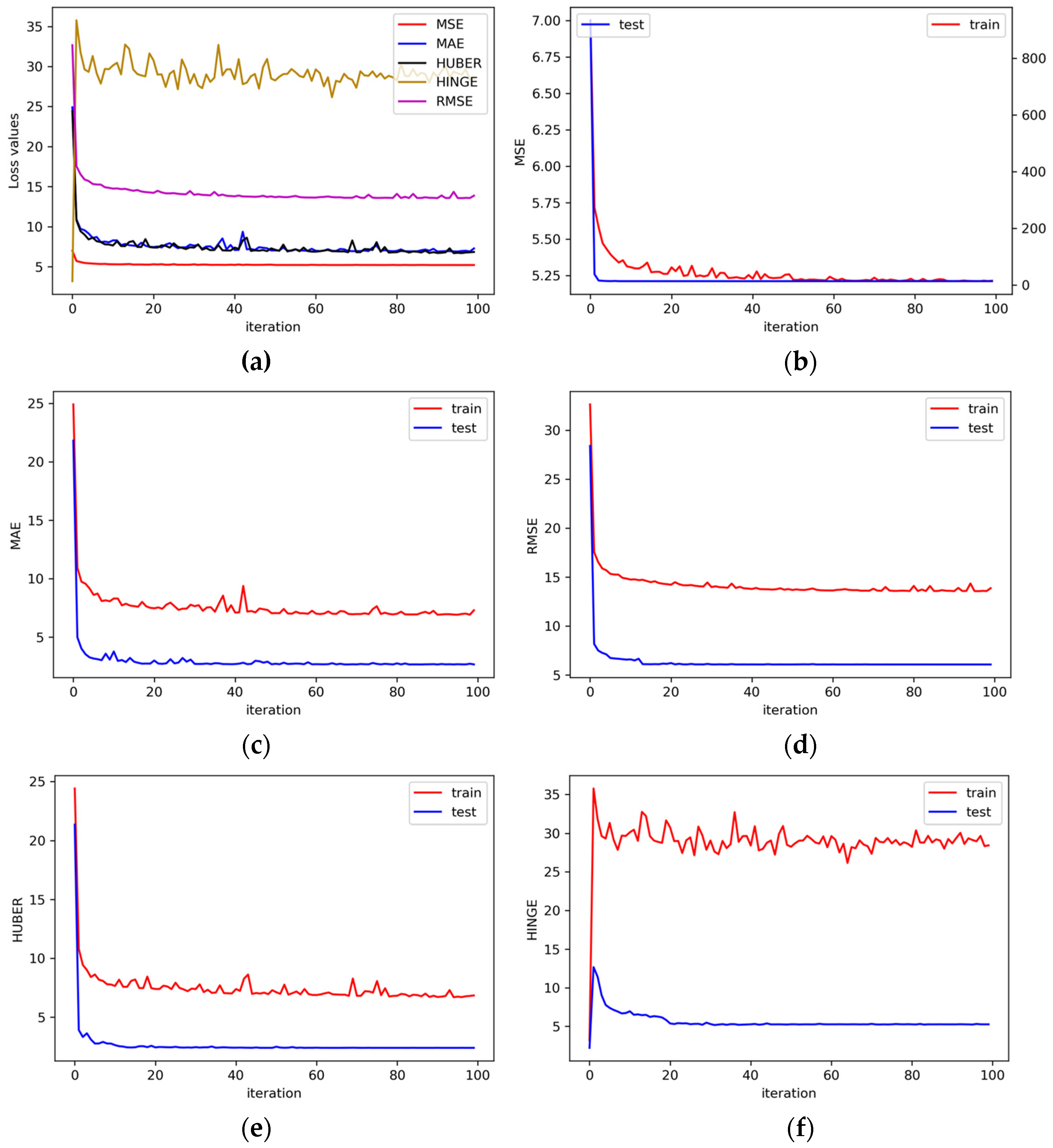
The performance of the DL model was assessed based on the MSE, MAE, HUBER, HINGE, and RMSE while considering the testing phase and training phase. Evaluating the performance of the DL model from various perspectives is the reason for choosing these indexes. For comprehensive discussion, the evaluation results of the DL model are shown in
Figure 6. Among these figures,
Figure 6a shows the performance of five loss functions on the training phase. It can be seen that MSE can converge to the minimum value the fastest; the minimum results of the MAE and HUBER are similar, but the decline process fluctuates and is unstable; the result of the RMSE is relatively stable, while the value of HINGE is the largest and the most unstable. These functions jointly show the performance of the model. The result of the minimum value and whether it fluctuates in the decline process are affected by its calculation process. It is inappropriate to specify a loss function alone, which depends on the trend of several combinations. Among them, the value of the HINGE function (
Figure 6f) rises first and then fluctuates, and there is no obvious downward trend. The reason for this abnormal phenomenon is that it is more suitable for the classification prediction model, and it fails in this regression model. Among the other loss graphs, only the testing phase of the MSE (
Figure 6b) has different coordinate axes. This is because the MSE is more sensitive to outliers. Therefore, the loss value is large in the process of initial learning iteration, but the error of the final training phase gradually tends to 0, and the decline speed is very fast. It is necessary to compare the results of the testing and training phases because the overfitting problem may still occur even if the regularization method is used. On the whole, the prediction results of the training and testing phases are very good, and it proves that the model has not over-fitted because the loss value of the training phase does not far exceed that of the testing phase. On the contrary, in
Figure 6c–e, the loss value of the training phase is even greater than that of the test set, which is not a problem with the model, but shows that the amount of data in the training phase is large, including some abnormal points, resulting in the error being greater that of the testing phase. This is a normal phenomenon in data science prediction.
3.4. Visual Interpretation of Results
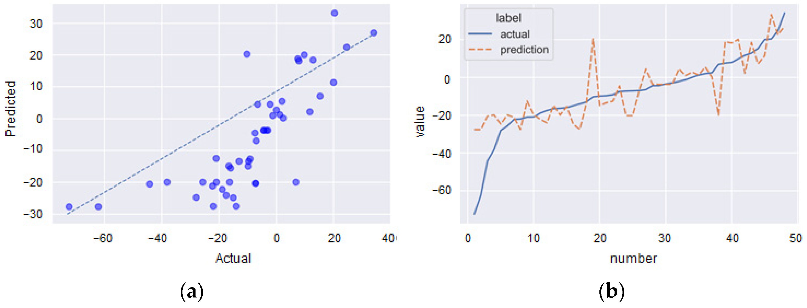
Table 4 presents the validation set that consists of 48 groups of randomly selected data from the total dataset. Intuitively, it can be seen from the table that most CSR values are negative, and the prediction in the negative range is relatively closer to the actual value. Individual results have large deviations, such as Numbers 19 and 38; the error comes from the fact that the value of W/B is too small for the Number 38, and the correlation between W/B and CSR is large. Most of the values of W/B in the data are concentrated between 0.4 and 0.6; the error of Number 38 comes from the fact that the other input values are similar, but the CSR is negative. Such a large error result is also the reason why the loss value does not fall to zero and it is a normal situation. It is impossible for any model to obtain accurate results for each set of data.
Figure 7 shows the relationship (dispersion (a) and value (b)) between the predicted and actual values through the validation set. The intuitive comparison cannot illustrate all aspects of the results, and the error band is introduced to explain the results. It can be seen from the DL model that the CSR produces a pretty close estimation with low dispersion and small measurement errors.
3.5. Comparison with Other Machine Learning Methods
3.5.1. Regression
In regression analysis, if there are two or more independent variables, it becomes multiple linear regressions (MLPR). The purpose of MLPR is to construct a regression equation and estimate the dependent variable by using multiple independent variables so as to explain and predict the value of the dependent variable. In addition to the most basic MLPR, there are various kinds of regression algorithms. This paper also used classical k-nearest neighbor regression (KNNR). The advantage of the KNNR model is that it can obtain a relatively accurate performance without too many variables, and the speed of constructing the model is usually very fast. However, the effect will become worse for datasets with more 0 values. Therefore, although the KNNR algorithm is easy to understand, it is not suitable for this study because of its slow prediction speed and because it cannot deal with multi-feature datasets.
3.5.2. Ensemble Learning
ML is chiefly divided into supervised learning and unsupervised learning. The learning model is stable in all aspects. Ensemble learning combines multiple weak supervised learning models to obtain a better and more comprehensive strong supervised learning model. Among them, the random forest (RF) algorithm establishes a forest in a random way. The forest is composed of many decision trees (DT), and there is no correlation between each DT. Each DT predicts the input, and the average result is the output of the RF. Each DT belongs to a weak learner and may become strong when combined. Bootstrap aggregation (Bagging) combines logistic regression and DT for calculation. In fact, the RF algorithm is an evolutionary algorithm of bagging. The improvement is mainly aimed at the establishment of DT. DT in bagging selects an optimal feature of all the data features on the node to divide the right and left sub-trees of the DT. However, RF randomly selects some sample features on the nodes so as to improve the generalization ability. The calculation process of the extremely randomized trees (ET) algorithm is very similar to RF, with only one significant difference. RF obtains the best splitting attribute in a random subset, while ET is completely random, so ET has better consequences than the RF algorithm in some problems.
In addition to bagging methods, boosting is also an important strategy in ensemble learning. Contrary to the parallel idea of the bagging method, boosting trains a weak learner with an initial weight from the training set, and then updates the weight of the sample according to its error rate. This process makes the weight of samples with a high error rate higher, so it is more valued in the second learner. The second learner is trained based on the adjusted weight. This belongs to tandem thought. Extreme gradient boosting (XGBT), adaptive boosting (AB), and gradient boosting (GB) are the most widely used in the boosting method. GB also combines DT models. Note that GB uses the gradient boosting method for training, while gradient descent is often used as a training method in logistic regression and ANN. The comparison of the two methods is shown in
Table 5. It can be noted that the information of the loss function relative to the negative gradient direction of the model can be used to update the current model in each round of iteration. Nevertheless, the model is expressed in parametric form in the gradient descent. Hence, the update of the model is equivalent to the update of the parameters. In gradient boosting, the model does not need parametric representation, but is directly defined in the function space, which greatly expands the types of models that can be used. The idea of the XGBT algorithm is the same as that of GB, but some optimizations are made. The second derivative is used to make the loss function more accurate, and the regular term avoids tree overfitting. The AB algorithm is different from the other two algorithms. AB emphasizes adapting. It continuously modifies the sample weight and adds weak classifiers to the boost. The other two are designed to continuously reduce the residual and establish a new model in the direction of a negative gradient by adding new trees.
3.5.3. Score Analysis
All of the above-mentioned algorithms are essential basic algorithms in supervised learning, and are calculated based on the essence of regression prediction. Therefore,
evaluation is enough to compare its applicability and accuracy in this problem.
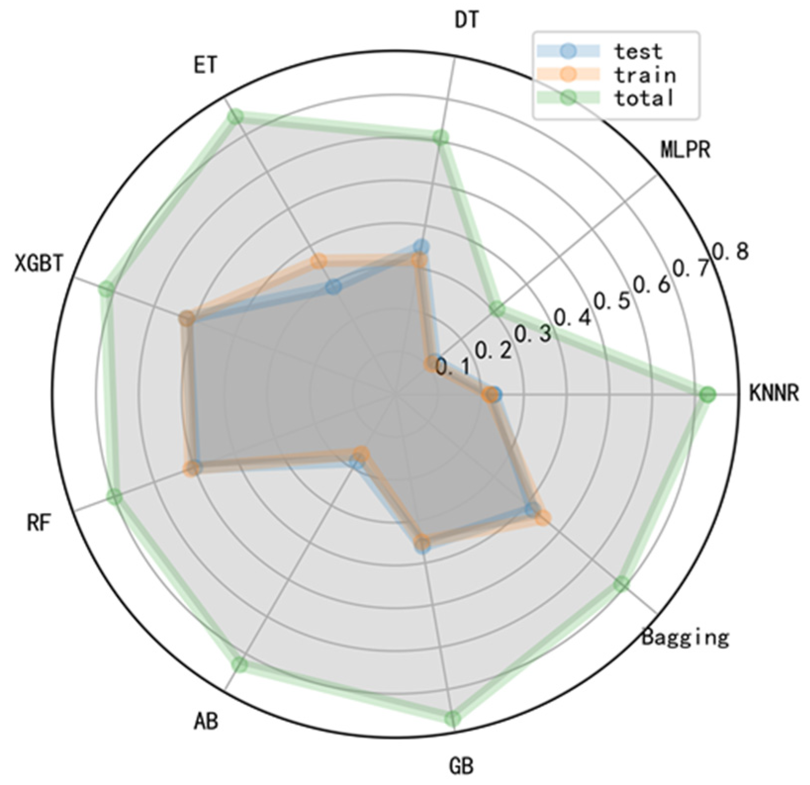
Table 6 and
Figure 8 present the results of the
analysis, from which it can be seen that in terms of the total data, except for the MLPR model, the values were between 0.60 and 0.80. The amount of total data was large, so the prediction result was relatively good. In terms of the training phase and testing phase, only the results of XGBT and RF were greater than or equal to 0.50. The results of the two regression algorithms were not very good, which were not applicable to this problem. From the side, it also reflected that the traditional regression method was not suitable for complex prediction problems. Among ensemble learning, the effect of the basic DT model was the worst, and the effect of bagging was also general. Only RF and XGBT had better effects and were relatively stable. The predicted values for the training phase and testing phase were similar, which indicated that the DL method had a certain generalization capability. However, the overall effect of the above models was not as good as the DL model, even if the DL model did not use the
evaluation method.
Because
depends on the variance of output variables, it is a measure of correlation, not accuracy. For these basic regression and ensemble learning algorithms in machine learning,
can be used to compare, but it is not suitable for complex networks such as the DL model. Moreover, the problem predicted in this paper was more complex. There is not a direct formula to calculate the change of concrete compressive strength caused by sulfate corrosion, and the internal reaction mechanism is not completely clear. And the direct and indirect relationship between the generated products and compressive strength is only qualitative, but its interaction is not clear. In addition, the amount of data (1328) is relatively large compared with the general concrete performance prediction problems, i.e., 144 and 120 samples for flexural and compressive strength [
30], 254 samples for failure modes [
35], 241 samples for ultimate compressive strength [
36], 214 samples for shear capacity [
37], and 209 samples for compressive strength [
38]. The quality of the data is naturally uneven, and the data with large separation are not eliminated. Because the actual project may also have such large dispersion data, they cannot be deleted due to the reduction in prediction accuracy. On the contrary, when the data quality is not high, it can also predict the change in the relative compressive strength, which is more favorable for practical engineering. In general, the prediction results of the DL model can be adopted by engineering practice. Predicting the compressive strength in advance in the whole life cycle of a concrete structure will be of great benefit to structural design, urban and water management, and sustainability.
4. Conclusions
It is pertinent to mention that a reliable and accurate evaluation of the CSR can provide ways to evaluate concrete buildings’ absorption of sulfide pollutants in water and can further make urban sustainability and building capacity predictable. The essential purpose of this method was to apply a soft computing method to evaluate the CSR under a sulfate attack. The model adopted optimization algorithms including mini-batch size, exponential moving average decay, and exponential decay of learning rate. It was proven that the proposed DL model can well predict the CSR of concrete caused by sulfate corrosion by analyzing the decline process of five loss functions in the testing phase and the training phase and the error comparison results between the real and the predicted value. It eliminated the need for expensive tests and saved the time cost. In addition, several traditional machine learning models, two regression algorithms, and seven ensemble learning algorithms were not suitable for this problem. The prediction accuracy of these traditional machine learning models in the training phase was not high, and the results of the testing phase were even worse, indicating that the generalization ability of these models was not good as the DL model.
In summary, the DL model is suitable for predicting the degradation performance of building materials after absorbing pollutants. Although this paper only predicts the performance after sulfate ion corrosion, the deep learning model can be extrapolated to other water pollutants when there are sufficient data.
