Article

Water Distribution Network Optimization Model with Reliability Considerations in Water Flow (Debit)

by
Herman Mawengkang
1,*,
Muhammad Romi Syahputra
1,
Sutarman Sutarman
1 and
Gerhard Wilhelm Weber
2,3
1
Department of Mathematics, Universitas Sumatera Utara, Medan 20155, Indonesia
2
Faculty of Engineering Management, Poznan University of Technology, 60-965 Poznan, Poland
3
Institute of Applied Mathematics, Middle East Technical University, Ankara 06800, Turkey
*
Author to whom correspondence should be addressed.
Water 2023, 15(17), 3119; https://doi.org/10.3390/w15173119
Submission received: 4 August 2023 / Revised: 24 August 2023 / Accepted: 29 August 2023 / Published: 30 August 2023

Abstract

:
Water distribution networks (WDNs) are defined as the planning for the development, distribution, and utilization of water resources. The main challenge of WDNs is to preserve limited water resources while providing effective benefits from these resources in accordance with environmental considerations. Water distribution networks use hydraulic components to connect water resources to consumers. The diameter of each pipe, the layout of the pipe network, and the total length of pipes all contribute to the most effective layout for a water distribution system. This study considers the assurance that the flow (discharge) of water is in accordance with what is expected, with such aspects apt to be described as a particular form of reliability. As a result, this study proposes a stochastic optimization model with non-linear probability constraints for overcoming the challenges of water distribution networks while taking water flow reliability into account. The pressure drop equation causes the non-linear shape. The stochastic model of the opportunity constraint is changed to a deterministic multi-objective model using an approach based on integer programming and sample averaging to solve the resulting model. The direct search approach (neighbourhood search) is then applied to tackle the integer part.

1. Introduction

A water distribution network (WDN) is a complex system consisting of pipes, pumps, valves, and storage facilities used to distribute potable water from a water treatment plant to consumers in a particular area. The main goal of a WDN is to distribute drinkable water to every consumer who needs it in sufficient quantity and at proper pressure. Though some cities have distinct distribution systems, for example a high-pressure system for firefighting or a wastewater recycling system, natural resources in urban areas must also be able to provide potable drinking water as well as non-potable water for use in firefighting, irrigation, etc.
This WDN consists of a network system of pipes or links (by which the water flows), which are connected at nodes (junctions) which may be at different heights. In general, a water distribution network also includes pumps, reservoirs and valves. A node in the network usually has one of two important functions, namely receiving the water supply for the system or delivering the water needed by consumers. WDN problems with multi-period patterns are grouped into mathematical optimization modelling which contains thousands of constraints and variables that are bound to one another so that a significant representation of the system is obtained.
Previous research on natural resources has tended to relate to the design of the collective pressure of the WDN so that it is able to meet consumer demand [1]; to the optimal network layout design so as to minimize the total network cost [2]; to the resolution of hydrant discharge according to the size of the location of the water distribution [1]; to the determination of the design of water flow per pipe, in accordance with a predetermined supply guarantee [3]; to the calculation of optimal pipe diameter size to minimize investment and energy costs [4]; and to the analysis of network enactment under various operating conditions [5] in order to find out in which situations a failure of the water supply from the network or water pump source is likely to occur [6]. Lubis and Mawengkang [7] have also presented a model that contains reliability in water flow.
Other WDN studies that have been developed, such as the study described in [8], have assessed the reliability of the water distribution system without evaluating all possible mechanical pipe failures. Liu et al. [9] devised a prediction approach that distinguishes the pipe parts that are likely to be impacted the most without investigating the hydraulic performance of the pipe for each probable failure circumstance. Kalungi and Tanyimboh [10] addressed the question of how to reliably evaluate system performance via the use of redundancy and backup. The critical head-driven simulation approach is used to conduct system dependability research. However, the focus of this research is solely on the dependability of network topology. In an effort to enhance distribution service and dependability, Jun et al. [11] devised a mechanism that calculates how much of an effect a broken pipe or a moved valve would have on the overall water supply system. This was undertaken to enhance the distribution service. Nazif and Karamouz [12] used the system readiness index to assess the resilience of a WDN for one or more primary reservoirs of water. A system’s dependability, robustness, and vulnerability were all assessed during this evaluation. The previous study is still linked to the evolution of the variability of the techniques and methodologies that were created in the past. However, in reality, natural resources contain uncertain parameters, especially in dealing with the reliability of water discharge and water quality.
There is no discussion of a WDN model that handles the reliability of water discharge and water quality with uncertain parameters in the literature. Mathematically, the problem of distributing water pressure in a water distribution network, developed from the Hazen–Williams equation, can be formulated as a problem of finding the roots of a system of non-linear equations which are generally large in size. The non-linear form that results does so due to the water pressure drop equation, which is itself a stochastic model equation [13]. Completion of the stochastic model with the integer programming model continues to create difficulties because it is related to the solving of the optimal feasible basic vector components of a system that is continuous and sustainable. Meanwhile, the distribution network system must take client demands into account by prioritizing the dependability of water distribution services. For this reason, a network system model is needed that can overcome the reliability of water distribution services.
This theoretical overview looks at the many approaches to modelling and designing water distribution networks, focusing on its inherent vulnerabilities. Each vulnerability discussion will centre on one of the seven components of the water distribution system defined by [14]. System vulnerability can also be measured using dependability, robustness, and redundancy; however, these three factors will be discussed and measured in different ways.
Aklog and Hosoi [15] proposed an innovative model known as the all-in-one approach for designing water distribution network (WDN) systems. This approach integrates linear programming and genetic algorithms to create optimized network designs. Meanwhile, Tanyimboh [16] conducted an in-depth analysis using the cut set and reachability procedure, offering insights into resource reliability. However, this traditional methods impracticality for urban networks became evident as it could not account for all of the potential mechanical pipe failures.
To address this limitation, Tanyimboh [16] adapted their analysis by considering the most likely simultaneous failures of specific pipes based on real-world data. Simulation of failure scenarios provided a probability assessment, taking into account the quantity of pipes potentially going out of service. Conversely, assuming uniform failure likelihood for all pipelines allowed for streamlined analysis, albeit without accounting for natural disasters or human-induced devastation.
Bagloee et al. [17] devised a hybrid strategy merging regression models and optimization techniques to enhance resource efficiency. Similarly, Liu et al. [9] introduced a prediction method that identifies high-risk pipe segments without necessitating a comprehensive hydraulic analysis for each failure scenario. In cases where a comprehensive understanding of water flow from transmission components is crucial, microflow distribution has proven to be effective. This approach considers debit rates and node ingress and outgress, ensuring uniform circulation across connected conduits.
Emphasizing the importance of redundancy and dependability, Kalungi and Tanyimboh [10] employed a head-driven simulation approach to assess system efficiency. This analysis surpassed traditional demand-based assessments by incorporating pressure considerations at nodes. Lippai and Wright [18] evaluated network performance under normal and failure conditions, determining pipe importance by assessing pressure differences. The need for a separate hydraulic study for each potential failure scenario posed limitations in practical urban networks.
To optimize system robustness, Qiao et al. [19] presented a quantitative approach focused on minimizing economic impacts during network assaults. This methodology integrated genetic algorithms and simulation, creating an effective tool for resource protection. Jun et al. [11] developed an algorithm to quantify the effects of damaged pipes or valves on the overall network, emphasizing the need to consider multiple simultaneous failures.
Wang and Au [20] prioritized critical pipelines post-earthquake through a novel strategy involving the damage consequence index (DCI) and upgrade benefit index (UBI). This approach considered spatial variability in system reliability and resource distribution. Meanwhile, Nazif and Karamouz [12] introduced the system readiness index (SRI) for assessing preparedness against pipeline breaks. This index factored in dependability, resilience, and vulnerability, providing insights into network performance.
Further enhancing assessment methodologies, Baoyu et al. [21] employed a vulnerability assessment model for regional water distribution systems (VAM-RWDS). This stochastic approach generated vulnerability indices based on various hydraulic and water quality parameters, offering a comprehensive understanding of system susceptibility.
As the quest for optimal designs continues, various optimization strategies have emerged. Linear programming gradient (LPG) [22], genetic algorithms [23,24,25], and Tabu search [25] have shown promise in solving intricate WDN problems. These approaches decompose complex challenges into manageable sub-problems or employ metaheuristic algorithms to achieve near-optimal solutions. However, converting computed values into practical pipe dimensions remains a challenge [26].
Uncertainty remains a significant challenge in WDN design and operation [27,28]. Neufville et al. [29] highlighted three strategies for managing uncertainty: uncertainty control, passive protection, and active protection. Forecasting models aim to minimize estimate errors, while passive protection methods create robust designs. However, complexities in the relationship between uncertainty and WDN variables hinder complete mitigation.
In conclusion, advancements in WDN analysis and optimization continue to drive innovation in network design and operation, addressing challenges from reliability assessment to uncertainty management. As researchers develop increasingly sophisticated strategies, the field continues to evolve as it aims for more efficient, resilient, and dependable water distribution systems.

2. Problem Description

This research first builds a water distribution network model in the form of a deterministic optimization, i.e., one in which all of the model parameters are known. Additionally, the computation is extended to a larger time dimension, with the size and number of time stages assumed to be sufficient to adequately reflect the changing hydrological currents and water demand in the network system, provided that the time phase (period) t is assumed to be constant. By considering a static water distribution network system or in a single period situation, the concept of graph theory can be used to represent the network system derived from a physical sketch of a cluster. The nodes can represent water sources, water demand, reservoirs, groundwater, diversion canal sites, hydropower sites, etc. By taking into account the fundamental graph for each time period, we are able to create a graphical representation of dynamic issues, which we call a multi-period dynamic network. We then connect the appropriate reservoir nodes for different successive time periods with the paths that carry the accumulating water at the end of each period.

2.1. Water Distribution Network Optimization Model Components

Several components can be used in the formation of the model. The following describes some of the components that are considered representative of the system. Refs. [30,31,32] provide more in-depth descriptions of this strategy. There is a dynamic network G = ( N , A ) where N is the set of vertices and A is the set of paths. T denotes the set of time steps t .

2.1.1. Hydraulic Network Components and Sets Required in Model Development

  • Vertices (a subset of N ): ( N as a set of vertexes and the set of natural numbers may not be confused);
    Other node sets can represent groundwater, desalinization, wastewater treatment plants, etc.
  • Aqueducts (Arcs) (a subset of A ):
    The mathematical model of system planning/design that pays attention to reliability on constraints such as this requires the optimization problem to adopt probabilistic rules on the constraints so that the optimization model that is formed becomes an optimization model problem with probabilistic constraints or opportunity constraints. A water distribution network optimization model, in its planning and application design, is inseparable from one that seeks to satisfy demands in its services. Therefore, a water distribution network optimization model is proposed by adopting probabilistic rules of several constraints that can increase service satisfaction. This water distribution network optimization model is called the chance-constrained model. In its application, we attempt to display several possible performance sets of a water distribution network system as different uncertain parameters.
    The general form of the opportunity constraint model can be written as:
m i n x X f x
Subject to
Pr { G ( x , ξ ) 0 } 1 ε
with X n presenting the feasible area, f : n the objective function to be optimized, ξ the random vector whose probability distribution is supported on the set Ξ n , G : n × d m the constraint mapping and ε 0,1 the risk parameters. This formulation determines the decision vector x that minimizes the function f x but meets the opportunity constraints G x , ξ 0 with a probability of at least 1 ε .
For water network problems, there are opportunity constraints as follows:
P r p j l π j l d j P j 1 ε
P r h j l π j l α j H j 1 β
One of the most common methods for dealing with random variables in optimization issues is chance-constrained programming. Although Charnes developed the concept of chance limited programming in 1958, it has since seen little development in terms of problem-solving techniques. The chance-constrained approach may be stated in its most basic form as follows:
min x X f ( x )
Subject to
P h x , ξ 0 p .
in this case, ξ is a random vector with a probability distribution P , p [ 0 , 1 ] is a confidence interval vector, β is a risk parameter, and β 0 , 1 , x is a decision vector. In this case p can increase far beyond the limit without affecting the optimal value of other problems, until it is close enough to 1 to be able to further clarify the optimality of the objective.
There are two reasons that make this problem difficult to solve: firstly, for each x X , the value of P ( h ( x , ξ ) 0 ) is difficult to quantify because it requires multidimensional integration. As a result, we can only examine the feasible regions given by the points x X using a Monte Carlo simulation. Secondly, the feasible region of problem (4) is a non-convex form, though the set X is convex and a function h ( x , ξ ) convex for point x . Thus, it is not surprising that there is no single solution for chance-constrained programming. The choice depends on how strongly or how randomly the decision variable is connected to the model constraints. The convexity of this model depends not only on function (4) but also on the random parameter distribution ξ . Whether the distribution is discrete or continuous is also an important issue to determine the solution algorithm.
In contrast to conventional optimization problems, chance-constrained programming has two types of approximations. First, the distribution of random parameters can hardly be known with certainty and must be estimated from the available data. Second, even for a given multivariate distribution it cannot be calculated with certainty but must be approximated through simulation. The two approximations above thus motivate the chance-constrained model in terms of stability (balance) in programming.

2.1.2. Pressure Drop

As water travels through the pipes, it encounters various resistances, such as friction against the pipe walls and fittings, changes in pipe diameter, elevation differences, and other flow restrictions. These resistances collectively contribute to a loss of pressure along the pipeline, which is known as pressure drop.
The pressure drop equation, often referred to as the Darcy–Weisbach equation, provides a mathematical relationship to quantify the pressure drop in a pipe due to friction. The equation is as follows:
P = f . L D . 1 2 . ρ . V 2
where:
  • P is the pressure drop across the pipe.
  • f is the Darcy friction factor, which depends on the roughness of the pipe surface and the Reynolds number (a dimensionless quantity describing the flow regime).
  • L is the length of the pipe.
  • D is the diameter of the pipe.
  • ρ is the density of the fluid (water in this case).
  • V is the velocity of the fluid within the pipe.
It is important to note that the Darcy–Weisbach equation is just one component of the overall pressure drop within a water distribution network. Other factors, such as elevation changes, local flow restrictions, and pipe fittings, also contribute to the total pressure drop.

2.2. Deterministic Chance-Constrained Forms

max i = 1 n a i m x i
Subject to
i = 1 n a i j x i b j   ( j = 1,2 , , m ) .
Chance-Constrained Stochastic Form
Individual Chance Constraint
max i = 1 n a i m x i
Subject to
P i = n n a i j x i ξ j p j = 1,2 , , m .
In this case the notions of each individual are separately constraint (stochastic) i = n n a i j x i ξ j transformed into chance-constrained forms.

2.3. Joint Chance-Constrained Form

P i = n n a i j x i ξ j ( j = 1,2 , , m ) p
Based on a system of stochastic inequalities h j ( x , ξ ) 0 and individual chance-constrained forms, namely:
α j x p j = 1,2 , , m ,   where   α j P h j x , ξ 0 j = 1 , , m
For joint chance-constrained forms this is
α j ( x ) p   where   α j P h j x , ξ 0 j = 1 , , m .
Formally, one of the two conditions above has become a common obstacle in optimization problems. However, neither α nor α j are given to clarify the formulation but rather to define the probability of a region of solving by random parameters ξ .
Three things that make this problem relatively difficult are:
  • Chance-constrained models (individual or joint);
  • Assumptions of random vectors (whether continuous or discrete, or independent);
  • Types of stochastic inequalities (linear, convex, right-hand random constraints).
During function h j x , ξ = g j x ξ j ( j = 1 , , m ) , this condition is said to be very helpful. In other words, for stochastic inequalities g j ( x ) ξ j , the random parameter will then appear on the right of the function. By using the distribution function F η z P ( η z ) for some random variable η the individual chance-constrained formulation becomes
α j x = P g j x ξ j = F ξ j g j x j = 1 , , m .
An individual chance-constrained model with the function on the right is based on the formulation of the stochastic constraint structure. If the structure of the last function is linear then the individual chance-constrained form will also be linear. Such a process does not apply to joint chance-constrained forms. For right-sided randomness, the constraint function on joint chance-constrained forms is stated as follows,
α j x = P ( g j x ξ j ( j = 1 , , m ) = F ξ j g j x )
where g = ( g 1 , , g m ) and F ξ j are random vector distribution functions of ξ . If the random vector ξ has independent components, then computation α becomes,
α j x = F ξ 1 g 1 x F ξ m g m x
In some simple cases, the decision variables and random variables can be combined. Therefore, constraints can be formed with a deterministic model using probability density functions and linear programming or nonlinear programming. However, it is very difficult to convert the constraint function into a deterministic form that is a matter of convexity, equilibrium, and model structuring.

3. Results and Discussion

3.1. The Algorithm

We solve the model by combining the “active constraint” technique with a method that involves releasing non-basic variables from the boundaries they are now confined to. The goal of this method is to convert all non-integer basic variables to integer values as close as possible. The criterion for selecting a non-basic variable to use in the integerizing technique has also been considered.
  • Stage 1.
Step 1. Solve the continuous problem. The result is an unfeasible integer solution.
Step 2. Obtain row i *, which contains a minimum distance to the integer result.
Step 3. Undertake a pricing operation.
Step 4. Calculate the maximum movement of non-basic j ,
min j d j α i j
If none go to next i *.
Step 5. Solve B α j * = α j * for α j *,
Step 6. Complete a ratio test for the basic variable,
Step 7. Perform exchange basis,
Step 8. If there is no other row go to Stage 2, otherwise,
Back to step 2.
  • Stage 2.
Step 1. Adjust integer unfeasible superbasics,
Step 2. Perform a neighbourhood search to verify local optimality.

3.2. Example

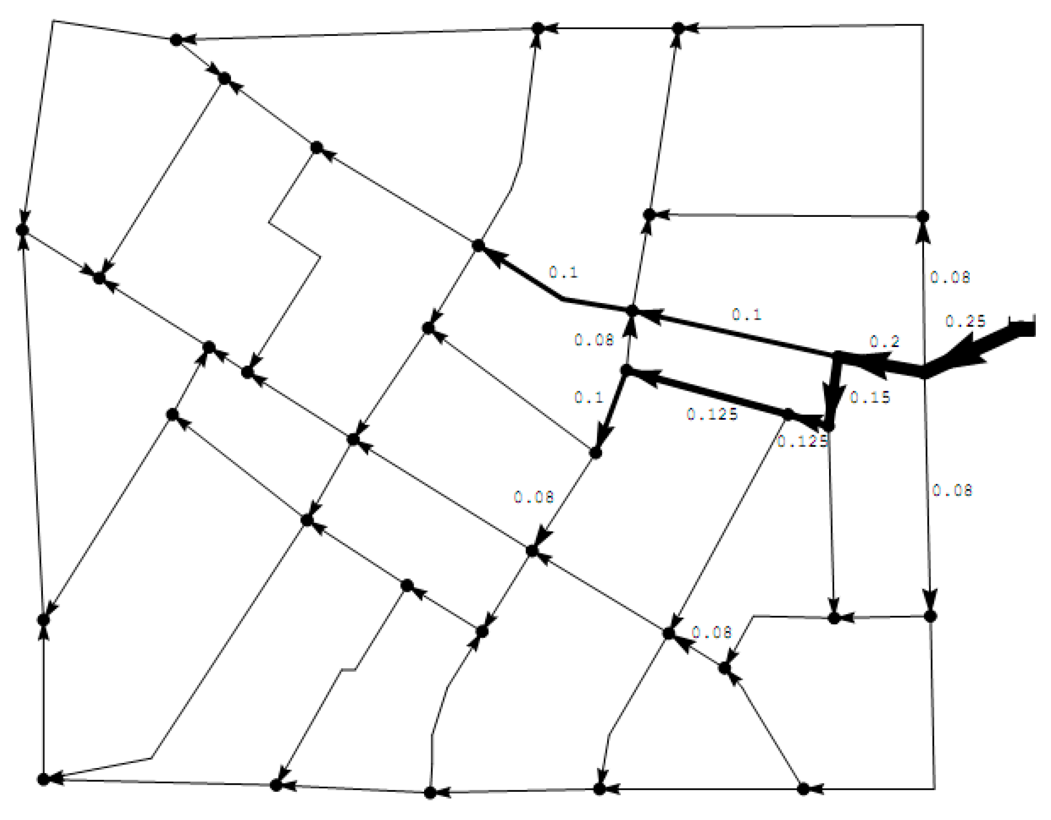
We will provide a practical illustration in the next section. There are 58 pipelines and 37 connections (the number 37 denotes the location of a single reservoir). The network topology is depicted in Figure 1, and additional information is provided in Table 1.
The hydraulic head of the reservoir remains constant under all conditions. Here, we have it permanently fixed at 121.0 m. Maximum water velocity via the pipes is restricted to 1 m3/s, and the roughness coefficient is set at 100. For all i N , the minimum allowable pressure head value, denoted by p h min ( i ) , is 40 m, while the maximum allowable value, denoted by p h max ( i ) , is 121 eval(i) meters. Table 2 describes the network’s structure and pipe lengths. In terms of the diameters of the pipes we have available, we have thirteen distinct options to choose from. Table 1 displays the ( D e , r , C e , r ) value for all r = 1 , , r e for each e E . Elevation and demand data for each junction are shown in Table 1, beside the reservoir.

3.3. Solution Found by the MINLP Model

As shown in Figure 2, the answer involves a relationship between the radius of each circle and the length of the arc drawn across it. Pipes without a diameter number are assumed to have a diameter of 0.06 m. In terms of data collecting, this is the lowest diameter feasible. This solution is analysed and found to have a set up in which the reservoir is closer to the network’s outer nodes and the diameters of the network’s components diminish as one moves away from it. This attribute of pipe diameter allocation contributes to the network’s efficient hydraulic operation and improves water quality.
It should be noted that there is no guarantee that the proposed solution is the global optimum. While the topic at hand is inherently difficult, the suggested solution is a high-quality practicable solution from a practical standpoint. Nonlinear programming models, mixed integer linear programming algorithms, and heuristic algorithms are among the alternatives; however, these also struggle with medium-to-large-scale cases. In this case, naturalistic modelling of the problem appears to be the best solution. The optimal result is shown in Figure 2.

4. Conclusions

In this paper, we have developed and presented a comprehensive water distribution network optimization model that integrates reliability considerations into the optimization of water flow. Our research aimed to address the critical need for sustainable and resilient water distribution systems, especially in the face of increasing urbanization, population growth, and potential disruptions due to natural or anthropogenic factors. Through a combination of mathematical modelling, optimization techniques, and reliability assessment, we have demonstrated the importance of considering reliability metrics alongside traditional hydraulic performance metrics. Here, we provide a paradigm for managing water resources using chance-constrained programming. We use a strategy in which constraints can be formed with a deterministic model using probability density functions and linear programming or nonlinear programming. Nevertheless, it is very difficult to convert the constraint function into a deterministic form that is a matter of convexity, equilibrium, and model structuring. A direct search technique is used to solve the resulting model.

Author Contributions

Conceptualization, H.M.; Methodology, H.M.; Writing—original draft, M.R.S. and S.S.; Writing—review & editing, G.W.W.; Funding acquisition, H.M. All authors have read and agreed to the published version of the manuscript.

Funding

This research was funded by TALENTA Research scheme, grant number 366/UN5.2.3.1/PPM/KP-TALENTA/2022.

Data Availability Statement

There is no need for data statement.

Acknowledgments

We would like to express our gratitude to the Universitas Sumatera Utara for the funding that we obtained for the TALENTA Research scheme with contract number 366/UN5.2.3.1/PPM/KP-TALENTA/2022, dated 9 August 2022.

Conflicts of Interest

The authors declare no conflict of interest.

References

  1. Huang, D.; Vairavamoorthy, K.; Tsegaye, S. Flexible design of urban water distribution networks. In World Environmental and Water Resources Congress 2010: Challenges of Change; American Society of Civil Engineers: Reston, VA, USA, 2010; pp. 4225–4236. [Google Scholar]
  2. Zhe, X.; Jie, Y.; Huaqiang, C.; Yaguang, K.; Bishi, H. Water Distribution Network Modeling Based on NARX. IFAC-Pap. 2015, 48, 72–77. [Google Scholar] [CrossRef]
  3. Liong, S.-Y.; Atiquzzaman, M. Optimal design of water distribution network using shuffled complex evolution. J. Inst. Eng. 2004, 44, 93–107. [Google Scholar]
  4. Ekinci, Ö.; Konak, H. An Optimization Strategy for Water Distribution Networks. Water Resour. Manag. 2009, 23, 169–185. [Google Scholar] [CrossRef]
  5. Coelho, B.; Andrade-Campos, A. Efficiency achievement in water supply systems—A review. Renew. Sustain. Energy Rev. 2014, 30, 59–84. [Google Scholar] [CrossRef]
  6. Izquierdo, J.; Montalvo, I.; Pérez-García, R.; Matías, A. On the Complexities of the Design of Water Distribution Networks. Math. Probl. Eng. 2012, 2012, 947961. [Google Scholar] [CrossRef]
  7. Lubis, A.; Medan, U.N.; Mawengkang, H. A Nonlinear Stochastic Optimization Model for Water distribution network problem with reliability consideration. Int. J. Comput. Trends Technol. 2014, 17, 182–189. [Google Scholar] [CrossRef]
  8. Siew, C.; Tanyimboh, T.T.; Seyoum, A.G. Penalty-Free Multi-Objective Evolutionary Approach to Optimization of Anytown Water Distribution Network. Water Resour. Manag. 2016, 30, 3671–3688. [Google Scholar] [CrossRef]
  9. Liu, H.; Savić, D.A.; Kapelan, Z.; Creaco, E.; Yuan, Y. Reliability Surrogate Measures for Water Distribution System Design: Comparative Analysis. J. Water Resour. Plan. Manag. 2017, 143, 4016072. [Google Scholar] [CrossRef]
  10. Kalungi, P.; Tanyimboh, T.T. Redundancy model for water distribution systems. Reliab. Eng. Syst. Saf. 2003, 82, 275–286. [Google Scholar] [CrossRef]
  11. Jun, H.; Loganathan, G.V.; Kim, J.H.; Park, S. Identifying Pipes and Valves of High Importance for Efficient Operation and Maintenance of Water Distribution Systems. Water Resour. Manag. 2008, 22, 719–736. [Google Scholar] [CrossRef]
  12. Nazif, S.; Karamouz, M. Algorithm for Assessment of Water Distribution System’s Readiness: Planning for Disasters. J. Water Resour. Plan. Manag. 2009, 135, 244–252. [Google Scholar] [CrossRef]
  13. D’ambrosio, C.; Lodi, A.; Wiese, S.; Bragalli, C. Mathematical programming techniques in water network optimization. Eur. J. Oper. Res. 2015, 243, 774–788. [Google Scholar] [CrossRef]
  14. Haimes, Y.Y.; Matalas, N.C.; Lambert, J.H.; Jackson, B.A.; Fellows, J.F.R. Reducing Vulnerability of Water Supply Systems to Attack. J. Infrastruct. Syst. 1998, 4, 164–177. [Google Scholar] [CrossRef]
  15. Aklog, D.; Hosoi, Y. All-in-one model for designing optimal water distribution pipe networks. Drink. Water Eng. Sci. 2017, 10, 33–38. [Google Scholar] [CrossRef]
  16. Tanyimboh, T.T. Informational Entropy: A Failure Tolerance and Reliability Surrogate for Water Distribution Networks. Water Resour. Manag. 2017, 31, 3189–3204. [Google Scholar] [CrossRef]
  17. Bagloee, S.A.; Asadi, M.; Patriksson, M. Minimization of water pumps’ electricity usage: A hybrid approach of regression models with optimization. Expert Syst. Appl. 2018, 107, 222–242. [Google Scholar] [CrossRef]
  18. Lippai, I.; Wright, L. Criticality Analysis Case Study: Zone 7 Water Distribution System. In Pipelines 2005: Optimizing Pipeline Design, Operations, and Maintenance in Today’s Economy; American Society of Civil Engineers: Reston, VA, USA, 2005; pp. 662–673. [Google Scholar]
  19. Qiao, J.; Jeong, D.; Lawley, M.; Richard, J.-P.P.; Abraham, D.M.; Yih, Y. Allocating security resources to a water supply network. IIE Trans. 2007, 39, 95–109. [Google Scholar] [CrossRef]
  20. Wang, Y.; Au, S.-K. Spatial distribution of water supply reliability and critical links of water supply to crucial water consumers under an earthquake. Reliab. Eng. Syst. Saf. 2009, 94, 534–541. [Google Scholar] [CrossRef]
  21. Baoyu, Z.; Xinhua, Z.; Yuan, Z. Vulnerability assessment of regional water distribution systems. In Proceedings of the 2009 International Conference on Environmental Science and Information Application Technology, Wuhan, China, 4–5 July 2009; pp. 473–477. [Google Scholar]
  22. Alperovits, E.; Shamir, U. Design of optimal water distribution systems. Water Resour. Res. 1977, 13, 885–900. [Google Scholar] [CrossRef]
  23. Simpson, A.R.; Dandy, G.C.; Murphy, L.J. Genetic Algorithms Compared to Other Techniques for Pipe Optimization. J. Water Resour. Plan. Manag. 1994, 120, 423–443. [Google Scholar] [CrossRef]
  24. Cunha, M.d.C.; Sousa, J. Water Distribution Network Design Optimization: Simulated Annealing Approach. J. Water Resour. Plan. Manag. 1999, 125, 215–221. [Google Scholar] [CrossRef]
  25. Lippai, I.; Heaney, J.P.; Laguna, M. Robust Water System Design with Commercial Intelligent Search Optimizers. J. Comput. Civ. Eng. 1999, 13, 135–143. [Google Scholar] [CrossRef]
  26. Cunha, M.d.C.; Sousa, J. Hydraulic Infrastructures Design Using Simulated Annealing. J. Infrastruct. Syst. 2001, 7, 32–39. [Google Scholar] [CrossRef]
  27. Lansey, K.E.; Mays, L.W. Optimization Model for Water Distribution System Design. J. Hydraul. Eng. 1989, 115, 1401–1418. [Google Scholar] [CrossRef]
  28. Kapelan, Z.S.; Savic, D.A.; Walters, G.A. Multiobjective design of water distribution systems under uncertainty. Water Resour. Res. 2005, 41, W11407. [Google Scholar] [CrossRef]
  29. De Neufville, R.; De Weck, O.; Frey, D.; Hastings, D.; Larson, R.; Simchi-Levi, D.; Oye, K.; Weigel, R.; Welsch, R. Uncertainty management for engineering systems planning and design. In Engineering Systems Symposium; MIT: Cambridge, MA, USA, 2004. [Google Scholar]
  30. Pallottino, S.; Sechi, G.M.; Zuddas, P. A DSS for water resources management under uncertainty by scenario analysis. Environ. Model. Softw. 2005, 20, 1031–1042. [Google Scholar] [CrossRef]
  31. Onnis, L.; Sechi, G.M.; Zuddas, P. Optimisation Processes under Uncertainty; AICE: Milano, Italy, 1999; pp. 238–244. [Google Scholar]
  32. Ahuja, R.K.; Orlin, J.B.; Sechi, G.M.; Zuddas, P. Algorithms for the Simple Equal Flow Problem. Manag. Sci. 1999, 45, 1440–1455. [Google Scholar] [CrossRef]
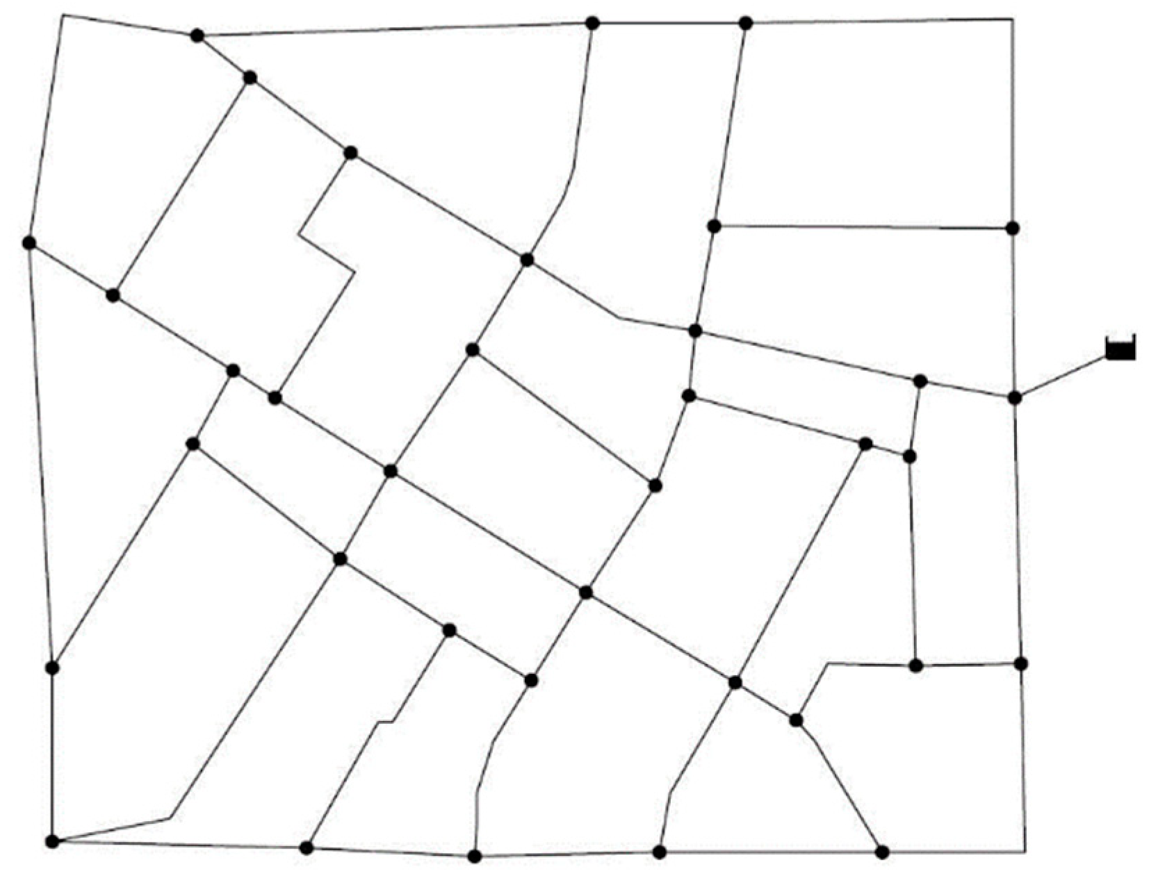
Figure 1. Water distribution network.
Water 15 03119 g001
Figure 2. The challenge of the network is solved by employing arcs whose widths are directly related to the sizes of the circles they connect. Unnumbered pipes have a 0.06 m internal diameter.
Water 15 03119 g002
Table 1. Elevation (meters) and water demand (m3/s).
i e l e v ( i ) d e m ( i )
165.150.00049
264.400.00104
363.350.00102
462.500.00081
561.240.00063
665.400.00079
767.900.00026
866.500.00058
966.000.00054
1064.170.00111
1163.700.00175
1262.640.00091
1361.900.00116
1462.600.00054
1563.500.00110
1664.300.00121
1765.500.00127
1864.100.00202
1962.900.00188
2062.830.00093
2162.800.00096
2263.900.00097
2364.200.00086
2467.500.00067
2564.400.00077
2663.400.00169
2763.900.00142
2865.650.00030
2964.500.00062
3064.100.00054
3164.400.00090
3264.200.00103
3364.600.00077
3464.700.00074
3565.430.00116
3665.900.00047
Table 2. The diameter of each pipe (meters) and the cost per meter (e/m).
r 𝒟 e , r 𝒞 e , r
10.06019.8
20.08024.5
30.10027.2
40.12537.0
50.15039.4
60.20054.4
70.25072.9
80.30090.7
90.350119.5
100.400139.1
110.450164.4
120.500186.0
130.600241.3
Disclaimer/Publisher’s Note: The statements, opinions and data contained in all publications are solely those of the individual author(s) and contributor(s) and not of MDPI and/or the editor(s). MDPI and/or the editor(s) disclaim responsibility for any injury to people or property resulting from any ideas, methods, instructions or products referred to in the content.