Article

Groundwater Level Prediction with Deep Learning Methods

1
Department of Hydraulic and Ocean Engineering, National Cheng Kung University, No. 1 University Road, Tainan 701, Taiwan
2
UNESCO-IHE, Westvest 7, 2611 AX Delft, The Netherlands
*
Author to whom correspondence should be addressed.
Water 2023, 15(17), 3118; https://doi.org/10.3390/w15173118
Submission received: 22 July 2023 / Revised: 20 August 2023 / Accepted: 28 August 2023 / Published: 30 August 2023
(This article belongs to the Section Hydrogeology)

Abstract

:
The development of civilization and the preservation of environmental ecosystems are strongly dependent on water resources. Typically, an insufficient supply of surface water resources for domestic, industrial, and agricultural needs is supplemented with groundwater resources. However, groundwater is a natural resource that must accumulate over many years and cannot be recovered after a short period of recharge. Therefore, the long-term management of groundwater resources is an important issue for sustainable development. The accurate prediction of groundwater levels is the first step in evaluating total water resources and their allocation. However, in the process of data collection, data may be lost due to various factors. Filling in missing data is a main problem that any research field must address. It is well known that to maintain data integrity, one effective approach is missing value imputation (MVI). In addition, it has been demonstrated that machine learning may be a better tool. Therefore, the main purpose of this study was to utilize a generative adversarial network (GAN) that consists of a generative model and a discriminative model for imputation. Although the GAN could not capture the groundwater level endpoints in every section, the overall simulation performance was still excellent to some extent. Our results show that the GAN can improve the accuracy of water resource evaluations. In the current study, two interdisciplinary deep learning methods, univariate and Seq2val (sequence-to-value), were used for groundwater level estimation. In addition to addressing the significance of the parameter conditions, the advantages and disadvantages of these two models in hydrological simulations were also discussed and compared. Regarding parameter selection, the simulation results for univariate analysis were better than those for Seq2val analysis. Finally, univariate was employed to examine the limits of the models in long-term water level simulations. Our results suggest that the accuracy of CNNs is better, while LSTM is better for the simulation of multistep prediction. Therefore, the interdisciplinary deep learning approach may be beneficial for providing a better evaluation of water resources.

1. Introduction

Due to its geographical and hydrological environment, Taiwan has suffered from insufficient water resources [1]. An insufficient supply of surface water is conventionally supported with groundwater. However, groundwater is a resource that accumulates over many years. Furthermore, excessive extraction of groundwater leads to land subsidence [2,3,4,5,6,7,8]. Hence, there remains a need to perform long-term water management. To be able to effectively allocate water resources, groundwater levels must be accurately predicted.
During the process of data collection, data may be missing due to various factors. Therefore, dealing with missing data is a challenge that needs to be overcome in any research field. To maintain data integrity, the missing value imputation (MVI) method is often chosen as a solution. Many missing value imputation methods lack validation. Thus, many studies have utilized machine learning techniques, simulating the learning process of neural networks, to impute missing values. Results have shown that model-based machine learning methods are more effective. Currently, artificial neural networks (ANNs) are widely used in hydrological research as an important tool for groundwater management. However, in recent decades, the thrust of artificial intelligence has gradually changed from machine learning to deep learning [9]. Missing data is a problem that must be overcome in any research field. In recent years, research on using machine learning to supplement missing value imputation has gradually increased. In 2011, Buuren et al. [10] applied the MICE framework to a machine learning model and confirmed that the hybrid framework incorporated into the deep learning model can increase accuracy. Stekhoven et al. [11] established MissForest with a machine learning framework, labeled the data as a test set and training set, and achieved good simulation results.
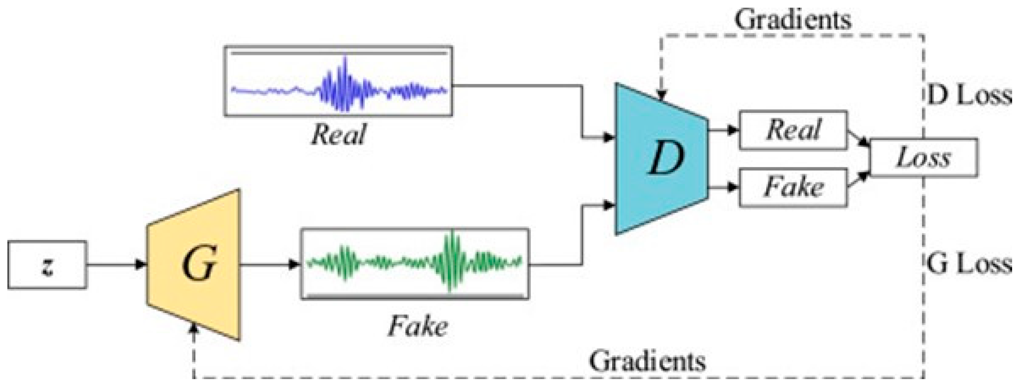
Imputation models can be divided into discriminative models and generative models. Candes et al. [12] used matrix completion to restore a low-rank matrix identification model but could not handle sparse matrices with missing data. The denoising autoencoder (DAE) proposed by Vincent et al. [13] is a generative model. Although it has the ability to resist noise, it cannot handle data with a large amount of information. To solve the disadvantages of the two categories, in 2014, Goodfellow et al. [14] created the generative adversarial network (GAN), combining properties of the generative model and discriminative model, as shown in Figure 1. The two networks compete against each other to achieve Nash equilibrium, which greatly reduces the amount of data needed. It is the first network architecture capable of unsupervised deep learning.
Data missingness can be categorized into three types based on likelihood: missing completely at random (MCAR), missing at random (MAR), and missing not at random (MNAR). In the case of groundwater level data, they fall under the MCAR category. This aligns with the focus of GAIN [15], which is specifically designed for this type of data. The study employs a framework with a priors (hints) mechanism to address the missing value situation in groundwater hydrology.
Figure 1. GAN model (source: Pan et al. [16]).
Water 15 03118 g001
In the past, predecessors utilized widely applied physical models such as the Soil and Water Assessment Tool (SWAT) [17,18,19] and the modular three-dimensional groundwater flow model (MODFLOW) [20,21] to predict groundwater levels. In many cases, the lack of physical awareness of implicated processes might create problems in finding applicable models [22], and two additional barriers are the significant computational demands and the requirement for extensive hydrogeophysical data [23,24]. As a result, the modeling process remains fraught with uncertainty and challenges [25]. Moreover, under comparable simulation conditions, the modeling performance of ANNs surpasses that of MODFLOW [26]. Over the last decades, ANNs have sparked growing interest among researchers in various water resource issues and have obtained encouraging results [27,28,29,30], and numerous studies have employed various soft computing techniques such as a self-organizing map (SOM), an adaptive neuro-fuzzy inference system (ANFIS), GMDH, a supervised committee machine with artificial intelligence (SCMAI), boosted regression trees (BRT), and Bayesian networks (BNs) to simulate time series. For instance, ANNs have been utilized for predicting groundwater level time series [31,32,33,34,35], estimating hydrogeological groundwater contamination, comprehending inter-annual dynamics of recharge [36,37,38], and capturing the influence of controlling factors on these processes [39,40].
Research on time series prediction began with regression equations, such as the autoregressive–moving average (ARMA) and autoregressive integrated moving average (ARIMA) models, which are the most basic modeling approaches [41,42]. However, achieving high-precision predictions for nonlinear data using complex models is challenging. Machine learning methods, on the other hand, can construct nonlinear models based on extensive historical data. Through iterative training and learning approximations, they can provide more accurate predictions compared with traditional statistical models. Typical methods include support vector machines (SVMs) [43], ANNs, and ensemble learning methods [44,45]. However, these aforementioned techniques often lack the effective handling of dependencies between variables, leading to limited predictive effectiveness [46].
Subsequently, LeCun [47] confirmed that deep learning can effectively mitigate the interference of outliers during the process of data feature extraction, thereby leading to a significant enhancement in technical capabilities across various domains [48,49]. As we know, in 1982, Hopfield [50] published a recurrent neural network (RNN) for sequence data, laying the foundation for deep learning models, and is often seen as the most efficient method of time series prediction. However, RNNs have vanishing gradients and exploding gradients in the process of backward transmission and cannot memorize long sequences. To improve the RNN problem, Hochreiter and Schmidhuber [51] developed long short-term memory (LSTM) to improve memory function, which is considered one of the most advanced methods for addressing time series prediction problems [52]. Hence, this study incorporated LSTM to simulate daily water levels.
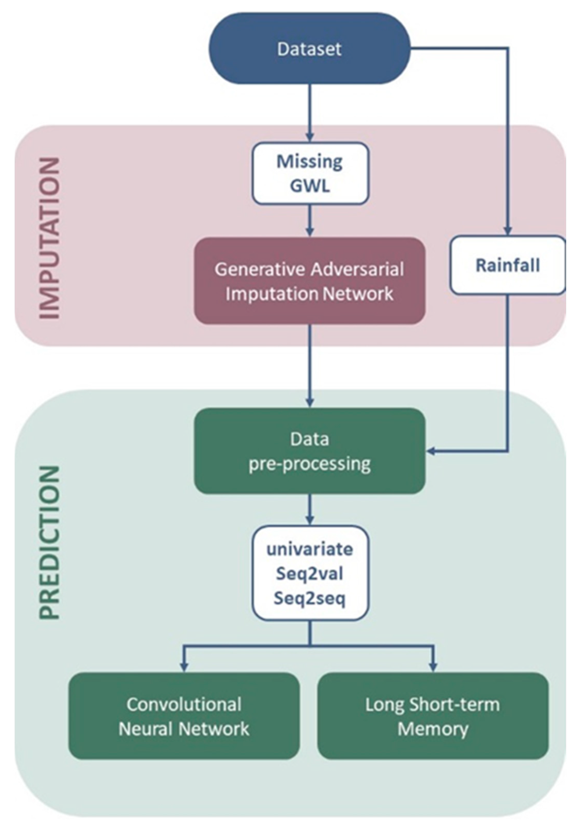
In addition, LeCun et al. [53] combined the neocognitron to propose a convolutional neural network (CNN) and then applied the model to a one-dimensional CNN with Bengio et al. [54]. Learning features from sequence data gradually allows the network to achieve excellent performance in signal data and natural language. A CNN mainly extracts spatial information from image-like data, while LSTM was developed for sequence data. In this study, LSTM and a CNN were used to simulate water levels, and the differences between the two methods were compared. This study is expected to reduce the limitations of sequence data research methods and provide more possibilities for water resources research. Therefore, to address the problem of missing hydrological observation data, the purpose of the present study is to use a GAN for imputation. Complete hydrological data can improve the accuracy of groundwater level prediction. Accordingly, the performance of groundwater level prediction was compared using two interdisciplinary methods. One is the LSTM model specially developed for sequence data, while the second model is a CNN, which is good at processing image information. Figure 2 shows the flow of the entire research.

2. Materials and Methods

2.1. Case Study

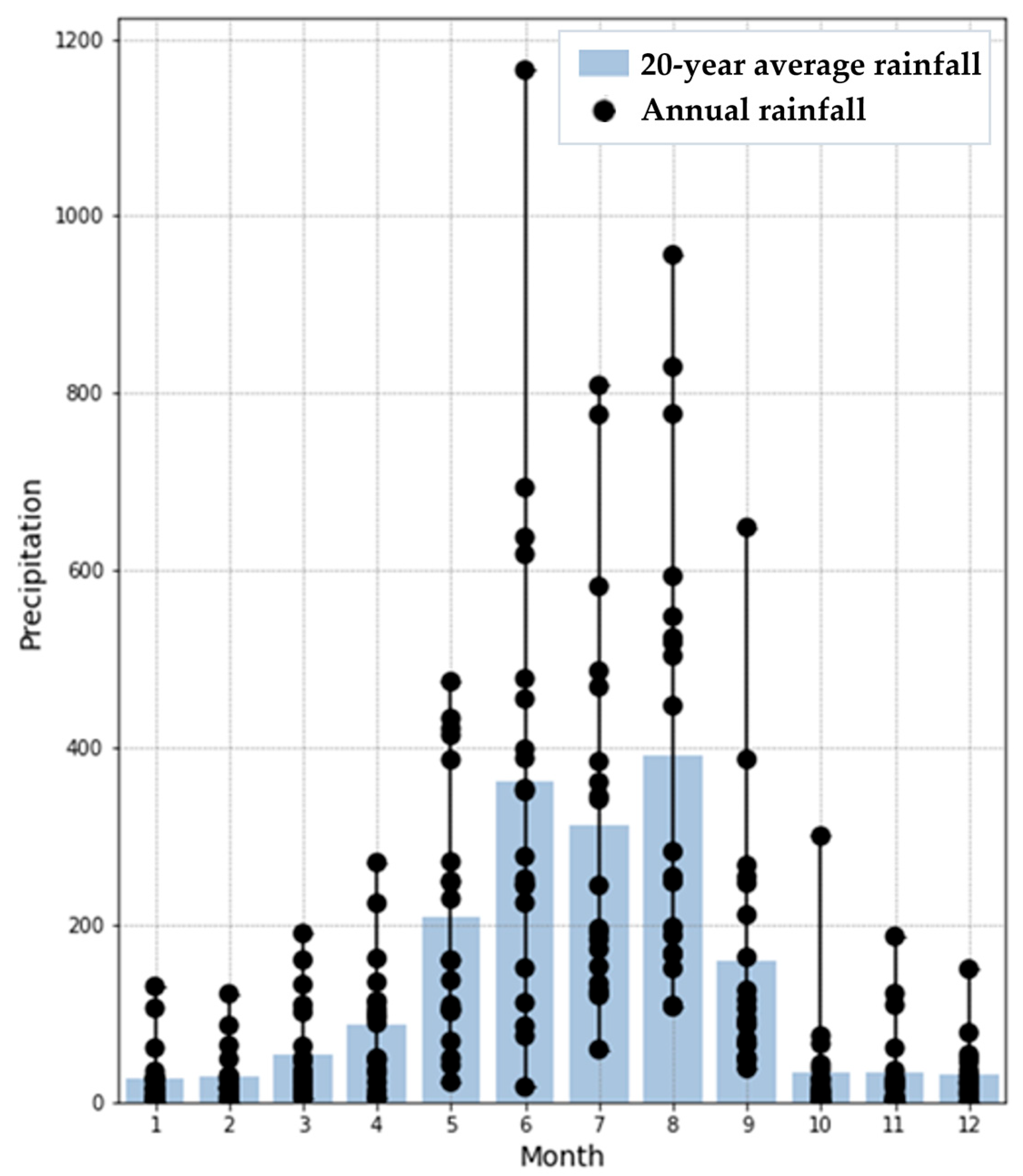
The research area was in the Choushui River basin, the second-largest basin area in Taiwan. The slope increases from west to east, and the mainstream is 186.6 km long, making it the longest river in Taiwan. The elevation of the basin is approximately 0–100 m, the terrain is flat, and the groundwater subdivision contains rich water resources. The area is as large as 3156.9 square kilometers, which is the second-largest basin area in Taiwan. The mainstream comes from between the main peak and the east peak of Mount Hehuan, which is approximately 3200 m above sea level. Due to the large terrain changes, the information from the rainfall station of the Central Weather Bureau shows that the spatial distribution of annual rainfall decreases when moving from mountainous areas to the coast. The eastern side has steep mountains and abundant rainfall, while the western coast has less rainfall. Geographically south of the Tropic of Cancer, the Choushui River is affected by ocean currents and thus has a tropical marine climate, resulting in an extremely uneven spatial and temporal distribution of rainfall. Figure 3 shows the monthly average rainfall in the Choushui River. However, the temporal distribution of rainfall throughout the year is strongly heterogeneous. On average, 75% of total annual rainfall falls between May and September in the wet season (or the high-flow period), while October to April of the next year is the dry season (or the low-flow period), with only 25% of annual rainfall. Coupled with the impact of extreme climates in recent years, the difference between abundance and drought is particularly obvious.
The Central Geological Survey Report [55] noted that the strata in the Choushui River Basin are long and narrow from north to south and slightly westward in an arc-shaped distribution. According to soil properties and water content characteristics, it is divided into fan top, fan center, and fan tail [56]. The fan top is composed of unconsolidated sediments, with good strength and water permeability, and is easily recharged with surface water. It is an area rich in groundwater resources. The shallow layer in the central fan area is composed of coarse medium sand mixed with silt sand with well-developed pores and is the main aquifer. The deep layer is mostly a clay layer, and the thickness of the water-blocking layer increases gradually, and the denser layer leads to poor water permeability. From the center of the fan to the tail of the fan belongs to the middle and lower reaches of the mainstream, and the alluvial layer with a thickness of several hundred meters is formed by the alluvial flow of the river. It is mainly composed of clay and silt, and the aquifer is thinning. When one artificially overpumps the groundwater, the surface elevation is lowered, causing formation deformation and compression.
To explore the long-term groundwater variability, data collected from 2002 to 2021 by the Water Resources Agency (MOEA) were used. We knew the general situation and distribution of observation wells and detected missing 20-year long-term data. There were 63 stations with missing data [57,58]. The stations with too much missing data were eliminated, and the stations with 2~40 missing days of data were interpolated. Then, Thiessen’s polygon method was used to configure the rainfall data for observation wells, and the GAN was used to interpolate the missing values to obtain complete data.
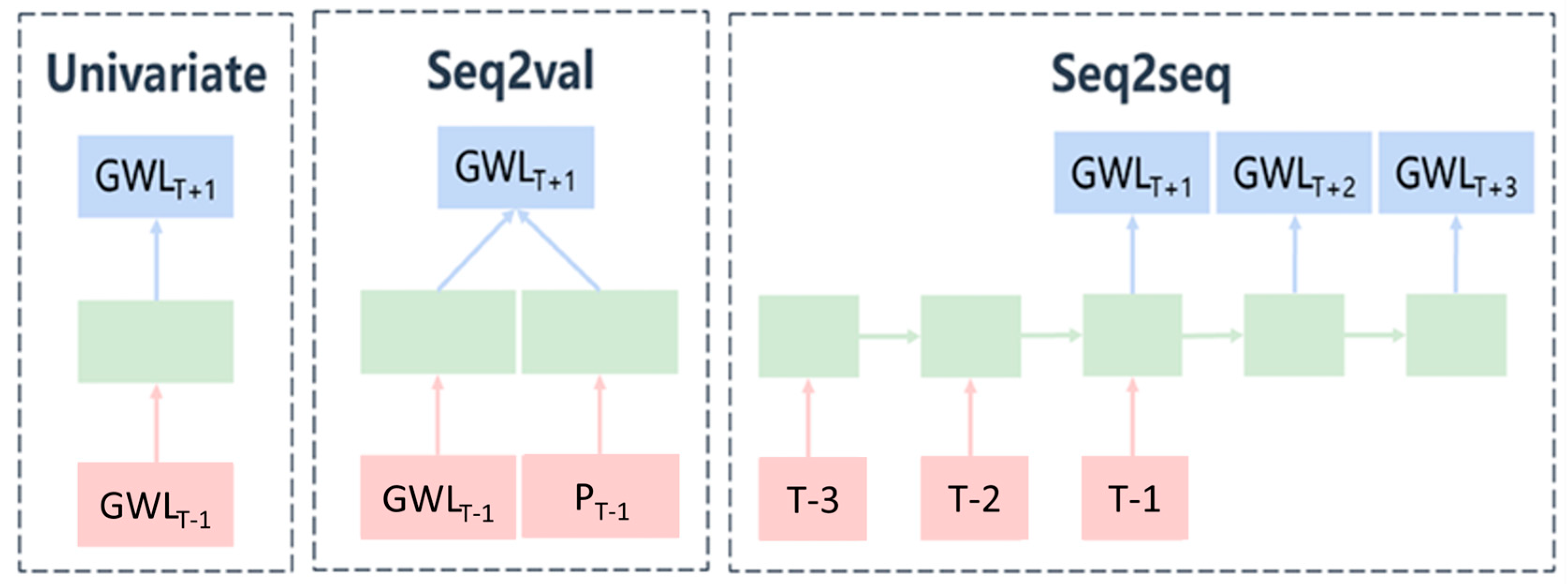
Due to the high autocorrelation of the time series data, the univariate and Seq2val (sequence-to-value) frameworks were used to run the CNN and LSTM, respectively. We discussed the significance of the parameters and the advantages and disadvantages of the model and indicated that the two-cross-domain model can be applied to hydrology. Finally, the encoder–decoder framework proposed by Hamilton et al. [59] was incorporated to develop Seq2seq at the limit of long-term simulated water levels, as shown in Figure 4.

2.2. Methodology

To investigate the long-term groundwater variability, the measured groundwater level in the alluvial fan of the Choushui River from 2002 to 2021 was used as the examined data. First, the imputation of missing data was performed. For this purpose, five years of data were used to train the GAN. After our preliminary results were successfully verified, the missing part of the 20-year groundwater level data could be further imputed. In the current study, univariate and Seq2val were employed using the groundwater level and rainfall as hydrological parameters, which were inputted into the CNN and LSTM models, respectively. Then, the meaning of the parameters as well as the pros and cons of the models were discussed. Finally, the encoder–decoder was incorporated to explore the limit of the long-term simulated groundwater level in Seq2seq.

2.2.1. Water Level Prediction Data Preprocessing

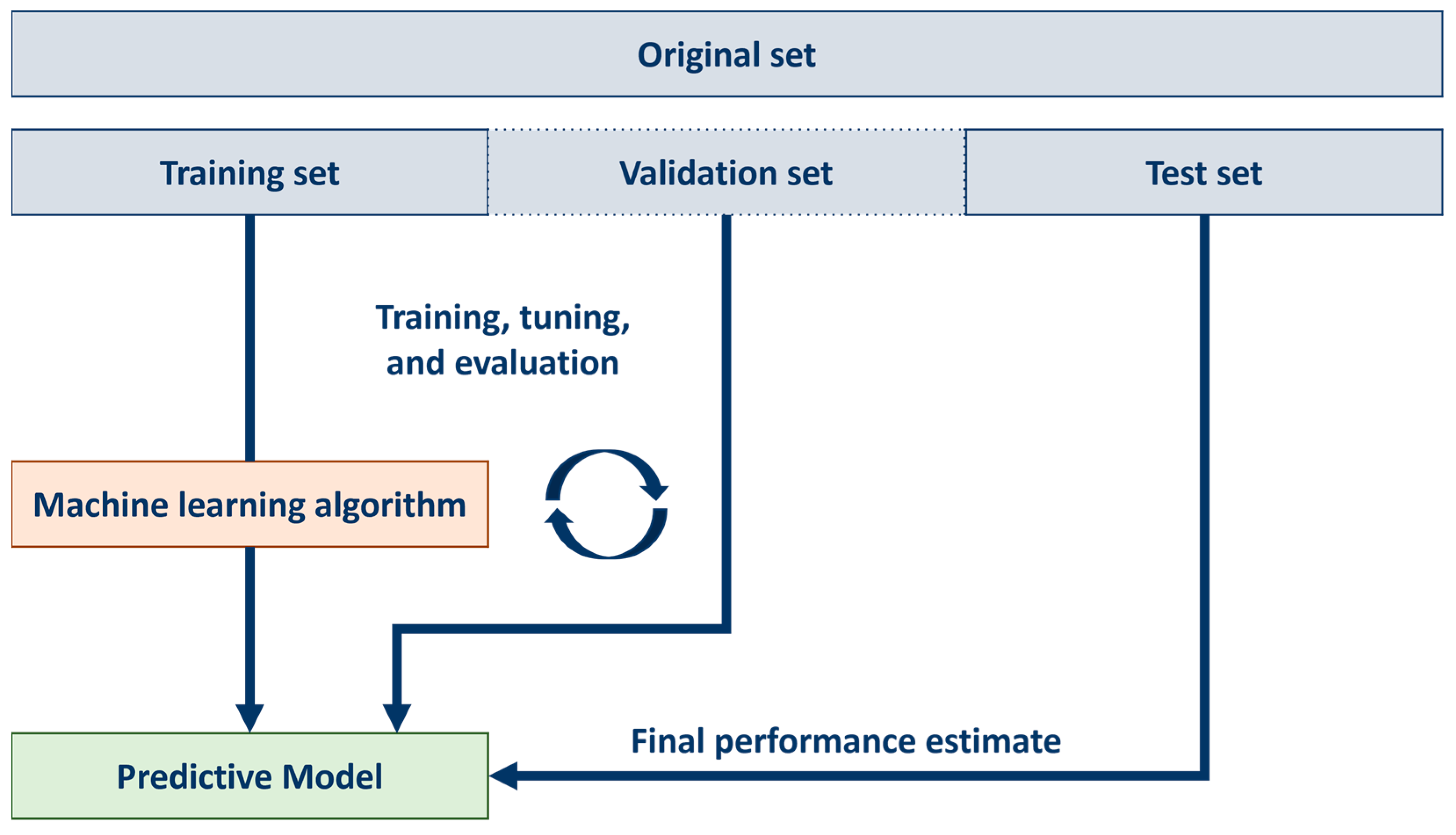
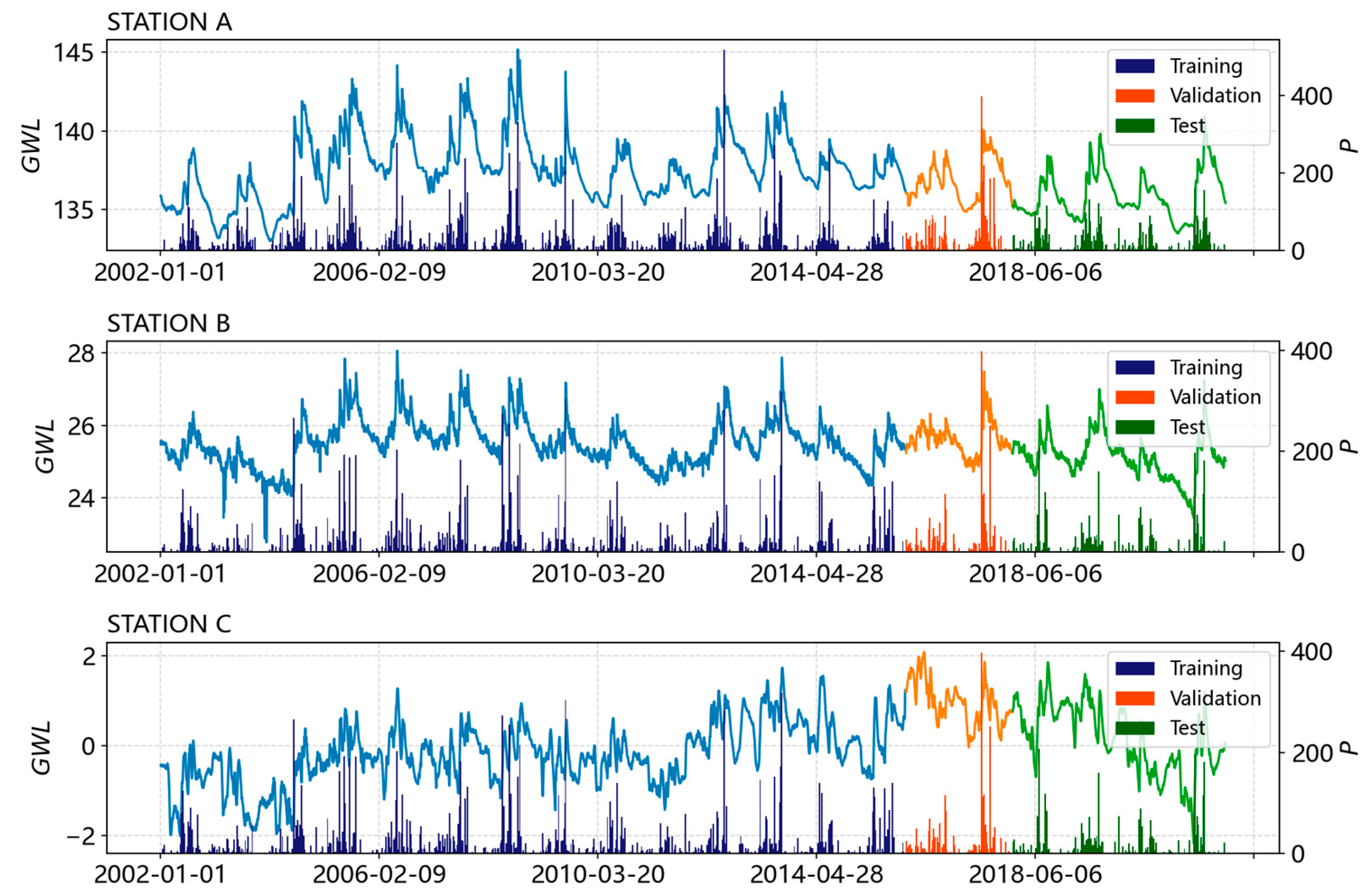
To supervise the model to achieve a reasonable balance, the holdout method [60] was used to divide the data into three parts according to the following ratio: 70% for the training dataset (2002~2015), 10% for the validation dataset (2016~2017), and 20% for the test dataset (2018~2021), as shown in Table 1, Figure 5 and Figure 6.
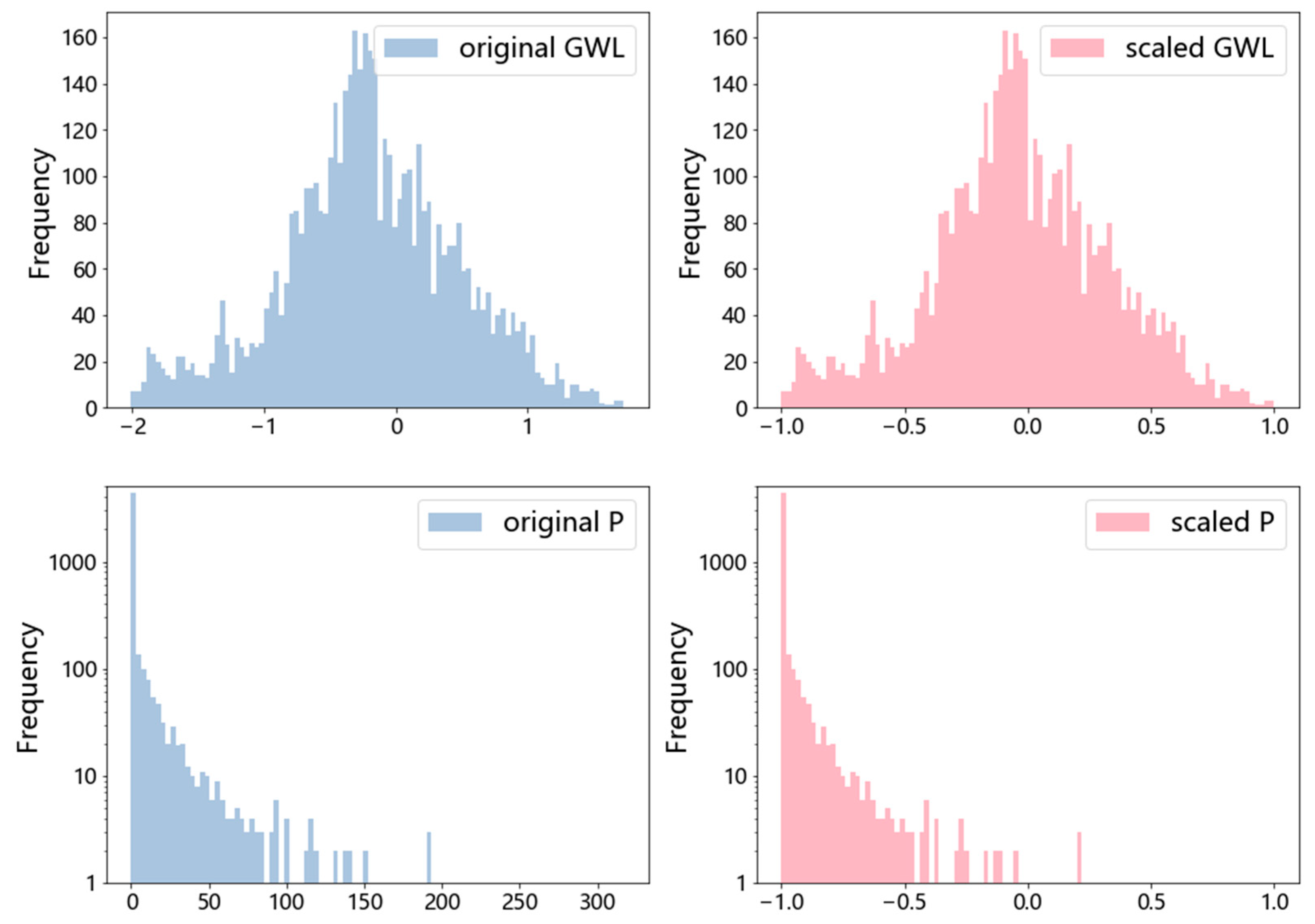
X n o m = X μ X m a x X m i n [ 1 , 1 ]
The research parameters were the daily groundwater level and daily rainfall, and the representativeness and values of the two were completely different. Therefore, to ensure that the model training could be driven normally, the data had to be preprocessed via normalization, as shown in Figure 7.

2.2.2. Generative Adversarial Network

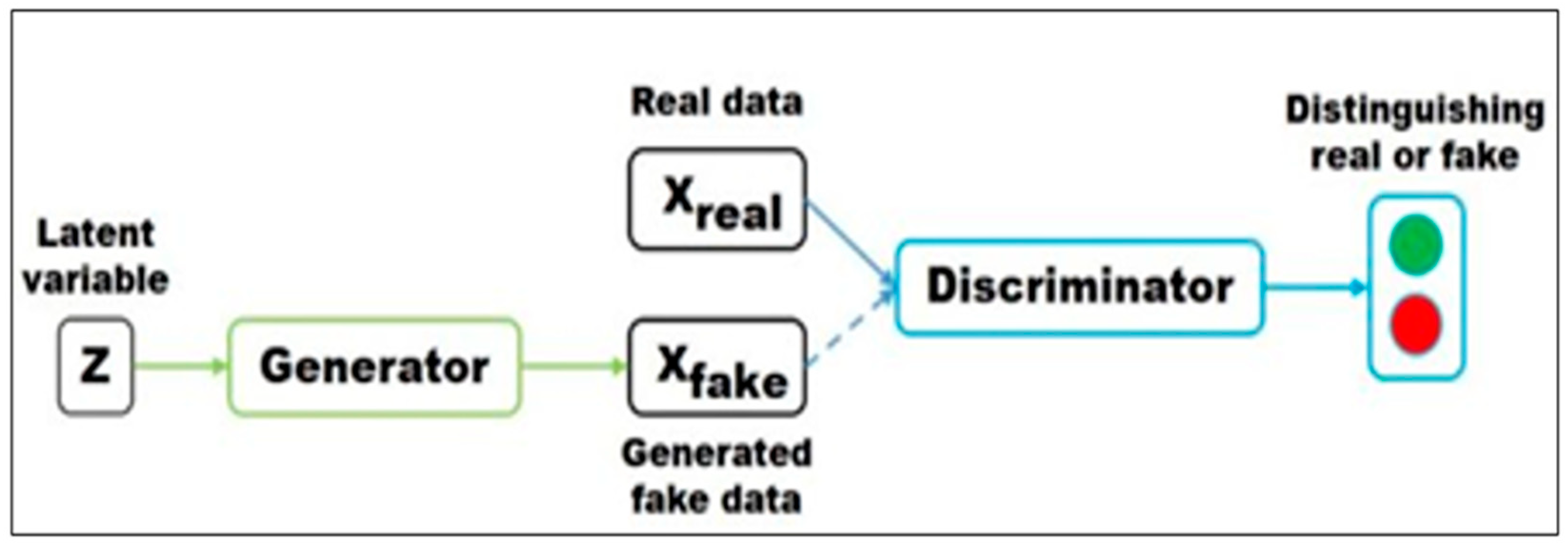
The generative adversarial network (GAN) was proposed by Goodfellow et al. [14] in 2014. It is the first deep learning application that enables unsupervised learning. Figure 8 shows that it learns the distribution of data in such a way that the discriminating network and generative network compete with each other without relying on any assumptions. A GAN generates samples using forward propagation to reduce computational costs and stops upon reaching Nash equilibrium. Research has incorporated cueing mechanisms to reinforce the process [15]. We used the self-defined random variable H M = m to prompt the discriminating network and train the best neural network (NN).
L = E log P F = r e a l   | X r e a l + E log P F = f a k e | X f a k e
Random noise (z) is sampled from the latent space following a Gaussian distribution. The generator G produces Xfake, which approximates real values, while both Xfake and Xreal are used as inputs to the discriminator network. The training objective function is a binary classification task aimed at distinguishing between Xreal and Xfake.

2.2.3. Long Short-Term Memory

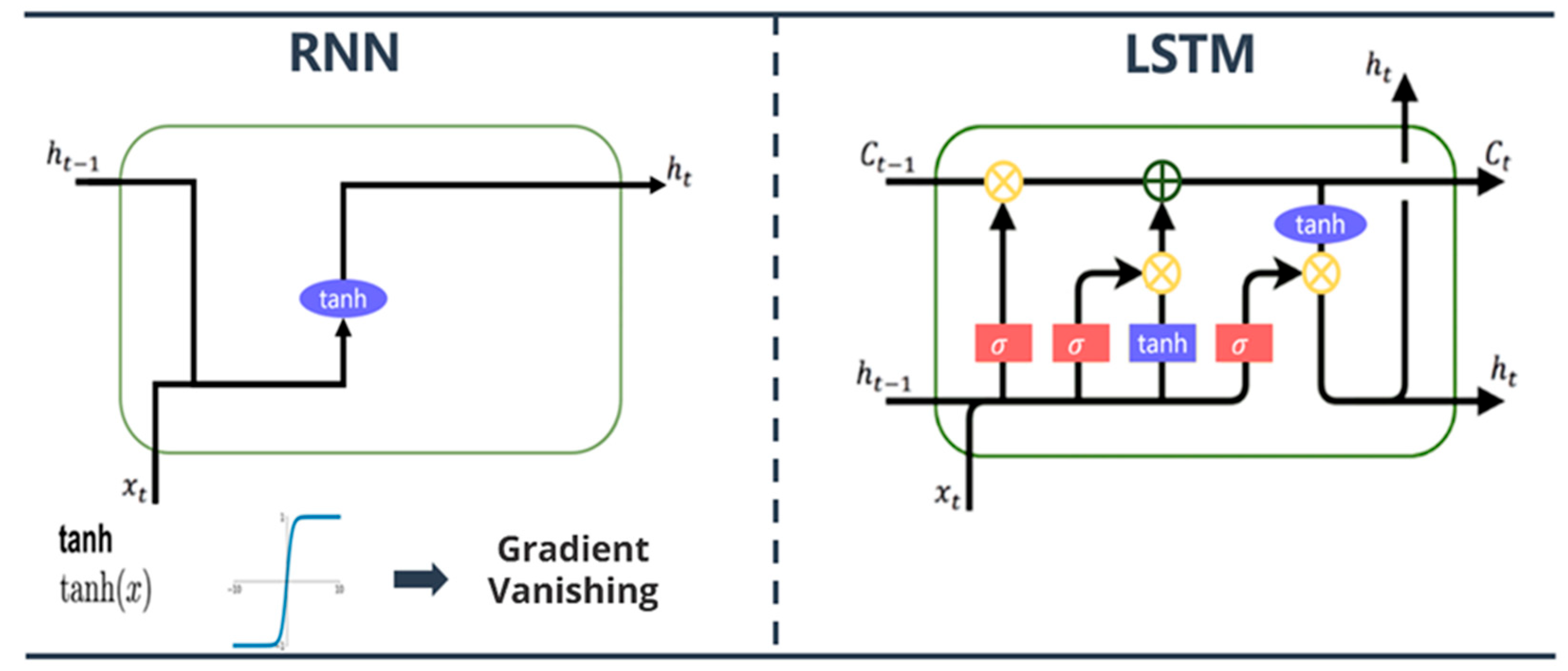
In 1997, Hochreiter and Schmidhuber [51] proposed LSTM based on the RNN and added cell states to improve the memory function, as shown in Figure 9. They increased the long-term dependence of the model and successfully solved the defects of RNN gradient vanishing and gradient explosion. LSTM is mainly composed of three stages: an input gate, an output gate, and a forget gate. Four kinds of information are obtained via splicing training with the current input and the previous transfer state. Among them, f t , i t , o t are normalized with sigmoid to [0, 1], while C ~ t is normalized with the Tanh activation function to [−1, 1] to assist memory update and storage.

2.2.4. Convolutional Neural Network

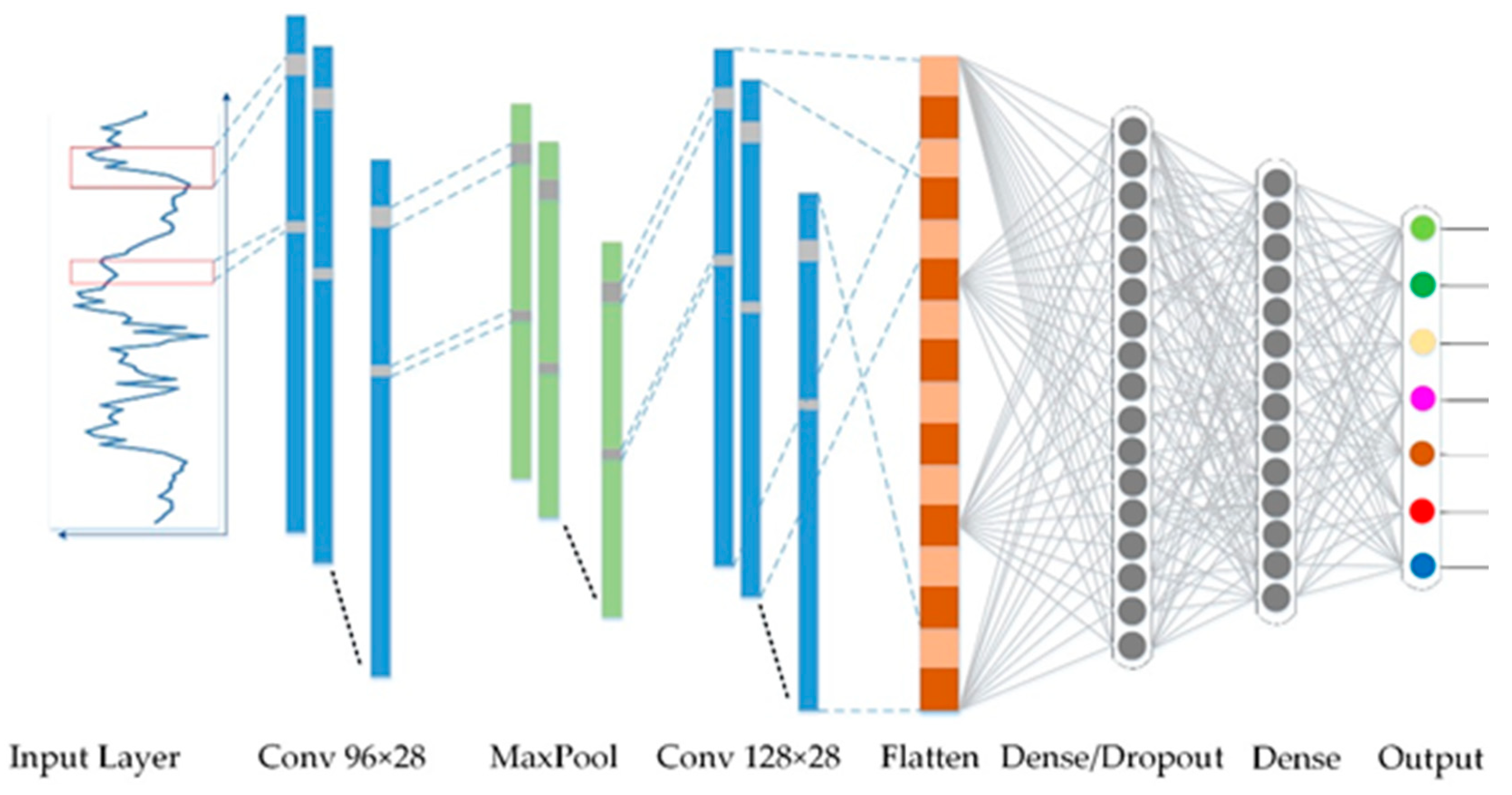
In 1989, LeCun et al. [53] proposed the CNN infrastructure LeNet-5, which mimics the neuron structure of the human visual cortex. It was based on the neocognitron proposed by Japanese scientist Fukushima et al. [61] in 1980, laying the foundation for CNNs. Through the continuous complexity of the model and the maturity of hardware technology, CNNs became the ImageNet champion in 2012. LeCun and Bengio [54] developed a one-dimensional (1D) CNN to learn features from segment sequence data, making the scope of the CNN more diverse. Whether a CNN is 1D, two-dimensional (2D), or three-dimensional (3D), it follows the same method and characteristics, and the only difference is in the method of extracting features, as shown in Figure 10. Figure 11 shows that a CNN mainly consists of convolutional layers, pooling layers, and fully connected layers. A CNN uses filters to extract information features and convolves data with sliding windows to reduce computational costs. The weights are computed using the chain rule and updated with backpropagation. This enables sequence data to preserve the location information of features and has the advantage of full-value sharing.

2.2.5. Objective Function

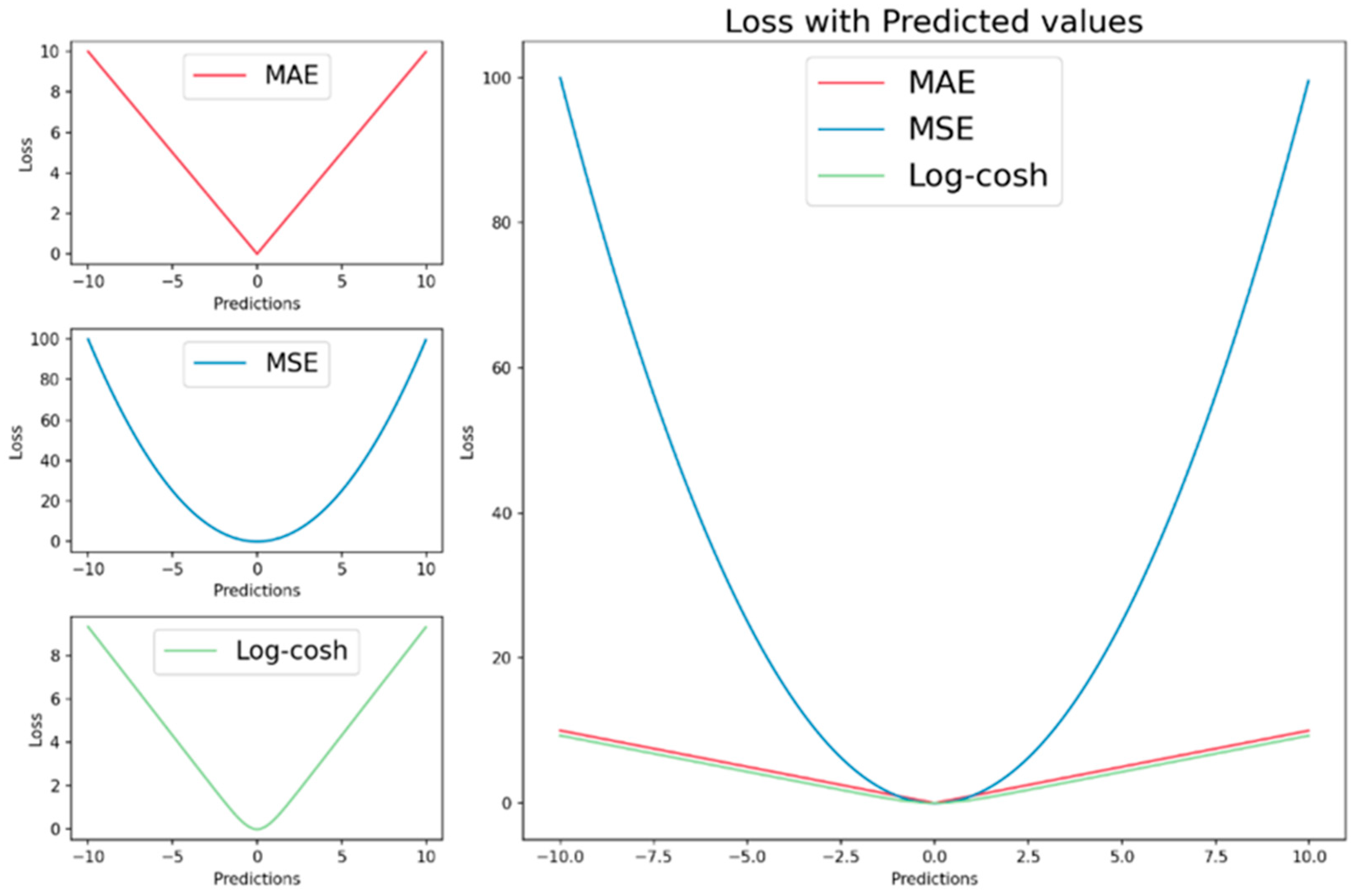
Written in Python version 3.9.5, packages such as NumPy, pandas, scikit-learn, and Matplotlib were used to perform basic operations. TensorFlow and Keras were also used for data imputation, training, and simulation. The most common mean absolute error (MAE), mean square error (MSE), and log-cosh metrics were selected for loss function screening, as shown in Figure 12. Finally, to detect whether the model exhibited underfitting or overfitting, we used MAE, RMSE, and R2 as evaluation indicators.
  • MAE
The mean absolute error (MAE) is a linear function that solely measures the average value of modeling errors. It is less susceptible to the influence of outlier data points, making it suitable for scenarios where anomalies are treated as damaged data. However, a drawback is that its gradient remains constant, even when the loss value is small, and the gradient remains large, which can hinder neural network learning and potentially lead to missing the optimal point.
M A E = 1 n i = 1 n y i y ^ i
  • MSE
Mean squared error (MSE) is a regression loss function, and the gradient changes accordingly based on the increase or decrease in the loss. MSE is also sensitive to outliers, which can lead to rapid amplification. It is suitable for datasets where outliers represent significant anomalous situations.
M S E = 1 n i = 1 n ( y i y ^ i ) 2
  • Log-cosh loss
The advantages of Log-cosh, which combines the benefits of MSE and MAE, include its tendency to converge near the optimal value as gradients progress and its robust handling of outlier values. However, log-cosh may not be a perfect fit for this specific dataset due to gradient issues arising from significant deviations in the modeled values.

3. Results

3.1. The Results of Imputation

3.1.1. Hyperparameter Settings of GAN

The hyperparameters of the GAN were the result of repeated adjustments. The model only set the batch size and number of iterations. Adam in Table 2 was controlled by Alpha and the Hint rate, and the nonlinear relationship was added using ReLU. The main objective of this research’s target function was to minimize the loss function, where the model returns the function difference to assist in gradually adjusting the parameters. A smaller function value indicates that the simulated values are closer to the real values. Finally, the error was returned by the MSE, and the weight parameters were gradually adjusted.
  • Adam
Adam is one of the optimization methods used for model optimization and is an extension of the gradient descent optimization algorithm. It was proposed by Kingma and Ba in 2015 [63] and has been widely applied in various deep learning applications. Compared with the traditional gradient descent method, which uses a fixed learning rate, Adam can adjust the learning rate adaptively and remember the previous gradient states. Adam performs well in both linear and non-linear functions and exhibits advantages over other adaptive learning methods. It also requires less memory and is computationally efficient, making it well suited for large datasets. Therefore, in this study, Adam was selected as the optimization tool.
  • ReLU
Rectified linear units (ReLU) is a piecewise linear function widely used in deep learning applications due to its ability to address the vanishing gradient problem. As indicated in Equation (2), ReLU only activates input values that are greater than zero. This characteristic accelerates convergence and better aligns with the activation patterns observed in the human brain.
f ( x ) = max ( 0 , x )

3.1.2. Imputation Results

The research data were classified as “MCAR” (missing completely at random). In the literature on missing value imputation, only 10.8% of the articles imputed more than 50% of the missing values. To evaluate the stability and limits of the GAN, the data used a matrix of size [2192 × 46] composed of 46 stations with no missing records in 2015–2020. To imitate missing data scenarios, complete data can be randomly generated with missing rates of 10%, 20%, and up to 90%. Additionally, consecutive missing values for a duration of 2 to 30 days can be introduced, and then imputation techniques can be applied to fill in the missing values.
Figure 13 presents the imputation results using the GAN, evaluated based on the RMSE. The blue area indicates a good imputation performance, while the boundary between the white and red areas represents the limit of data imputation in this study. This result was used as the criterion for selecting imputed stations. Stations with missing data falling within the white or red areas were directly excluded from the imputation process and were not considered for imputing missing values.

3.1.3. Practical Imputation Case Discussion

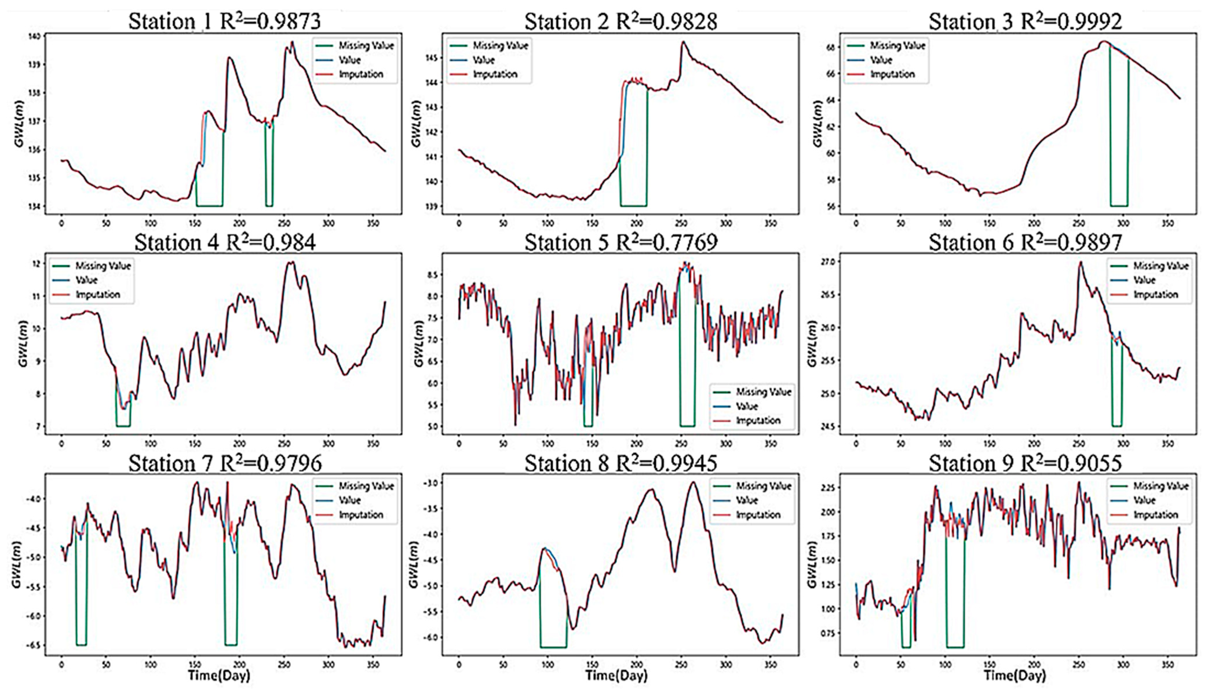
Water levels vary by geographic location. Figure 14 shows that the water level at the top of the fan (Stations 1–3) is high, the curve is smooth, and the simulation results are excellent. However, the water level significantly curves at the center (Stations 4–6) and tail (Stations 7–9) of the fan fluctuate, and the difference in local changes makes the interpolation error larger. In particular, Station 5 and Station 9 have the most drastic changes, and the peaks do not fit well, resulting in poor performance, as captured by the evaluation indicators. However, there is still an overall trend, so the feasibility of the model can be determined.
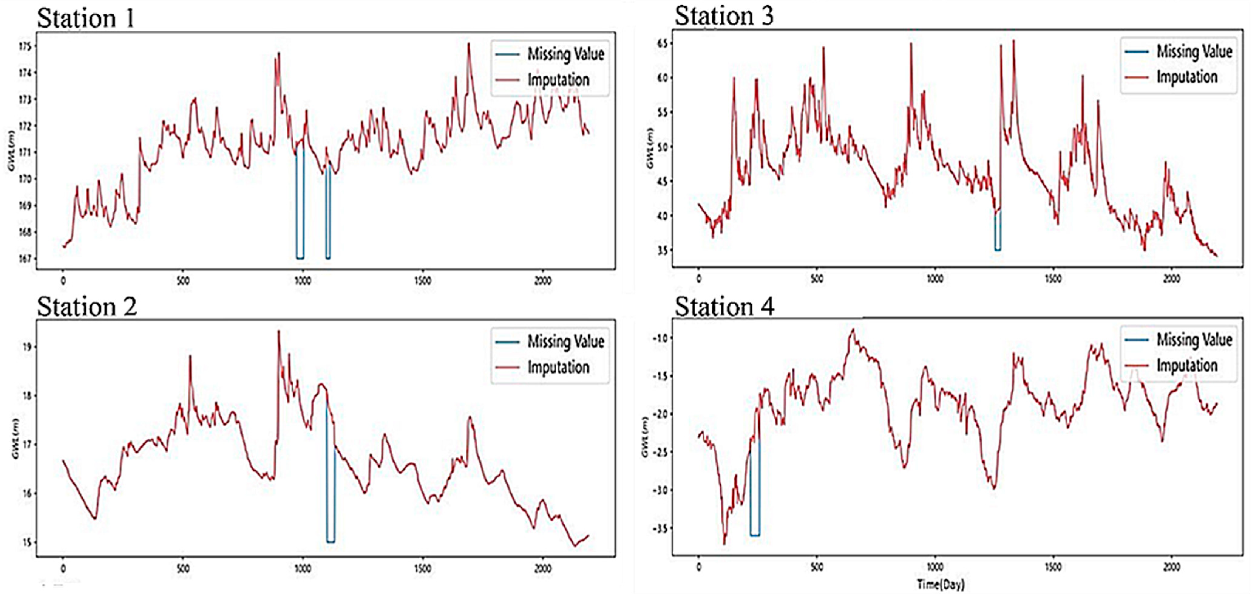
Imputation was performed on the actual missing data. Figure 15 shows the serial trend can be captured in the smooth segment and that Station 2 is consistent with the normal regression segment. Each station was affected by different external factors, resulting in different shocks. However, since the model is trained with Gaussian random noise, it has a certain ability to resist noise. There are sudden rises and falls in the steep rising section of the daily water level. The water level of Station 3 rises gently and then is straight until the peak, which shows that the reaction of raw water is slightly slower. However, the series still maintains a stable change, which can be used to identify the overall trend.

3.2. Prediction Results

3.2.1. Hyperparameter Settings of CNN and LSTM

We referenced callbacks to monitor data changes and set EarlyStopping. When overfitting occurred or the model index did not improve and the convergence was too slow, the training was automatically terminated. When there was no abnormality in the training process, it automatically judged and stopped at the best epoch. Finally, ModelCheckpoint retained the best parameters to improve the model setting adjustments. Hyperparameter Settings of CNN and LSTM are shown in Table 3, Table 4, Table 5 and Table 6.

3.2.2. Results of Prediction

This section presents the results of the CNN and LSTM models. Root-mean-square error (RMSE), mean absolute error (MAE), correlation coefficient (R2), scatter index (SI), and BIAS were used to assess the performance of the models. The formulas for these statistical parameters have been provided in the literature [64,65,66].
  • Univariate and Seq2val
There was no significant difference between the simulated water levels of the CNN and LSTM, and the endpoint values were accurately simulated. The overall performance was excellent, and the R2 values of the four models were all as high as 0.99 in Table 7. The accuracy of the CNN was not lower than that of LSTM, which means that the CNN does have strong potential for the prediction of one-dimensional data. Seq2val performed worse than univariate, indicating that the methods perform poorly on multivariate data. It is speculated that due to the large difference in parameter values, the weight of rainfall was too large, resulting in a slight shift in the RMSE.
  • Seq2seq
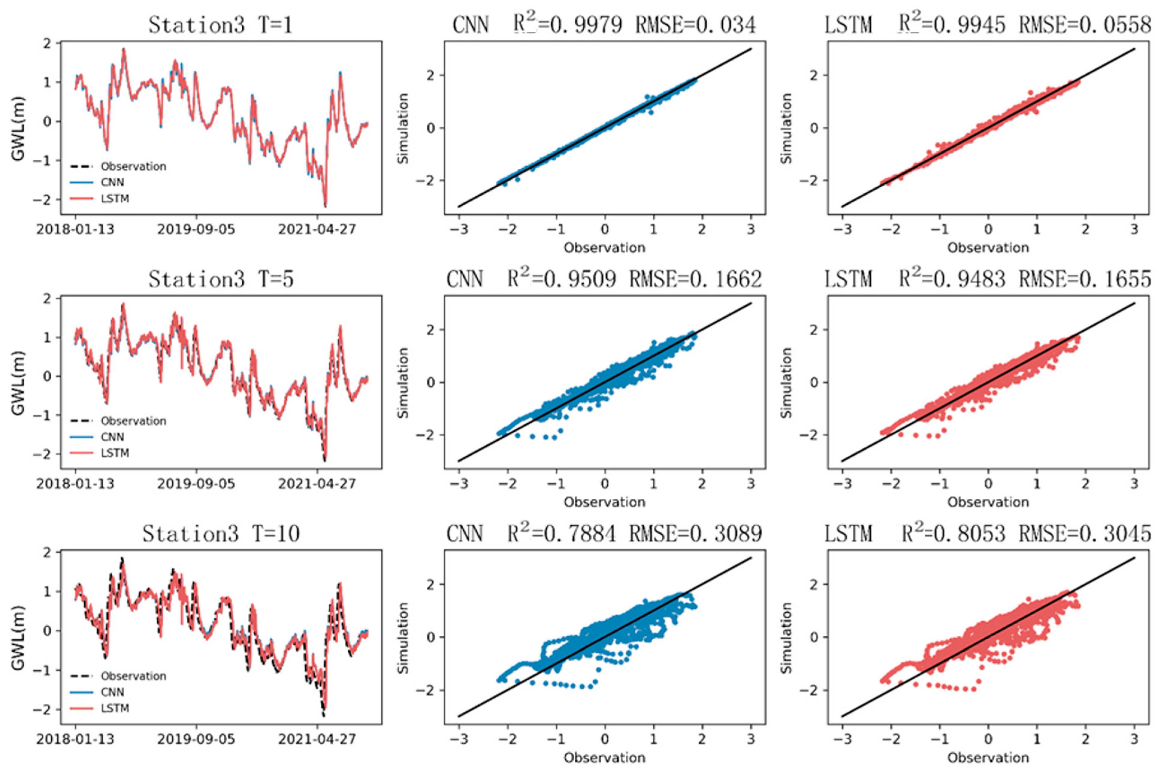
Since the above results indicate better performance using univariate analysis, these data were used to test the limits of the simulation. Multistep prediction of the CNN and LSTM with the Seq2seq framework was carried out. The peak value was slightly shifted within T = 5, but the R2 was as high as 0.95 in Table 8, which indicated good performance. Although the R2 of T = 5–7 was above 0.9, the RMSE was not excellent. It is speculated that where the curve changed sharply, the endpoint simulation was slightly extreme. After T = 7, the evaluation index gradually deteriorated, and the accuracy of the CNN decreased faster than that of LSTM, indicating that LSTM is still relatively good at remembering long-term information. Overall, the simulation accuracy of both models is good, and that of the CNN is slightly better. It is confirmed that the CNN can also be used as a tool for sequence data, and it has more potential in the field of hydrology.
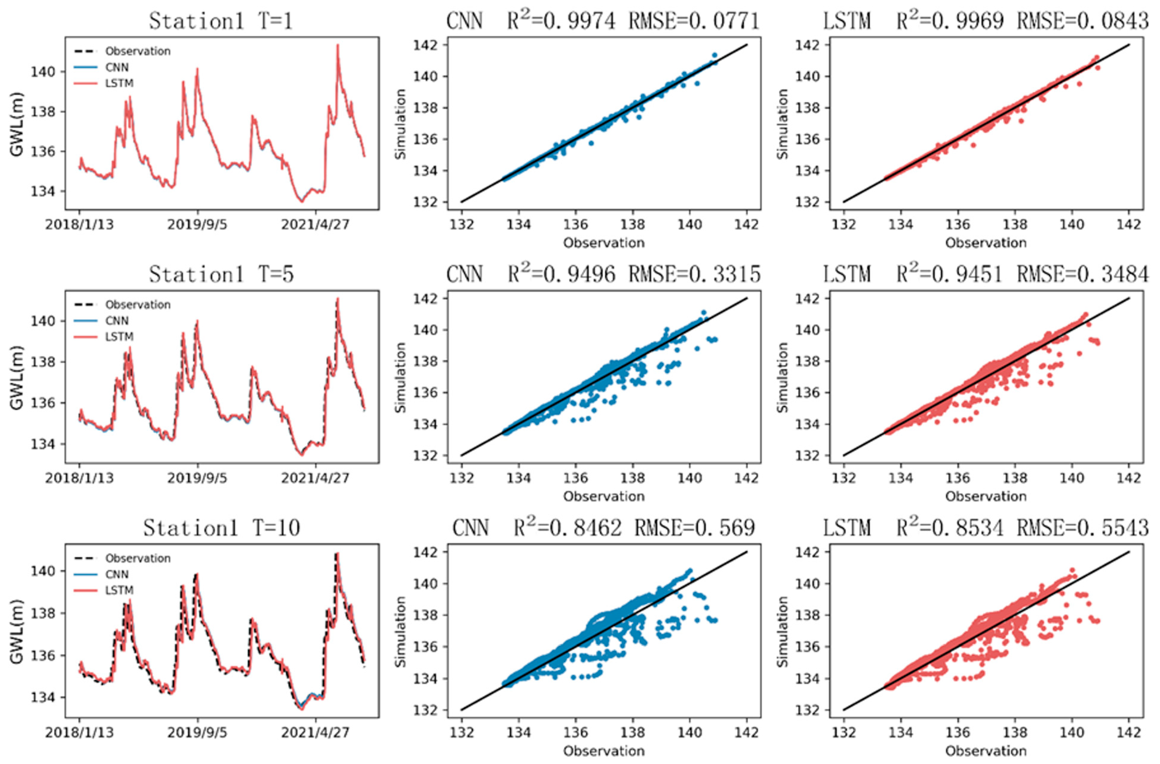
Figure 16, Figure 17 and Figure 18 show the simulation results of the three parts of the alluvial fan. T = 1 of Station 1 is in a mountainous area with a high daily water level and suffers less noise. However, Station 2, which is in the center of the fan, has more shocks, resulting in a slightly lower R2. LSTM has high accuracy on the smooth segment but has a slightly extreme phenomenon on the simulated endpoint. The CNN evaluation indices are better. However, both CNN and LSTM are suitable tools for simulating groundwater, and both R2 values are as high as 0.98 or more. T = 5 shows that the two models are worse at simulating extreme values, and there is a shift in the smoothing section, resulting in a rapid increase in the RMSE. This is especially the case for Station 2, which is more affected by noise: the simulation curve of LSTM fluctuates gradually, but the R2 remains steady. The overall performance can capture trend changes, indicating that the model has a fairly good ability to grasp changes. The simulation at T = 10 deviates significantly. There is underestimation in the raw water section and overestimation in the receding water section. The simulation offset of LSTM at Station 2 is very severe, with an overestimation phenomenon as high as 0.69 m. Therefore, the model does not have the ability to make multistep forecasts 10 days in advance.

4. Conclusions

The imputation method using a GAN is composed of a generative model and a discriminative model to fill in the missing data. Our results show that the trend of the sequence region could be reasonably simulated in the smooth section. Although some of the extreme values could not be captured in the undulating section of the groundwater level curve, there was still a certain trend so the feasibility of the model could be determined. Although the GAN could not capture the groundwater level endpoints in every section, the overall simulation performance was still excellent to some extent.
We note that if the characteristics of other models can be incorporated into the basis of the GAN architecture, the performance can be improved. Since the GAN was used in a section with drastic changes, it did not accurately capture the endpoint value. It is recommended to incorporate other mechanisms to strengthen the model to capture the change in the endpoint and improve the ability to respond faster in the sudden rise and fall section.
The CNN and LSTM were found to be excellent for hydrological estimation. The coefficient of determination for both was calculated to be approximately 0.99, as indicated in Table 7, which also lists the values of the RMSE and MAE. Regarding the parameter selection, the simulation results of the univariate analysis (RMSE = 0.007 and MAE = 0.005) were better than those of the Seq2val analysis (RMSE = 0.0321 and MAE = 0.0194). Upon closer inspection, compared with LSTM (RMSE = 0.008 and R = 0.997), the CNN was shown to be slightly better in the evaluation indexes (RMSE = 0.007 and R = 0.998). Both models underestimated the long-term trend. The CNN outperformed LSTM for a shorter stride, but for a longer stride, the drop in accuracy in the CNN was observed to be faster than that in LSTM.
In hydrology, the hysteresis of rainfall recharge has been the subject of many research discussions. From the perspective of the hydrological simulation, the CNN, which is good at processing two-dimensional image information, was shown to be better in accuracy and speed. The model originally developed for 2D data still had good performance when applied to 1D data. Our results suggest that the interdisciplinary deep learning approach may be beneficial for providing a better evaluation of water resources. The accuracy of the CNN is better, while LSTM is better for the simulation of multistep prediction. It is recommended to combine multiple networks to improve their individual deficiencies. Trying to use other parameters to see if the accuracy can be improved is also one of the future research directions of hydrological information.
Author Contributions

Conceptualization, H.-Y.C. and J.-W.L.; methodology, H.-Y.C.; software, H.-Y.C.; validation, H.-Y.C.; formal analysis, H.-Y.C. and J.-W.L.; investigation, H.-Y.C.; resources, H.-Y.C.; data curation, H.-Y.C.; writing—original draft preparation, H.-Y.C.; writing—review and editing, H.-Y.C. and Z.V.; visualization, H.-Y.C.; supervision, W.L.; project administration, H.-Y.C. All authors have read and agreed to the published version of the manuscript.

Funding

The first author is grateful for the support received from the Ministry of Science and Technology, Taiwan, under contract no. 108-2221-E-006-006-MY2.

Data Availability Statement

The data are available from the corresponding author.

Acknowledgments

The authors appreciate the Water Resources Office at the Water Resources Agency, Taiwan, and the Central Weather Bureau, Taiwan for providing the important information and data used in this paper.

Conflicts of Interest

The authors declare no conflict of interest.

References

  1. Yu, P.-S.; Yang, T.-C.; Wu, C.-K. Impact of climate change on water resources in southern Taiwan. J. Hydrol. 2002, 260, 161–175. [Google Scholar] [CrossRef]
  2. Chen, C.-H.; Wang, C.-H.; Hsu, Y.-J.; Yu, S.-B.; Kuo, L.-C. Correlation between groundwater level and altitude variations in land subsidence area of the Choshuichi Alluvial Fan, Taiwan. Eng. Geol. 2010, 115, 122–131. [Google Scholar] [CrossRef]
  3. Tran, D.-H.; Wang, S.-J. Land subsidence due to groundwater extraction and tectonic activity in Pingtung Plain, Taiwan. Proc. IAHS 2020, 382, 361–365. [Google Scholar] [CrossRef]
  4. WRA (Water Resources Agency). Report of the Monitoring, Investigating and Analyzing of Land Subsidence in Taiwan (1/4); Ministry of Economic Affairs, Executive Yuan: Taipei, Taiwan, 2001. (In Chinese)
  5. Lo, W.C.; Borja, R.I.; Deng, J.H.; Lee, J.W. Analytical Solution of Soil Deformation and Fluid Pressure Change for a two-layer System with an Upper Unsaturated Soil and a Lower Saturated Soil under External Loading. J. Hydrol. 2020, 588, 124997. [Google Scholar] [CrossRef]
  6. Lo, W.C.; Sposito, G.; Lee, J.W.; Chu, H. One-Dimensional Consolidation in Unsaturated Soils under Cyclic Loading. Adv. Water Resour. 2016, 91, 122–137. [Google Scholar] [CrossRef]
  7. Lo, W.C.; Lee, J.W. Effect of Water Content and Soil Texture on Consolidation in Unsaturated Soils. Adv. Water Resour. 2016, 82, 52–69. [Google Scholar]
  8. Lo, W.C.; Sposito, G.; Majer, E. Analytical decoupling of poroelasticity equations for acoustic wave propagation and attenuation in a porous medium containing two immiscible fluids. J. Eng. Math. 2009, 64, 219–235. [Google Scholar] [CrossRef]
  9. Dimiduk, D.M.; Holm, E.A.; Niezgoda, S.R. Perspectives on the Impact of Machine Learning, Deep Learning, and Artificial Intelligence on Materials, Processes, and Structures Engineering. Integr. Mater. Manuf. Innov. 2018, 7, 157–172. [Google Scholar] [CrossRef]
  10. Buuren, S.V.; Groothuis-Oudshoorn, K. MICE: Multivariate Imputation by Chained Equations in R. J. Stat. Softw. 2011, 45, 1–67. [Google Scholar] [CrossRef]
  11. Stekhoven, D.J.; Bühlmann, P. MissForest—Non-parametric missing value imputation for mixed-type data. Bioinformatics 2012, 28, 112–118. [Google Scholar] [CrossRef]
  12. Candès, E.J.; Recht, B. Exact Matrix Completion via Convex Optimization. Found. Comput. Math. 2009, 9, 717–772. [Google Scholar] [CrossRef]
  13. Vincent, P.; Larochelle, H.; Bengio, Y.; Manzagol, P.-A. Extracting and composing robust features with denoising autoencoders. In Proceedings of the 25th International Conference, New York, NY, USA, 5 July 2008. [Google Scholar]
  14. Goodfellow, I.; Pouget-Abadie, J.; Mirza, M.; Xu, B.; Warde-Farley, D.; Ozair, S.; Courville, A.; Bengio, Y. Generative Adversarial Networks. In Advances in Neural Information Processing Systems; Curran Associates, Inc.: New York, NY, USA, 2014; Volume 27. [Google Scholar]
  15. Yoon, J.; Jordon, J.; Schaar, M. GAIN: Missing Data Imputation using Generative Adversarial Nets. In Proceedings of the 35th International Conference on Machine Learning, Stockholm, Sweden, 10–15 July 2018; pp. 5689–5698. [Google Scholar]
  16. Pan, T.; Chen, J.; Zhang, T.; Liu, S.; He, S.; Lv, H. Generative adversarial network in mechanical fault diagnosis under small sample: A systematic review on applications and future perspectives. ISA Trans. 2022, 128, 1–10. [Google Scholar] [CrossRef]
  17. Francesconi, W.; Srinivasan, R.; Pérez-Miñana, E.; Willcock, S.P.; Quintero, M. Using the Soil and Water Assessment Tool (SWAT) to model ecosystem services: A systematic review. J. Hydrol. 2016, 535, 625–636. [Google Scholar] [CrossRef]
  18. De Almeida Bressiani, D.; Gassman, P.W.; Fernandes, J.G.; Garbossa, L.H.P.; Srinivasan, R.; Bonumá, N.B.; Mendiondo, E.M. Review of Soil and Water Assessment Tool (SWAT) applications in Brazil: Challenges and prospects. Int. J. Agric. Biol. Eng. 2015, 8, 3. [Google Scholar]
  19. Srinivasan, R.; Arnold, J.G.; Jones, C.A. Hydrologic Modelling of the United States with the Soil and Water Assessment Tool. Int. J. Water Resour. Dev. 1998, 14, 315–325. [Google Scholar] [CrossRef]
  20. Condon, L.E.; Kollet, S.; Bierkens, M.F.P.; Fogg, G.E.; Maxwell, R.M.; Hill, M.C.; Fransen, H.-J.H.; Verhoef, A.; van Loon, A.F.; Sulis, M.; et al. Global Groundwater Modeling and Monitoring: Opportunities and Challenges. Water Resour. Res. 2021, 57, e2020WR029500. [Google Scholar] [CrossRef]
  21. Hughes, J.D.; Langevin, C.D.; Banta, E.R. Documentation for the MODFLOW 6 framework. In U.S. Geological Survey Techniques and Methods; United States Geological Survey: Reston, VA, USA, 2017; Volume 6, p. 40. [Google Scholar]
  22. Kirchner, J.W. Getting the right answers for the right reasons: Linking measurements, analyses, and models to advance the science of hydrology. Water Resour. Res. 2006, 42. [Google Scholar] [CrossRef]
  23. McDonnell, J.J.; Sivapalan, M.; Vaché, K.; Dunn, S.; Grant, G.; Haggerty, R.; Hinz, C.; Hooper, R.; Kirchner, J.; Roderick, M.L.; et al. Moving beyond heterogeneity and process complexity: A new vision for watershed hydrology. Water Resour. Res. 2007, 43. [Google Scholar] [CrossRef]
  24. Tada, T.; Beven, K.J. Hydrological model calibration using a short period of observations. Hydrol. Process. 2012, 26, 883–892. [Google Scholar] [CrossRef]
  25. Ojha, R.; Ramadas, M.; Govindaraju, R.S. Current and Future Challenges in Groundwater. I: Modeling and Management of Resources. J. Hydrol. Eng. 2013, 20, A4014007. [Google Scholar] [CrossRef]
  26. Mohanty, S.; Jha, M.K.; Kumar, A.; Panda, D.K. Comparative evaluation of numerical model and artificial neural network for simulating groundwater flow in Kathajodi-Surua Inter-basin of Odisha, India. J. Hydrol. 2013, 495, 38–51. [Google Scholar] [CrossRef]
  27. Saberi-Movahed, F.; Najafzadeh, M.; Mehrpooya, A. Receiving More Accurate Predictions for Longitudinal Dispersion Coefficients in Water Pipelines: Training Group Method of Data Handling Using Extreme Learning Machine Conceptions. Water Resour. Manag. 2020, 34, 529–561. [Google Scholar] [CrossRef]
  28. Abrahart, R.J.; Anctil, F.; Coulibaly, P.; Dawson, C.W.; Mount, N.J.; See, L.M.; Shamseldin, A.Y.; Solomatine, D.P.; Toth, E.; Wilby, R.L. Two decades of anarchy? Emerging themes and outstanding challenges for neural network river forecasting. Prog. Phys. Geogr. Earth Environ. 2012, 36, 480–513. [Google Scholar] [CrossRef]
  29. Neal, A.L.; Gupta, H.V.; Kurc, S.A.; Brooks, P.D. Modeling moisture fluxes using artificial neural networks: Can information extraction overcome data loss? Hydrol. Earth Syst. Sci. 2011, 15, 359–368. [Google Scholar] [CrossRef]
  30. Tsai, M.-J.; Abrahart, R.J.; Mount, N.J.; Chang, F.-J. Including spatial distribution in a data-driven rainfall-runoff model to improve reservoir inflow forecasting in Taiwan. Hydrol. Process. 2014, 28, 1055–1070. [Google Scholar] [CrossRef]
  31. Chang, F.-J.; Chang, L.-C.; Huang, C.-W.; Kao, I.-F. Prediction of monthly regional groundwater levels through hybrid soft-computing techniques. J. Hydrol. 2016, 541, 965–976. [Google Scholar] [CrossRef]
  32. Nourani, V.; Mousavi, S. Spatiotemporal groundwater level modeling using hybrid artificial intelligence-meshless method. J. Hydrol. 2016, 536, 10–25. [Google Scholar] [CrossRef]
  33. Taormina, R.; Chau, K.-W.; Sethi, R. Artificial neural network simulation of hourly groundwater levels in a coastal aquifer system of the Venice lagoon. Eng. Appl. Artif. Intell. 2012, 25, 1670–1676. [Google Scholar] [CrossRef]
  34. Mohanty, S.; Jha, M.K.; Raul, S.K.; Panda, R.K.; Sudheer, K.P. Using Artificial Neural Network Approach for Simultaneous Forecasting of Weekly Groundwater Levels at Multiple Sites. Water Resour. Manag. 2015, 29, 5521–5532. [Google Scholar] [CrossRef]
  35. Adamowski, J.; Chan, H.F. A wavelet neural network conjunction model for groundwater level forecasting. J. Hydrol. 2011, 407, 28–40. [Google Scholar] [CrossRef]
  36. Amini, M.; Abbaspour, K.C.; Johnson, C.A. A comparison of different rule-based statistical models for modeling geogenic groundwater contamination. Environ. Model. Softw. 2010, 25, 1650–1657. [Google Scholar] [CrossRef]
  37. Fijani, E.; Nadiri, A.A.; Asghari Moghaddam, A.; Tsai, F.T.-C.; Dixon, B. Optimization of drastic method by supervised committee machine artificial intelligence to assess groundwater vulnerability for maragheh-bonab plain aquifer, Iran. J. Hydrol. 2013, 503, 89–100. [Google Scholar] [CrossRef]
  38. Nolan, B.T.; Fienen, M.N.; Lorenz, D.L. A statistical learning framework for groundwater nitrate models of the Central Valley, California, USA. J. Hydrol. 2015, 531, 902–911. [Google Scholar] [CrossRef]
  39. Tapoglou, E.; Trichakis, I.C.; Dokou, Z.; Nikolos, I.K.; Karatzas, G.P. Groundwater-level forecasting under climate change scenarios using an artificial neural network trained with particle swarm optimization. Hydrol. Sci. J. 2014, 59, 1225–1239. [Google Scholar] [CrossRef]
  40. Tremblay, L.; Larocque, M.; Anctil, F.; Rivard, C. Teleconnections and interannual variability in Canadian groundwater levels. J. Hydrol. 2011, 410, 178–188. [Google Scholar] [CrossRef]
  41. Udny Yule, G. On a method of investigating periodicities in disturbed series, with special reference to Wolfer’s sunspot numbers. Phil. Trans. R. Soc. Lond. 1927, 226, 267–298. [Google Scholar]
  42. Box, G.E.P.; Davida, P. Distribution of residual autocorrelations in autoregressive-integrated moving average time series models. Publ. Am. Stat. Assoc. 1968, 65, 1509–1526. [Google Scholar] [CrossRef]
  43. Drucker, H.; Burges, C.J.C.; Kaufman, L.; Smola, A.; Vapnik, V. Support Vector Regression Machines. In Advances in Neural Information Processing Systems; Curran Associates, Inc.: New York, NY, USA, 1996; Volume 9. [Google Scholar]
  44. Li, X.; Bai, R. Freight Vehicle Travel Time Prediction Using Gradient Boosting Regression Tree. In Proceedings of the 2016 15th IEEE International Conference on Machine Learning and Applications (ICMLA), Anaheim, CA, USA, 18–20 December 2016; pp. 1010–1015. [Google Scholar]
  45. Ke, G.; Meng, Q.; Finley, T.; Wang, T.; Chen, W.; Ma, W.; Ye, Q.; Liu, T.-Y. LightGBM: A Highly Efficient Gradient Boosting Decision Tree. In Advances in Neural Information Processing Systems; Curran Associates, Inc.: New York, NY, USA, 2017; Volume 30. [Google Scholar]
  46. Qin, Y.; Song, D.; Chen, H.; Cheng, W.; Jiang, G.; Cottrell, G. A Dual-Stage Attention-Based Recurrent Neural Network for Time Series Prediction. arXiv 2017, arXiv:1704.02971. [Google Scholar]
  47. LeCun, Y.; Bengio, Y.; Hinton, G. Deep learning. Nature 2015, 521, 436–444. [Google Scholar] [CrossRef]
  48. Malekzadeh, M.; Kardar, S.; Saeb, K.; Shabanlou, S.; Taghavi, L. A Novel Approach for Prediction of Monthly Ground Water Level Using a Hybrid Wavelet and Non-Tuned Self-Adaptive Machine Learning Model. Water Resour Manag. 2019, 33, 1609–1628. [Google Scholar] [CrossRef]
  49. Cortes, C.; Vapnik, V. Support-vector networks. Mach. Learn. 1995, 20, 273–297. [Google Scholar] [CrossRef]
  50. Hopfield, J.J. Neural Networks and Physical Systems with Emergent Collective Computational Abilities. Proc. Natl. Acad. Sci. USA 1982, 79, 2554–2558. [Google Scholar] [CrossRef] [PubMed]
  51. Hochreiter, S.; Schmidhuber, J. Long Short-Term Memory. Neural Comput. 1997, 9, 1735–1780. [Google Scholar] [CrossRef]
  52. Li, Y.; Zhu, Z.; Kong, D.; Han, H.; Zhao, Y. EA-LSTM: Evolutionary attention-based LSTM for time series prediction. Knowl.-Based Syst. 2019, 181, 104785. [Google Scholar] [CrossRef]
  53. LeCun, Y.; Boser, B.; Denker, J.S.; Henderson, D.; Howard, R.E.; Hubbard, W.; Jackel, L.D. Backpropagation Applied to Handwritten Zip Code Recognition. Neural Comput. 1989, 1, 541–551. [Google Scholar] [CrossRef]
  54. Lecun, Y.; Bengio, Y. Convolutional Networks for Images, Speech, and Time-Series. In Handbook of Brain Theory and Neural Networks; MIT Press: Cambridge, MA, USA, 1995. [Google Scholar]
  55. WRA (Water Resources Agency). Preliminary Analyses of Groundwater Hydrology in the Choshui Alluvial Fan, Groundwater Monitoring Network Program Phase I; Ministry of Economic Affairs: Taipei, Taiwan, 1997. (In Chinese)
  56. Chen, W.-F.; Yuan, P.B. A preliminary study on sedimentary environments of Choshui fan-delta. J. Geol. Soc. China 1999, 42, 269–288. [Google Scholar]
  57. WRA (Water Resources Bureau). Summary Report of Groundwater Monitoring Network Plan in Taiwan, Phase I (1992–1998); Ministry of Economic Affairs: Taipei, Taiwan, 1999. (In Chinese)
  58. Hsu, S.-K. Plan for a groundwater monitoring network in Taiwan. Hydrogeol. J. 1998, 6, 405–415. [Google Scholar] [CrossRef]
  59. Hamilton, W.L.; Ying, R.; Leskovec, J. Representation Learning on Graphs: Methods and Applications. IEEE Data Eng. Bull 2017, 40, 52–74. [Google Scholar]
  60. Oxford, R.M.; Daniel, L.G. Basic Cross-Validation: Using the “Holdout” Method To Assess the Generalizability of Results. Res. Sch. 2001, 8, 83–89. [Google Scholar]
  61. Fukushima, K. Neocognitron: A self-organizing neural network model for a mechanism of pattern recognition unaffected by shift in position. Biol. Cybern. 1980, 36, 193–202. [Google Scholar] [CrossRef]
  62. Ackermann, N. Introduction to 1D Convolutional Neural Networks in Keras for Time Sequences. Available online: https://reurl.cc/y7XG58 (accessed on 20 January 2021).
  63. Kingma, D.; Ba, J. Adam: A Method for Stochastic Optimization. In Proceedings of the International Conference on Learning Representations, Banff, AB, Canada, 14–16 April 2014. [Google Scholar]
  64. Najafzadeh, M.; Etemad-Shahidi, A.; Lim, S.Y. Scour prediction in long contractions using ANFIS and SVM. Ocean. Eng. 2016, 111, 128–135. [Google Scholar] [CrossRef]
  65. Najafzadeh, M.; Barani, G.A. Comparison of group method of data handling based genetic programming and back propagation systems to predict scour depth around bridge piers. Sci. Iran. 2011, 18, 1207–1213. [Google Scholar] [CrossRef]
  66. Ayoubloo, M.K.; Etemad-Shahidi, A.; Mahjoobi, J. Evaluation of regular wave scour around a circular pile using data mining approaches. Appl. Ocean Res. 2010, 32, 34–39. [Google Scholar] [CrossRef]
Figure 2. Research flow chart.
Water 15 03118 g002
Figure 3. Monthly average rainfall (the black dots are the rainfall from 2002 to 2021, and the blue bars are the 20-year average rainfall).
Water 15 03118 g003
Figure 4. Univariate, Seq2val, and Seq2seq.
Water 15 03118 g004
Figure 5. Holdout method.
Water 15 03118 g005
Figure 6. Datasets.
Figure 6. Datasets.
Water 15 03118 g006
Figure 7. Before (blue) and after (red) normalization of data.
Water 15 03118 g007
Figure 8. GAN architecture.
Water 15 03118 g008
Figure 9. RNN structure (left) and LSTM structure (right).
Water 15 03118 g009
Figure 10. Difference between 1D CNN and 2D CNN (source: Ackermann [62]).
Water 15 03118 g010
Figure 11. Conv1D structure (source: Xi et al. [59]).
Water 15 03118 g011
Figure 12. MAE, MSE, and log-cosh losses.
Water 15 03118 g012
Figure 13. Imputation results of GAN (RMSE) (note: the unit is m) (The blue area indicates a good imputation performance, while the boundary between the white and red areas represents the limit of data imputation in this study).
Water 15 03118 g013
Figure 14. Supplementary results of fan top (Stations 1–3), fan central (Stations 4–6), and fan tail (Stations 7–9) water level stations.
Water 15 03118 g014
Figure 15. The actual missing data imputation results.
Water 15 03118 g015
Figure 16. Station 1: top of alluvial fan.
Water 15 03118 g016
Figure 17. Station 2: center of alluvial fan.
Water 15 03118 g017
Figure 18. Station 3: tail of alluvial fan.
Water 15 03118 g018
Table 1. Database.
Table 1. Database.
TrainingValidationTestTotal
Groundwater level (m)511373114617305
Precipitation (mm)511373114617305
Note: The unit is days.
Table 2. Hyperparameter settings of GAN.
OptimizerActivationLoss Function
AdamReLUMSE
IterationsAlphaHint Rate
100,0001000.9
Table 3. Hyperparameter settings of LSTM.
OptimizerActivationLoss Function
AdamReLUMSE
Table 4. LSTM network architecture.
NameDimensionParameter Number
Input layer(None, 3, 1)0
LSTM(None, 128)66,560
Dense(None, 100)1290
Dense(None, 5)505
Total parameters: 79,965
Table 5. Hyperparameter settings of CNN.
OptimizerActivationLoss Function
AdamReLUMSE
FiltersKernel SizeStride
6421
Table 6. CNN network architecture.
NameDimensionParameter Number
Input layer(None, 3, 1)0
Conv1D(None, 3, 64)192
Conv1D(None, 3, 64)8256
MaxPooling1D(None, 2, 64)0
Conv1D(None, 2, 64)8256
MaxPooling1D(None, 1, 64)0
Flatten(None, 64)0
Dense(None, 50)3250
Dense(None, 10)510
Total parameters: 28,720
Table 7. Evaluation indexes of CNN and LSTM.
RMSE (m)MAE (m)R2SIBIAS
Univariate–CNN0.0070.0050.9980.0505−0.0037
Univariate–LSTM0.0080.0050.9970.1265−0.0086
Seq2val–CNN0.03210.01940.99810.05060.0155
Seq2val–LSTM0.05080.03420.99550.18560.0245
Table 8. CNN and LSTM multistep prediction.
Seq2seq–CNNSeq2seq–LSTM
RMSE (m)MAE (m)R2RMSE (m)MAE (m)R2
T = 10.03040.02060.99840.04340.03470.9966
T = 20.06310.04300.99320.07060.05110.9913
T = 30.09720.06600.98380.10150.07000.9821
T = 40.13110.08790.97050.13380.09210.9690
T = 50.16340.11000.95290.16660.11510.9522
T = 60.19510.13310.93230.19560.13470.9320
T = 70.22520.15430.90870.22560.15590.9089
T = 80.25330.17370.88110.25380.17600.8810
T = 90.28030.19260.84820.28110.19510.8501
T = 100.30490.20970.81240.30580.21250.8160
Disclaimer/Publisher’s Note: The statements, opinions and data contained in all publications are solely those of the individual author(s) and contributor(s) and not of MDPI and/or the editor(s). MDPI and/or the editor(s) disclaim responsibility for any injury to people or property resulting from any ideas, methods, instructions or products referred to in the content.