Article

FishSeg: 3D Fish Tracking Using Mask R-CNN in Large Ethohydraulic Flumes

1
State Key Laboratory of Water Resources Engineering and Management, Wuhan University, Wuhan 430072, China
2
Laboratory of Hydraulics, Hydrology and Glaciology (VAW), ETH Zurich, Hoenggerbergring 26, 8093 Zurich, Switzerland
*
Authors to whom correspondence should be addressed.
Water 2023, 15(17), 3107; https://doi.org/10.3390/w15173107
Submission received: 18 July 2023 / Revised: 18 August 2023 / Accepted: 25 August 2023 / Published: 30 August 2023

Abstract

:
To study the fish behavioral response to up- and downstream fish passage structures, live-fish tests are conducted in large flumes in various laboratories around the world. The use of multiple fisheye cameras to cover the full width and length of a flume, low color contrast between fish and flume bottom and non-uniform illumination leading to fish shadows, air bubbles wrongly identified as fish as well as fish being partially hidden behind each other are the main challenges for video-based fish tracking. This study improves an existing open-source fish tracking code to better address these issues by using a modified Mask Regional-Convolutional Neural Network (Mask R-CNN) as a tracking method. The developed workflow, FishSeg, consists of four parts: (1) stereo camera calibration, (2) background subtraction, (3) multi-fish tracking using Mask R-CNN, and (4) 3D conversion to flume coordinates. The Mask R-CNN model was trained and validated with datasets manually annotated from background subtracted videos from the live-fish tests. Brown trout and European eel were selected as target fish species to evaluate the performance of FishSeg with different types of body shapes and sizes. Comparison with the previous method illustrates that the tracks generated by FishSeg are about three times more continuous with higher accuracy. Furthermore, the code runs more stable since fish shadows and air bubbles are not misidentified as fish. The trout and eel models produced from FishSeg have mean Average Precisions (mAPs) of 0.837 and 0.876, respectively. Comparisons of mAPs with other R-CNN-based models show the reliability of FishSeg with a small training dataset. FishSeg is a ready-to-use open-source code for tracking any fish species with similar body shapes as trout and eel, and further fish shapes can be added with moderate effort. The generated fish tracks allow researchers to analyze the fish behavior in detail, even in large experimental facilities.

1. Introduction

Understanding the fish behavior is crucial for designing effective up- and downstream fish passage facilities. Thus, live-fish tests in large ethohydraulic flumes with various types of fish passage structures have been conducted under different hydraulic conditions to correlate fish behavior with hydraulic conditions, evaluate the passage efficiency, and optimize their design [1,2,3,4]. Laboratory tests assessing fish behavior often rely on observations and manual video assessments [5]. The main drawbacks of these two techniques include long-time demand for data processing and low time-space resolution, which provide only a qualitative description of the fish swimming path. Valuable fish behavioral information, such as time spent in characterized hydraulic regions, swimming velocities and accelerations of fish, as well as rheotaxis responses of fish to different hydraulic parameters such as flow velocity, velocity gradients, and turbulence kinetic energy, are lost without exact fish tracks.
Automatic fish tracking has thus been developed to reduce the reliance on human labor and provide high-resolution quantitative data on fish swimming trajectories. Among the available automatic tracking software, EthoVision XT (https://www.noldus.com/ethovision-xt (accessed on 23 August 2023)), developed by Noldus, is the most widely applied commercial video tracking software that tracks and analyzes the behavior, movement, and activity of any animal [6]. Combined with Track 3D (Noldus, Wageningen, The Netherlands), EthoVision XT can determine 3D fish paths with multiple top-view and side-view cameras and thus is applicable for large etho-hydraulic flumes [7]. However, the code of the software is proprietary, which means the extension of the application range of the software relies on the developer and can be costly and limited.
Alternatively, software using deep learning, such as DeepLabCut, DeepPoseKit, LEAP, SLEAP, idTracker, and TRex, have been developed by researchers and are available as open source [8,9,10,11,12,13]. However, these software programs were mainly developed for the purpose of animal behavior research with mice and zebrafish, which aim at analyzing behavioral patterns of animals in a very small area via their pose estimations. In such cases, a fisheye camera is rarely adopted for video recording since it is more applicable in large-scale scenes with its 185° viewing angles. Correspondingly, these deep-learning-based software programs are also not designed to deal with the camera distortion problem specific to fisheye-camera-recorded videos and, thus, may not be suitable or require modifications for 3D fish tracking in large flumes equipped with several fisheye cameras of overlapping views.
To enable fish tracking for fish passage facilities, Ref. [14] used 28 fisheye cameras to obtain fish trajectories using computer vision and artificial neural networks. Their system was limited by the lack of tracking information on the z-axis to reflect the hydrodynamic influence of the third dimension, although a high potential for the development of a 3D fish tracking system was indicated. To support research on biological and biomimetic systems, Ref. [15] comprehensively developed a software technique called DLTdv8 for two- and three-dimensional kinematic measurements. Using the method of direct linear transformation (DLT), DLTdv8 could be easily applied for stereo video systems aiming at one specific scene. For 3D tracks from multiple scene series (e.g., long flume with several cameras for complete monitoring), DLTdv8 may not provide satisfying track matchings or need time-consuming post-processing to combine the tracks from multi-cameras. To acquire knowledge about how fish swim in three dimensions, a few studies obtained 3D fish tracks from experimental videometry under laboratory conditions [16] and in the field [17]. However, these 3D tracks were limited to edge lengths on a centimeter scale by applying a complex stereo camera setup. Generally, such experimental setups are not able to record 3D fish tracks in a large flume with poor contrast between fish and background, which is a great limitation for investigating fish behavior near fish passage structures which have to be modeled at 1:1 Froude scale and require large flumes as fish cannot be scaled down.
Live-fish tests with various configurations of fishway elements were conducted at BAW (German Federal Waterways Engineering and Research Institute, Karlsruhe), where upstream fish passage was studied. In the project at BAW, a 3D tracking system was developed to obtain 3D fish tracks on a large scale using five side-view fisheye cameras [18]. However, the associated tracking software could only obtain unambiguous 3D tracking in about 50–70% of the flow volume. Based on the fish-tracking system used at BAW [18], a more stable fish-tracking system with an optimized tracking performance was developed by [19] for the etho-hydraulic tests of various fish guidance structures at VAW of ETH Zurich, where the behavior of downstream moving fish and guiding efficiency of the structures was investigated [3,4,20]. Compared to the first version of the 3D tracking code, the improved fish tracking system at VAW can be widely applied to analyze fish motion for both upstream and downstream fish passage research and other types of fish behavior studies, such as hydropeaking, thermo-peaking, or block ramps. However, the improved tracking system of [19] does not provide satisfying tracking results for the following cases: (1) low color contrast between targeted fish and flume bottom, (2) two fish interact with each other, which can cause occlusions, (3) fish shadows, (4) mirrored fish on a glass window, (5) fish tracks observed in only one camera or more than two cameras. The code sometimes crashes when air bubbles in the flow are misidentified as fish. Among the three main parts in the tracking system of [19] (i.e., camera calibration, fish tracking, and flume coordinate conversion), fish recognition and continuous tracking are considered the crucial parts that decide the final tracking quality and thus need further improvement.
To conduct fish tracking in more complex backgrounds (e.g., low color-contrast), methods based on Regional Convolutional Neural Network (R-CNN), i.e., Fast R-CNN, Faster R-CNN, Mask R-CNN have been developed [21,22,23,24]. For instance, Ref. [25] successfully applied Fast R-CNN for detecting and recognizing fish species using the training and test video datasets from LifeCLEF Fish Task 2014 (sub-task 1) [26], while [27] used Faster R-CNN to track fish, which further reduced training and test time compared to previous Fast R-CNN method. As the state-of-the-art method of the R-CNN family, Mask R-CNN has also been implemented in building fish tracking models with its powerful functions, for instance, segmentation [28,29]. Ref. [20] pre-trained Mask R-CNN based on ImageNet and conducted tracking tasks for luderick (Girella tricuspidata). In addition, Ref. [30] trained Mask R-CNN on the Roman seabream dataset (Chrysoblephus laticeps) and achieved good performance in fish tracking. In contrast with the motion-based multiple objects tracking method employed by [19], Mask R-CNN can track more than one fish and multiple fish species, as well as distinguish fish pairs with occlusions. Thus, Mask R-CNN is selected as the core method for improving the tracking performance of Detert’s code in this study.
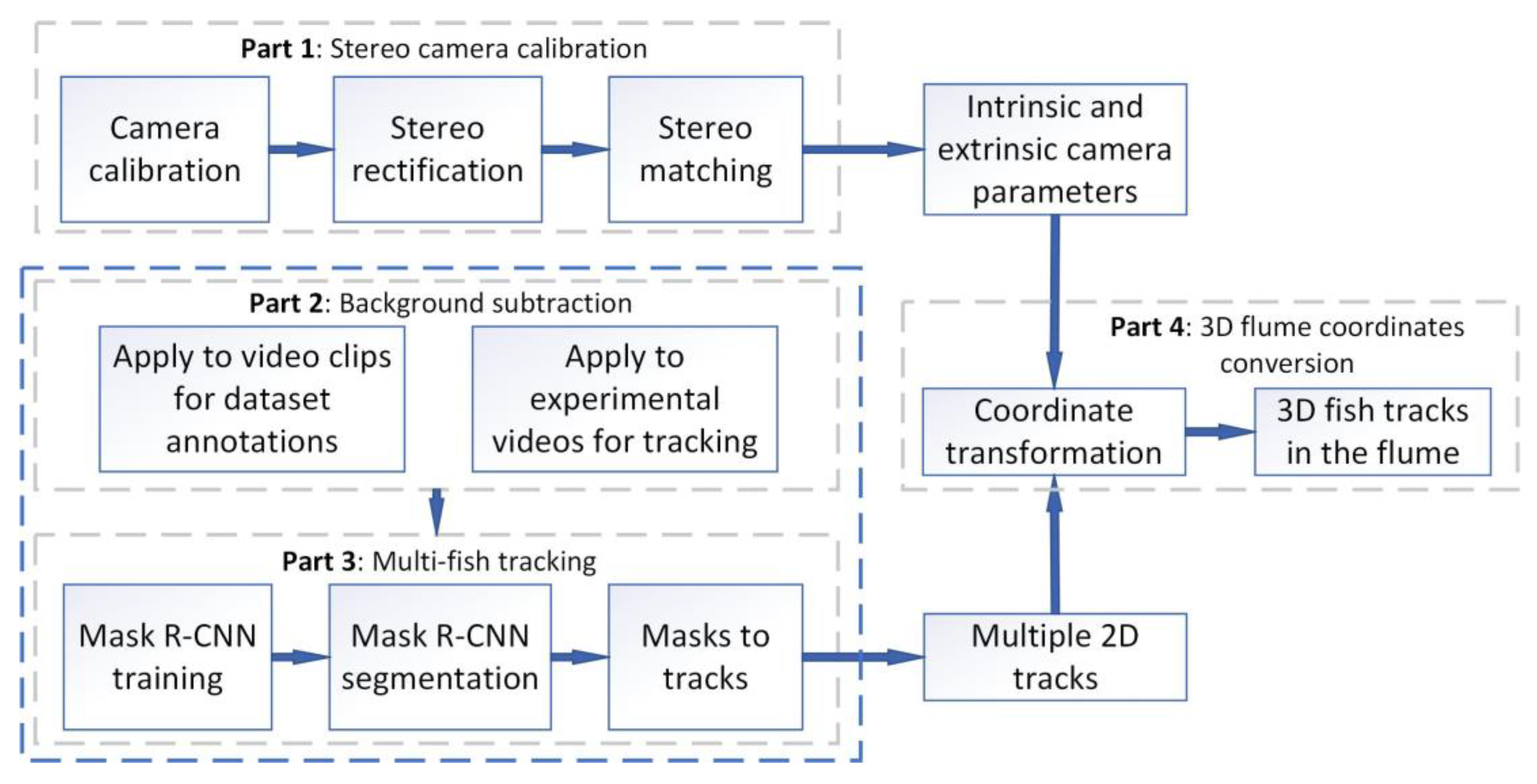
With Mask R-CNN as the tracking core, this study reports an improved, well-documented, and open-source 3D fish tracking system (FishSeg) to deal with 3D fish tracking in large etho-hydraulic flumes with multiple fisheye cameras. FishSeg consists of four parts: (1) stereo camera calibration, (2) background subtraction, (3) multi-fish tracking (the core of FishSeg), and (4) 3D flume coordinates conversion. Compared to [19], the “Camera Calibration” part remains unchanged. “Background Subtraction” and “Multi-fish Tracking” were improved, while the “3D Conversion” was adapted based on the new 2D tracking results. The source code of FishSeg and its guidelines can be found in [31].

2. Fish Videos

To mitigate the negative effects of hydropower plants on fish passage, VAW of ETH Zurich has conducted research on downstream fish protection and guidance racks for more than 10 years with various fish species, including barbel (Barbus barbus), spirlin (Alburnoides bipunctatus), nase (Chondrostoma nasus), European eel (Anguilla anguilla), brown trout (Salmo trutta), chub (Squalius cephalus) and salmon (Salmo salar). Video recordings of the live fish tests performed in [2,4] were selected and used in this study. The detailed setup and procedure of the live fish tests have been described in [2,4], while only the characteristics relevant to the video tracking are described here. The setup consisted of a 30 m long, 1.5 m wide, and 1.4 m deep flume with a water depth of 0.9 m (Figure 1). Six halogen lamps (1000 W) were positioned on the right flume side directed at a white linen sheet hanging over the flume for uniform illumination. Five top-view cameras were placed at a distance of 1.3 m to 1.5 m from each other to ensure sufficient overlaps of the field of view (Figure 1a). The section of the flume covered by the cameras had a length of up to 8 m and a width of 1.5 m. The waterproof casing of the cameras was submerged by 5 cm to reduce air entrainment and bubbles. Each camera of type acA2040-35gm (Basler) with a maximal resolution of 2048 × 1536 px2 was equipped with a 185° fisheye lens of type FE185C086HA-1 (Fujifilm) and waterproofed with IP67-enclosures Orca S (autoVimation) (Figure 1b). The cameras were set to record 20 frames per second.
During experiments, three fish of the same species were placed in the flume at a time, which needed to be distinguished by the tracking code. Of the tested fish species, trout, spirlin, barbel, salmon, chub, and nase have similar body shapes and color contrast to the flume bottom and are, therefore, very similar from the point of view of a fish tracking algorithm. Eels are much larger in length and have different body shapes, i.e., slender and elongated. Brown trout were chosen as representative of the classical “fish shape”, while European eels need a differently trained dataset. Both were used to evaluate the difference between the tracking code of [19] and FishSeg. The total lengths (TL) of the tested trout and eel were 11.57 ± 2.71 cm and 71.73 ± 4.32 cm, respectively.

3. 3D Fish Tracking

The workflow indicating how the four parts of FishSeg interact with each other is illustrated in Figure 2. The detailed development process of the four parts is described in the following subsections.

3.1. Stereo Camera Calibration

The fisheye cameras were calibrated following the procedure described in [19] on a set of videos with a checkerboard moving slowly through the entire volume of the flume. Generally, the calibration contained three main steps: (1) finding the intrinsic parameters for each fisheye-distorted camera, (2) calibrating the intrinsic and local extrinsic parameters of the stereo camera system based on the overlapping views of camera pairs, and (3) performing a rigid transformation of all camera pairs to the global flume coordinate system.
To be more specific, for step (1), image frames with a checkerboard (square sizes of 39.9 mm) at different angles and distances were automatically preselected from the calibration video series. The crossing points on the checkerboard were detected from the preselected video frames with the checkerboard edges enhanced with fast local Laplacian filters. In the meantime, the preselected video frames were undistorted by applying the fisheye-lens model of [32]. In the next step, a standard frame camera model from Matlab (https://ww2.mathworks.cn/help/vision/camera-calibration.html (accesssed on 23 August 2023)) was applied to the undistorted frames to estimate the intrinsic and extrinsic parameters for the stereo calibration. Finally, with 43 fixed reference points at the flume bottom, the point coordinates were manually digitized on the static images from camera pairs. Based on the point pairs, each camera coordinate system was shifted and rotated by a rigid transformation to a global flume coordinate system. As a result, fish tracks in pixel coordinates on distorted video frames can be converted to Cartesian real-world coordinates.

3.2. Background Subtraction

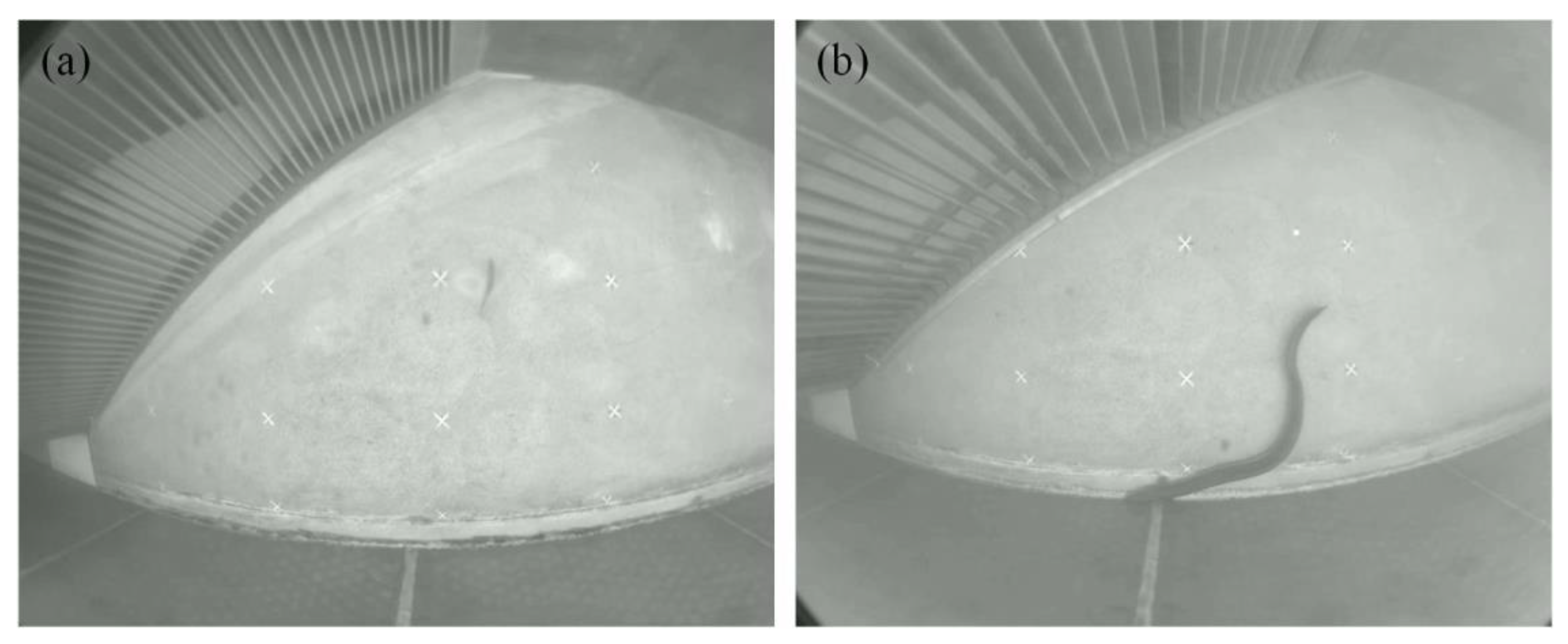
Two main problems that affected the tracking quality of Detert’s code were the detection of low-color-contrast fish and the interference of fish shadows [19]. To present an impression of our video quality, two frames collected from the experimental videos for trout and eel tests are displayed in Figure 3. For such videos, Ref. [19] computed the median background from 100 frames equally selected from the entire video sequence and converted each filtered image into a binary image. By comparison between the tracked image and the background image at an absolute difference of <8-pixel intensities, the moving objects could be separated from the background image. However, the subtraction results were not satisfying due to two reasons [19]. Firstly, the body color and size of fish could change when fish swam around at different vertical depths. Secondly, the illumination conditions changed rapidly with surges of air bubbles or light reflections. Thus, the traditional background subtraction method with a fixed threshold for pixel intensities could not meet the requirements under such complicated experimental conditions.
After a review of the state-of-the-art background subtraction methods, BackgroundSubtractorMOG2 from the OpenCV Library was selected, which was easy to use and suitable for the present case. The MOG2 is a Gaussian Mixture-based Background/Foreground Segmentation Algorithm [33,34]. Compared to the former algorithm MOG, MOG2 has an added feature of selecting the appropriate number of Gaussian distributions for each pixel rather than taking a K Gaussian distribution throughout the algorithm. Thus, this feature provides better adaptability to scenes with illumination changes and object shadows, which are useful for the present study.
By implementing the MOG2, each frame from the experimental video was first converted into a binary image with foreground masks in a new “pre-processed” video rather than directly fed into the tracking algorithm as the traditional subtraction does. Note that the size of the pre-processed video was much smaller than the original video, and the converting process was faster. Two additional functions were added to the new background subtraction method. First, the start time could be specified to start tracking only at the timestep in the video when fish were present, which was manually noted during the experiments. Second, the frequency of frame selection could be set to reduce the pre-processed frames. For instance, if the frequency was set as 5, the algorithm only processed one frame from every five frames. This function is useful if long videos or short videos with a high frame rate are treated with no high requirements for tracking accuracy. Both functions reduce the tracking time in the next step.

3.3. Automated Fish Detection and Tracking

3.3.1. FishSeg Architecture

Compared to the previously developed tracking code by [19], automated fish segmentation and tracking are the major improved parts of FishSeg, which are based on the Mask R-CNN architecture (see Figure 4). The architecture contains a two-stage framework: the first stage scans the image and generates proposals (areas likely to contain an object); the second stage classifies the proposals and generates bounding boxes and masks. Herein, the ResNet101 and the Feature Pyramid Network (FPN) as the basis of convolutional backbone architecture are implemented. A brief description of each following step is given below:
  • The frame is passed through a convolutional network;
  • The output of the first Conv Nets is fed to the Region Proposal Network (RPN), which creates different anchor boxes (Regions Of Interest, ROI) for any detected objects;
  • The anchor boxes are passed through to the ROI Align stage, which converts ROIs into the same size required for further processing;
  • The outputs of the normalized ROIs are sent to fully connected layers, which classify the object in the specific region and locate the position of the bounding box;
  • The outputs from the ROI Align stage are parallelly sent to Conv Nets in order to generate a mask of the object pixels.
The network is trained using Stochastic Gradient Descent (SGD) to minimize a multi-task loss of each ROI (see Equation (1)):
L = Lrpn-class + Lrpn-bbox + Lmrcnn-class + Lmrcnn-bbox + Lmrcnn-mask
where L is the total loss of the network, Lrpn-class is the loss assigned to improper classification of anchor boxes by RPN, Lrpn-bbox corresponds to the localization accuracy of the RPN, Lmrcnn-class is the loss assigned to improper classification of objects present in the region proposal, Lmrcnn-bbox is the loss assigned on the localization of the bounding box of the identified class, and Lmrcnn-mask denotes masks created on the identified objects. Note that the learning curves of each loss can be used to diagnose the model performance.
Intersection over Union (IoU) and mean Average Precision (mAP) are widely used metrics used to evaluate the object detection performance of Mask R-CNN models. IoU is defined as the area where the prediction overlaps with the ground box (Intersection) divided by the total area covered by both the prediction and ground box (Union). An IoU score larger than 0.5 indicates that more than half of the predicted box overlaps with the ground box. In Mask R-CNN, the default IoU threshold is set as 0.5 to determine good mask predictions [35]. In contrast, the mean Average Precision (mAP) is defined by the relationship between Precision (P) and Recall (R), which quantifies the model performance of obtaining the right segmentation masks [36]. Precision is the proportion of correctly predicted targets in the positive class (scores above the IoU threshold), while Recall is the proportion of correctly predicted targets in all predicted targets. Values of P, R, and mAP can be calculated from Equations (2)–(4):
P r e c i s i o n P = T r u e P o s i t i v e ( T P ) T r u e P o s i t i v e T P + F a l s e P o s i t i v e ( F P )
R e c a l l R = T r u e P o s i t i v e ( T P ) T r u e P o s i t i v e T P + F a l s e N e g a t i v e ( F N )
m A P = 0 1 P ( R ) d R
In practice, a correctly predicted target (True Positive—TP) is obtained only when the IoU is scored above 0.5. The mAP score is generally calculated as the mean of the Average Precision (AP) scores among all images evaluated.

3.3.2. Application of FishSeg in Fish Tracking

Both training and validation datasets used in this study were annotated from fisheye-distorted video clips where the target fish were present in the camera shooting range. All videos had a resolution of 2048 × 1536 px2 and a frame rate of 20 fps. The Python package TrackUtil, developed by [37], was applied to make annotations for videos. TrackUtil also supported the simultaneous play of multiple videos, which was quite useful for making datasets from stereo video streams. Annotations were stored in HDF5 format, which allowed for flexible data storage of both annotation metrics and annotated images. In addition, the annotated images could undergo image augmentation, including horizontal and vertical flips, as well as changes in image brightness, contrast, saturation, and hue. The pre-trained weight trained on the MS COCO dataset [38] was used as the initial weight, and thus, transfer learning could be performed with small datasets for good mask predictions.
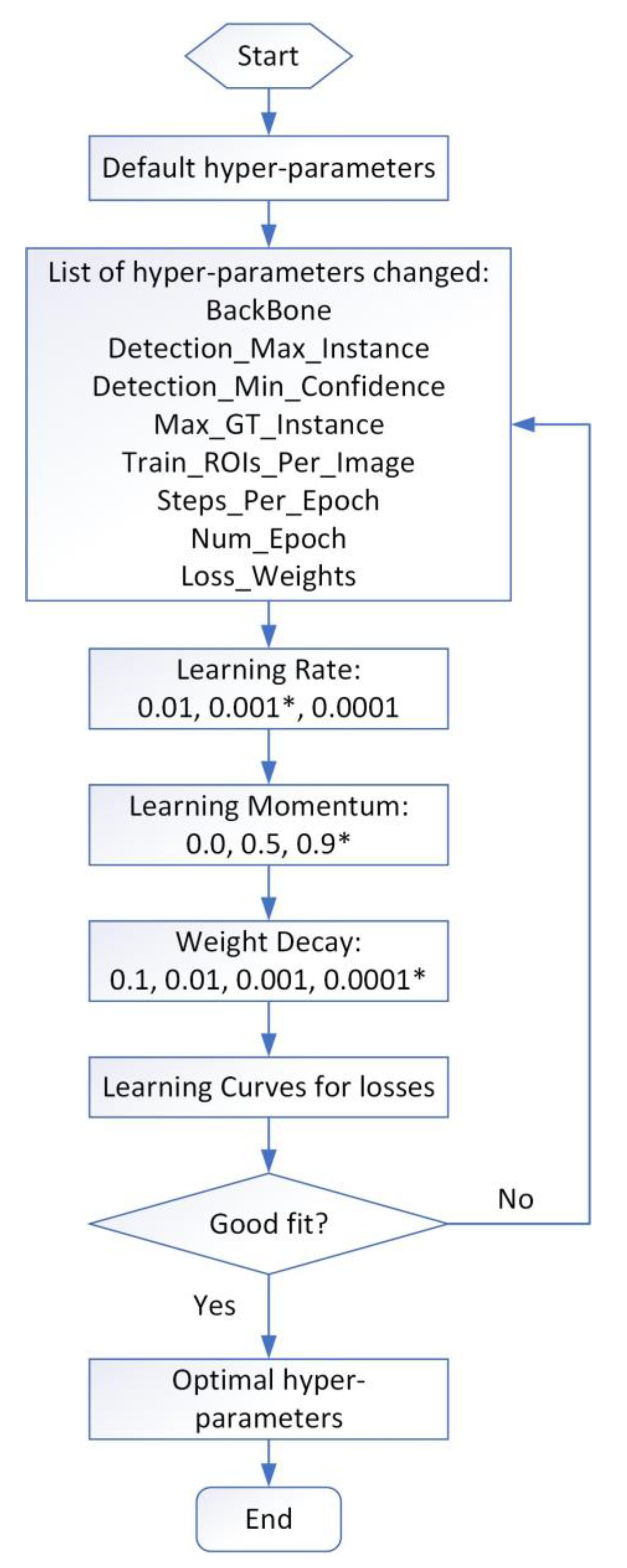
After loading the datasets into the model, the hyper-parameters were fine-tuned for stable model performance. The process of finding the optimal hyper-parameters is displayed in Figure 5, which includes the hyper-parameters specific to FishSeg, such as Train_ROIs_Per_image, Max_GT_Instances, and Detection_Min_Confidence. All the hyper-parameters are important for the training speed and accuracy of the model, with the learning rate, learning momentum, and weight decay being crucial for model performance since they determine whether the optimal solution is found or not. The environment information for the model training is provided in Table S1.
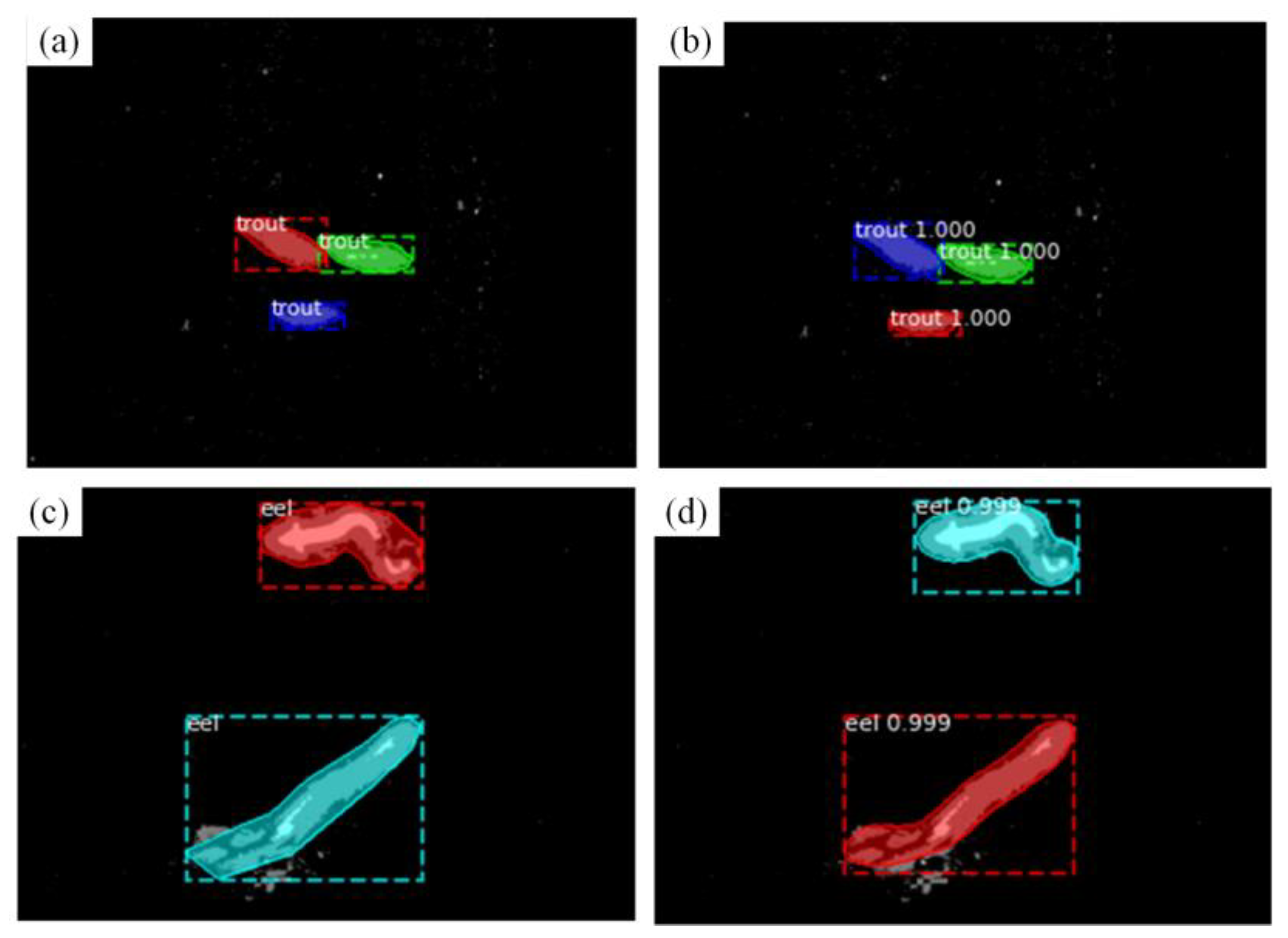
The number of images and annotations included in each dataset for trout and eel models is listed in Table 1, with two annotated image samples for trout and eel displayed in Figure 6a,c, respectively. To ensure the validity of image samples, the number of fish in each image was 1, 2, or 3 since only three fish were released from the starting compartment for each test.
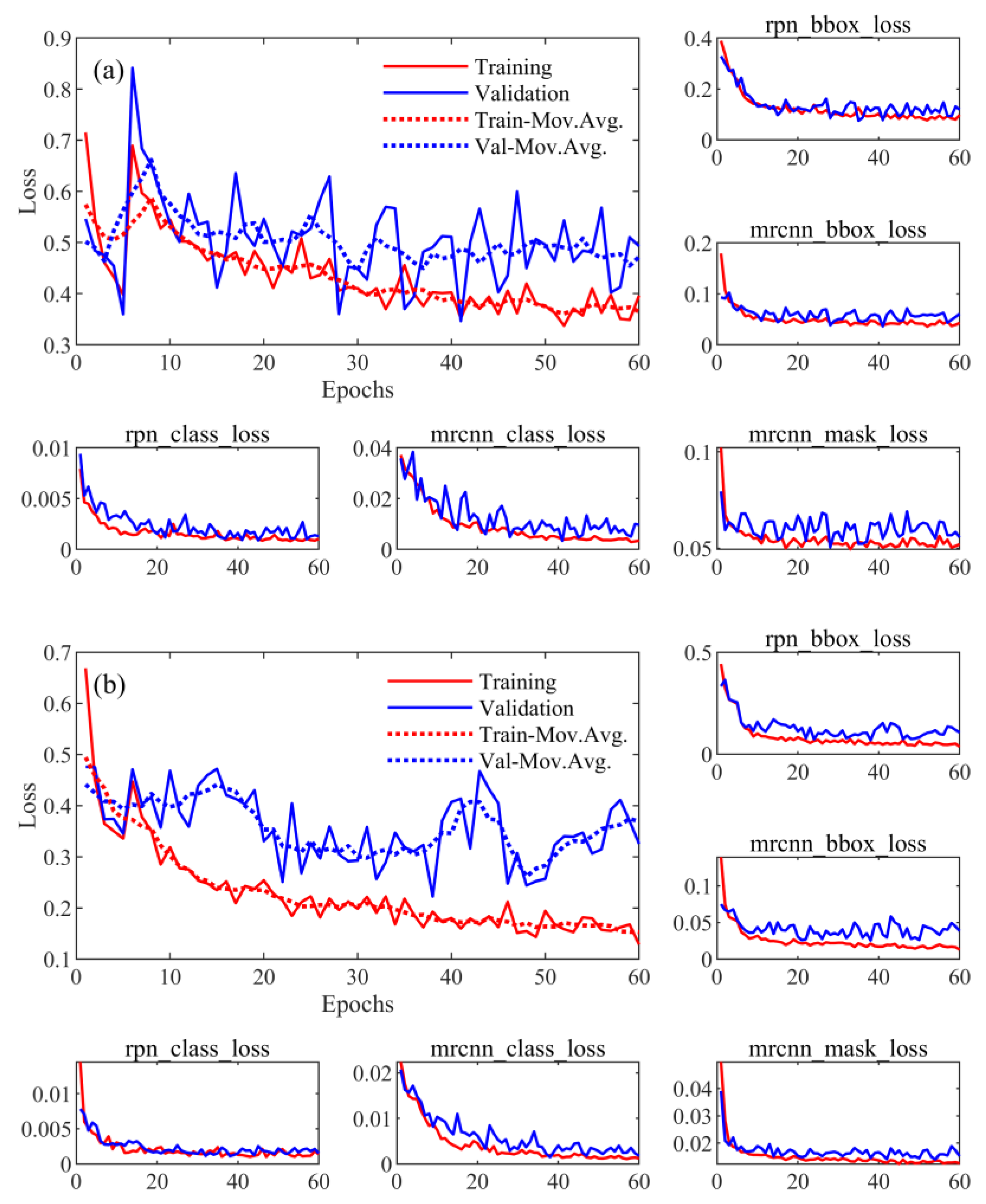
For each combination of hyper-parameter setups, the model performance can be compared in three ways. First, evaluation through mAP for validation datasets, which were 0.837 and 0.876 for trout and eel models, respectively, in the present study. The second way is to check the training results by visualizing the performance on part of the validation dataset. For instance, visualizations of validation images are shown in Figure 6, with Figure 6a,b for trout images and Figure 6c,d for eel images. For each set of images, the left image is annotated from pre-processed video clips, while the right one is from the mask prediction made using FishSeg. Each prediction is marked with a score ranging from 0 to 1, with 1 denoting the best prediction result. Finally, the model performance is evaluated from training and validation losses automatically generated in the log file. The training curve gives an idea of how well the model is learning, while the validation curve indicates how well the model is generalizing. Good-fit learning curves can be identified from two features. On the one hand, both training and validation losses decrease to a point of stability. In addition, the validation curve has a small gap with the training curve. In this study, a 5-point moving average was used to smooth both learning curves for clearer trends. Following the above rules for diagnosing the model performance, the final fine-tuned hyper-parameters for the improved FishSeg model for trout and eel are listed in Table S2, in contrast with the default setups in Mask R-CNN. Note that the loss weights of mrcnn_bbox_class and mrcnn_mask_loss were reduced for both trout and eel models since precise localization (denoted by mrcnn_bbox_class) and identification of target fish at the pixel level (denoted by mrcnn_mask_loss) were not the top priorities for fish tracking in FishSeg. With the optimal hyper-parameter setup listed in Table S2, learning curves for trout and eel models are shown in Figure 7. Large fluctuations in the total loss (top left) were common for mini-batch training data and did not indicate an overfit to a small dataset. Furthermore, trends of the five sub-losses for both models followed the two criteria diagnosing good-fit curves, which proved that both trout and eel models achieved good performances in a relatively short time (both at 60 epochs).
After the training process was completed, the FishSeg model was saved and directly applied to the fish tracking process. During the tracking process, the model conducted mask predictions for every frame of the pre-processed videos and saved them into HDF5 format files. Further work was required to convert masks to tracks and associate individual tracks across frames.

3.3.3. Converting Masks to Tracks

Based on the works of [37], the “mask2tracks” script was implemented in the “Multi-fish Tracking” part of the FishSeg workflow to convert the mask predictions into tracks of multiple fish. The script consisted of three main functions, which were centroid calculation, track assignment, and batch processing support. During the conversion process, the centroids of mask predictions were first calculated from mask location metrics. Then, the Euclidean distances among fish centroids were calculated and fed into the function of “linear_sum_assignment”, which returned the optimal assignment of fish identities based on a modified Jonker-Volgenant algorithm with no initialization [39]. Thus, individual tracks per frame could be converted into track sequences, with each sequence being assigned a unique identity.

3.4. Conversion into 3D Flume Coordinates

The basic principle of converting 2D tracks from overlapping camera views to 3D flume coordinates in FishSeg is the same as that of [19]. First, tracks in each camera were undistorted using the intrinsic and extrinsic camera parameters obtained from the calibration procedure. Second, the assignment of synchronous track pairs from overlapping camera views was conducted with the nearest-neighbor criterion [40]. Finally, the epipolar geometry for each camera was applied to synchronous tracks, which transferred the 2D tracks into a 3D metric space [41]. Instead of undistorting each image frame before the tracking, 2D tracks were found first, followed by the calibration procedure to optimize the computation time.
Following the same principle, two major improvements were made in the 3D conversion part of FishSeg for better performance. Specifically, with the fish tracks obtained from FishSeg, the redundant part dealing with misidentifications from the original code was removed, which reduced the processing time for 3D conversion. In addition, FishSeg can delete very short tracks, which were usually misidentifications caused by air bubbles or light reflections. The threshold to determine the misidentified short tracks can be adjusted manually based on the actual tracking results.

4. Results

Both the tracking codes of [19] and FishSeg were applied to obtain 3D tracks for the selected trout and eel experiments. To reduce tracking time for FishSeg, the frequency for frame selection was set to 2, which meant the lengths of processed videos were only half as long as that of the original video.
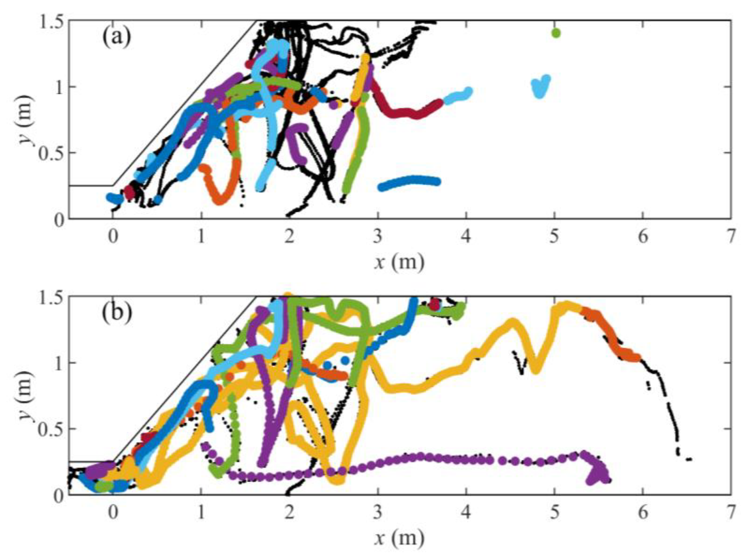
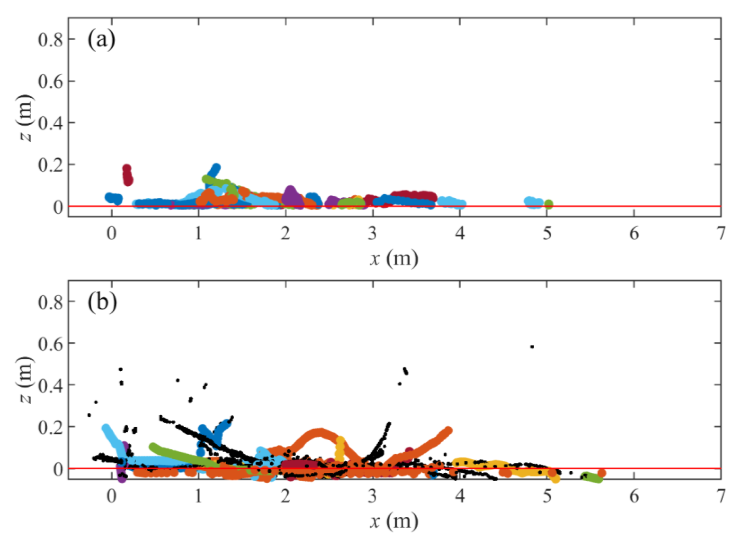
The top view of trout tracks is presented in Figure 8, with black dots separately tracked from five cameras and colored dots indicating the merged fish tracks. As displayed in Figure 8, trout tended to swim interactively, especially near the fish guidance rack and bypass, which could lead to misidentification of fish IDs with overlapping or occlusions. A comparison of Figure 8a,b shows that trout tracks obtained from FishSeg were more connected and continuous compared to those obtained with Detert’s code [19]. Specifically, in Figure 8a, tracks from x = 4 m to x = 6.5 m are highly discontinuous, indicating that fish were not tracked at all or filtered out in this range. This could result from the low color contrast between fish and flume bottom or the relatively small body size of fish. In addition, when three trout swam close to each other near the rack, occlusions could happen with overlapping mask predictions. Thus, their tracks were identified as separate individuals, leading to excessive unconnected tracks. However, some of the lost track points between x = 4 m and x = 6.5 m in Figure 8a were found successfully by FishSeg, and the tracks were more continuous near the rack area where strong fish interactions were observed (Figure 8b). Side-views of trout tracks are also presented in Figure 9 as a supplementary illustration of 3D fish tracks. In Figure 9a, almost all trout tracks were vertically distributed within the range of z = 0~0.1 m, while in Figure 9b, FishSeg could successfully track trout that swam up to z = 0.2 m. This again proved the advancement of FishSeg tracking for trout swimming close to the flume bottom.
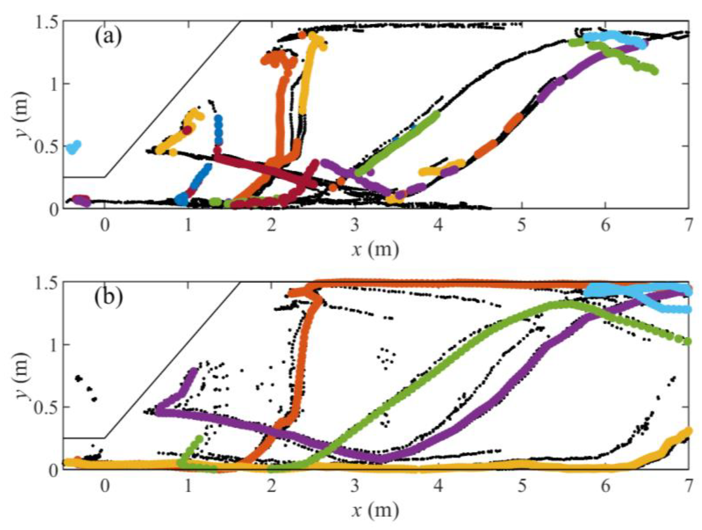
Similarly, the top views of eel tracks from Detert’s code [19] and FishSeg are presented in Figure 10. Compared to trout tracks in Figure 8, eel tracks in Figure 10 are more uniformly distributed along the whole flume and less interactive, indicating that eels were easier to track than trout in the same experiment setup. Figure 10b displays less segmented eel tracks throughout the flume than those in Figure 10a. In addition, FishSeg could obtain eel tracks that were barely tracked using Detert’s code [19], such as the yellow tracks close to the right flume wall at x = −0.5~7 m, the green tracks at x = 4~6 m, and orange tracks close to the left flume wall at x = 2.5~6.5 m. Moreover, side-view eel tracks in Figure 11 illustrate that eels tended to swim near the flume bottom just as trout did but more actively. Comparison between Figure 11a,b indicates that FishSeg again presented better tracking performance at the vertical plane, especially for the ranges of x = −0.5~1.5 m and x = 4~7 m. Comparison of 3D tracks between trout (Figure 8b and Figure 9b) and eel (Figure 10b and Figure 11b) shows that FishSeg presents a higher level of continuity and accuracy in tracking eel since eel were easier to be recognized due to their larger body size, characteristic body shape, and less interactive swimming pattern.
To quantitatively compare the tracking performance of FishSeg and Detert’s code, tracking parameters, including the frame selection frequencies (freq), total lengths of tracks (lg), and the number of segmented tracks (num) are summarized in Table 2 for both trout and eel. In Table 2, freq = 1 means every frame is tracked for Detert’s code, while for FishSeg, only every second frame is analyzed (freq = 2). The continuity of each track set is calculated using freq×g/num, which measures the average length of each segmented track. The continuity ratio (CR) is thus proposed to compare the tracking quality of FishSeg against that of Detert’s code, see Equation (5):
C R = f r e q 1 × l g 1 / n u m 1 f r e q 2 × l g 2 / n u m 2
with subscript 1 denoting tracking parameters related to FishSeg and subscript 2 indicating parameters in fish tracking using Detert’s code.
As listed in Table 2, the number of segmented tracks obtained using Detert’s code is approximately 4 and 5 times higher than that by FishSeg for trout and eel, respectively. CR values further indicate that the continuity of tracks obtained using FishSeg is about three times higher than that by Detert’s code, noting that the CR value for eel is slightly higher than that for trout.

5. Discussion

5.1. Improvements and Limitations of FishSeg

Based on the work of [19], an improved 3D fish tracking code (FishSeg) using a modified Mask R-CNN model was developed to provide clearer information on fish behavior in large experimental flumes. From the qualitative comparison of tracks in Figure 8, Figure 9, Figure 10 and Figure 11, FishSeg greatly improved the accuracy in multiple fish tracking, while the quantification of tracks in Table 2 illustrates that the continuity of tracks by FishSeg was at least three times higher than Detert’s code [19]. Despite the improvements in tracking results, the application of FishSeg is still limited in several aspects, such as tracking speed, segmented tracks, species classification, and pose estimation. The key problem that affected the use of FishSeg was the tracking speed. In Detert’s code, a Kalman filter was used to predict the object’s future locations. In contrast, in the FishSeg, every frame fed into the model was considered an independent image, and the model needed to make independent predictions for possible masks, not just locations, for each image. Thus, for a 30-minute experimental video, it took 30–40 min to finish tracking with the original tracking code, while 2 h was needed using FishSeg (with two images per GPU). To fix this problem, the function of frame selection frequency was developed in the “Background Subtraction” part, which could reduce the tracking time to 1 h if the frequency is set to 2, and less if the frequency is higher. In addition, if a computer with high-performance GPUs (such as NVIDIA RTX A5000 with 24 GB memory used in this study, NVIDIA, Santa Clara, CA, USA) is available, the tracking can be conducted simultaneously with multiple processes, which can make the tracking time acceptable.
As shown in Table 2, the number of segmented tracks generated by FishSeg was more than the actual number of fish tested in the live-fish tests (n = 3) for both trout (num = 26, Figure 8b) and eel (num = 5, Figure 10b). One possible reason for the excessive segmented tracks was that fish could be assigned a different ID each time they re-entered the observation area. Another reason was that FishSeg could lose fish tracks for a short time when fish could not be recognized, or occlusion happened with overlapping fish. The first reason accounts for the two additional track series in the eel example, while the second one explains the excessive track series in the trout example. Despite such limitations in segmented tracks, FishSeg still has the potential to identify preferred hydraulic regions of fish through heatmaps or sector analysis [2,4]. Nevertheless, with more continuous tracks, it would be easier to calculate the swimming speed or acceleration of fish through fish tracks without further manual post-process of segmented tracks.
As mentioned above, FishSeg analyses needed more time on track due to the function of mask predictions, which is both the weakness and strength of Mask R-CNN. FishSeg, with the function of mask predictions, possessed the potential to make species classification and pose estimation of fish (i.e., direct evaluation of rheotaxis changes) [30]. Species classification and tracking were possible with the FishSeg model since it identified individuals by learning the characteristics of their body shape and size. However, in this study, the selected comparison cases were aimed at trout or eel groups without a mixture; therefore, no species identification was conducted. In contrast, tracking various fish species was not possible with Detert’s code since the threshold for object detection was set to a fixed size based on the expected object size. Therefore, if trout and eel were tested together in one flume, a threshold that enabled the recognition of trout and eel (a very large size range) could cause misidentifications for any disturbance whose pixel area was within the threshold range. This problem can be easily solved using the FishSeg model since trout and eel have completely different body shapes.
In this study, factors that affected the tracking quality of fish included low color contrasts between fish and the flume bottom, as well as fish shadows on the flume bottom. To deal with such disturbances, BackgroundSubtractorMOG2 was applied, which turned both fish and fish shadow into the foreground mask. Nevertheless, considering fish with its shadow could deform or blur the original body shape of fish, which caused relatively large deviations if pose estimations were applied. In general, for live-fish experiments, the setup should aim at creating high color contrasts between the fish and its background, while uniform illumination from all sides should also be applied to reduce the interference of shadows as much as possible.

5.2. Comparison with Other R-CNN-Based Models

The Mask R-CNN applied here was the newest branch of the R-CNN family, which has revolutionized the object detection area in computer vision during the last few years. The advancement of Mask R-CNN was assessed and compared using mAP values.
Before the announcement of Mask R-CNN, its predecessors, Fast R-CNN and Faster R-CNN, had already shown better performance in object detection than other algorithms, such as SPP-Net, with much less training and test time, and thus have been used in works about fish behavior [21]. The performance metrics of different R-CNN-based models are presented in Table 3, with the mAP values as the main indicator. Specifically, the modified Fast R-CNN in the work of [25] achieved an average mAP accuracy of 0.814 over 12 fish species. Ref. [27] trained Faster R-CNN on a dataset of 4909 images (12,365 annotations) of 50 fish species. With the application of transfer learning, they found that Faster R-CNN presented a comparable mAP accuracy of 0.824 with further reduced training and test time relative to the previous state-of-the-art Fast R-CNN method.
With the additional function of predicting a segmentation mask on the target object, the current state-of-the-art Mask R-CNN was transferable to deal with object detection problems for fish tracked in underwater videos. For instance, Ref. [24] fed a dataset of 6080 annotations into pre-trained Mask R-CNN, which achieved a mAP accuracy of 0.925 on the test set and 0.934 on naval footage collected from a different location. Moreover, Ref. [30] trained the Mask R-CNN on the Roman seabream dataset of 2015 images (2541 annotations). With an IoU threshold of 0.5, the Roman seabream model achieved a mAP of 0.803 and 0.815 on the validation and test set, respectively. The FishSeg model in this study achieves a mAP of 0.837 and 0.876 for the validation datasets of trout and eel, respectively. Although lower than the mAP of [24], the mAP of the FishSeg model still shows that it presents good tracking performance with smaller datasets (see Table 1) since it is quite close to 1.0. Furthermore, under the same IoU threshold, the mAP of the FishSeg model was higher than that of the seabream model, with fewer annotations and training time [30].

6. Conclusions

The present study improved a previously developed fish-tracking system [19] by replacing the fish-tracking algorithm with a combination of BackgroundSubtractorMOG2 and modified Mask R-CNN, as well as adapting the 3D conversion part. The newly developed workflow is referred to as “FishSeg”. Brown trout and eel were selected as target species to evaluate how FishSeg performed for fish of different sizes and body shapes. The comparison of fish tracks indicated that FishSeg presented better accuracy for tracking both trout and eel than the original tracking code. Moreover, the values of tracking continuity ratio were more than 3 for trout and eel tracks, which showed that FishSeg was more advantageous over Detert code in getting continuous tracks. Comparison with other R-CNN-based models further confirmed the tracking accuracy of the FishSeg model with a mAP of 0.837 and 0.876 for trout and eel, respectively.
FishSeg thus provides a robust way to generate fish tracks in large experimental flumes and enables further behavioral analysis, i.e., heat maps and analysis of swimming speed. Further improvements to the tracking accuracy can be achieved by providing homogenous illumination and improving the color contrast between the flume background and the fish. Unfortunately, this is often not possible as a nature-like color of the background is desirable. The present results will underpin more research studies on 3D fish tracking and contribute to the research on the fish behavior and development of fish passage structures in laboratory conditions.

Supplementary Materials

The following supporting information can be downloaded at: https://www.mdpi.com/article/10.3390/w15173107/s1, Table S1: Experimental environment information to implement the FishSeg model; Table S2: Hyper-parameter setups for the default Mask R-CNN model and the improved FishSeg model for trout and eel. Note that hyper-parameters for the default Mask R-CNN model are aimed at the shapes example provided by the Matterport team.

Author Contributions

Conceptualization, F.Y., A.M.-R. and I.A.; Methodology, F.Y.; Software, F.Y.; Validation, F.Y., Writing—Original Draft, F.Y., Visualization, F.Y., A.M.-R. and I.A.; Writing—Review and Editing, A.M.-R., R.M.B., Y.Z. and I.A.; Supervision, R.M.B., Y.Z. and I.A.; funding acquisition, Y.Z. All authors have read and agreed to the published version of the manuscript.

Funding

This work is financially supported by the China Scholarship Council (No. 202106240067) and conducted at VAW of ETH Zurich.

Data Availability Statement

Not applicable.

Acknowledgments

The authors are grateful to Peijun Li for offering great help in implementing the Mask R-CNN model for fish tracking and improving the model performance. The authors are also thankful for Robert Mario Naudascher, who provides valuable suggestions in implementing the BackgroundSubtraction part in our code.

Conflicts of Interest

The authors declare no conflict of interest.

References

  1. Albayrak, I.; Boes, R.M.; Kriewitz, C.R.; Peter, A.; Tullis, B.P. Fish guidance structures: Hydraulic performance and fish guidance efficiencies. J. Ecohydraulics 2020, 5, 113–131. [Google Scholar] [CrossRef]
  2. Beck, C.; Albayrak, I.; Meister, J.; Peter, A.; Boes, R.M. Swimming Behavior of Downstream Moving Fish at Innovative Curved-Bar Rack Bypass Systems for Fish Protection at Water Intakes. Water 2020, 12, 3244. [Google Scholar] [CrossRef]
  3. Silva, A.T.; Lucas, M.C.; Castro-Santos, T.; Katapodis, C.; Baumgartner, L.J.; Thiem, J.D.; Aarestrup, K.; Pompeu, P.S.; O’brien, G.C.; Braun, D.C.; et al. The future of fish passage science, engineering, and practice. Fish Fish. 2018, 19, 340–362. [Google Scholar] [CrossRef]
  4. Meister, J.; Selz, O.M.; Beck, C.; Peter, A.; Albayrak, I.; Boes, R.M. Protection and guidance of downstream moving fish with horizontal bar rack bypass systems. Ecol. Eng. 2022, 178, 106584. [Google Scholar] [CrossRef] [PubMed]
  5. Lehmann, B.; Bensing, K.; Adam, B.; Schwevers, U.; Tuhtan, J.A. Ethohydraulics: A Method for Nature-Compatible Hydraulic Engineering; Springer Nature: New York, NY, USA, 2022. [Google Scholar]
  6. Noldus, L.P.J.J.; Spink, A.J.; Tegelenbosch, R.A.J. EthoVision: A versatile video tracking system for automation of behavioral experiments. Behav. Res. Methods Instrum. Comput. 2001, 33, 398–414. [Google Scholar] [CrossRef] [PubMed]
  7. Roth, M.S.; Wagner, F.; Tom, R.; Stamm, J. Ethohydraulic Laboratory Experiments on Fish Descent in Accelerated Flows. Wasserwirtschaft 2022, 112, 31–37. [Google Scholar]
  8. Graving, J.M.; Chae, D.; Naik, H.; Li, L.; Couzin, I.D. DeepPoseKit, a software toolkit for fast and robust animal pose estimation using deep learning. elife 2019, 8, e47994. [Google Scholar] [CrossRef]
  9. Mathis, A.; Mamidanna, P.; Cury, K.M.; Abe, T.; Murthy, V.N.; Mathis, M.W.; Bethge, M. DeepLabCut: Markerless pose estimation of user-defined body parts with deep learning. Nat. Neurosci. 2018, 21, 1281–1289. [Google Scholar] [CrossRef]
  10. Pereira, T.D.; Aldarondo, D.E.; Willmore, L.; Kislin, M.; Wang, S.S.; Murthy, M.; Shaevitz, J.W. Fast animal pose estimation using deep neural networks. Nat. Methods 2019, 16, 117–125. [Google Scholar] [CrossRef]
  11. Pereira, T.D.; Tabris, N.; Li, J.; Ravindranath, S.; Murthy, M. SLEAP: Multi-Animal Pose Tracking; Cold Spring Harbor Laboratory: New York, NY, USA, 2020. [Google Scholar]
  12. Romero-Ferrero, F.; Bergomi, M.G.; Hinz, R.C.; Heras, F.J.; De Polavieja, G.G. Idtracker. ai: Tracking all individuals in small or large collectives of unmarked animals. Nat. Methods 2019, 16, 179–182. [Google Scholar] [CrossRef]
  13. Walter, T.; Couzin, I.D. TRex, a fast multi-animal tracking system with markerless identification, and 2D estimation of posture and visual fields. eLife Sci. 2021, 10, e64000. [Google Scholar] [CrossRef] [PubMed]
  14. Rodriguez, Á.; Bermúdez, M.; Rabuñal, J.R.; Puertas, J.; Dorado, J.; Pena, L.; Balairón, L. Optical fish trajectory measurement in fishways through computer vision and artificial neural networks. J. Comput. Civ. Eng. 2011, 25, 291–301. [Google Scholar] [CrossRef]
  15. Hedrick, T.L. Software techniques for two- and three-dimensional kinematic measurements of biological and biomimetic systems. Bioinspiration Biomim. 2008, 3, 34001. [Google Scholar] [CrossRef] [PubMed]
  16. Butail, S.; Paley, D.A. Three-dimensional reconstruction of the fast-start swimming kinematics of densely schooling fish. J. R. Soc. Interface 2012, 9, 77–88. [Google Scholar] [CrossRef] [PubMed]
  17. Neuswanger, J.R.; Wipfli, M.S.; Rosenberger, A.E.; Hughes, N.F. Measuring fish and their physical habitats: Versatile 2D and 3D video techniques with user-friendly software. Can. J. Fish. Aquat. Sci. 2016, 73, 1861–1873. [Google Scholar] [CrossRef]
  18. Detert, M.; Schütz, C.; Czerny, R. Development and tests of a 3D fish-tracking videometry system for an experimental flume. In Proceedings of the 9th International Conference on Fluvial Hydraulics, Lyon-Villeurbanne, France, 5–8 September 2018. [Google Scholar]
  19. Detert, M.; Albayrak, I.; Boes, R.M. A New System for 3D Fish-Tracking; FIThydro Report; Laboratory of Hydraulics, Hydrology and Glaciology (ETH): Zurich, Switzerland, 2019. [Google Scholar] [CrossRef]
  20. Meister, J.; Moldenhauer-Roth, A.; Beck, C.; Selz, O.M.; Peter, A.; Albayrak, I.; Boes, R.M. Protection and Guidance of Downstream Moving Fish with Electrified Horizontal Bar Rack Bypass Systems. Water 2021, 13, 2786. [Google Scholar] [CrossRef]
  21. He, K.; Zhang, X.; Ren, S.; Sun, J. Spatial pyramid pooling in deep convolutional networks for visual recognition. IEEE Trans. Pattern Anal. Mach. Intell. 2015, 37, 1904–1916. [Google Scholar] [CrossRef]
  22. Alshdaifat, N.F.F.; Talib, A.Z.; Osman, M.A. Improved deep learning framework for fish segmentation in underwater videos. Ecol. Inform. 2020, 59, 101121. [Google Scholar] [CrossRef]
  23. Ren, S.; He, K.; Girshick, R.; Sun, J. Faster R-CNN: Towards real-time object detection with region proposal networks. In Proceedings of the NIPS’15: Proceedings of the 28th International Conference on Neural Information Processing Systems, Montreal, QC, Canada, 7–12 December.
  24. Ditria, E.M.; Lopez-Marcano, S.; Sievers, M.; Jinks, E.L.; Brown, C.J.; Connolly, R.M. Automating the analysis of fish abundance using object detection: Optimizing animal ecology with deep learning. Front. Mar. Sci. 2020, 7, 429. [Google Scholar] [CrossRef]
  25. Li, X.; Shang, M.; Qin, H.; Chen, L. Fast accurate fish detection and recognition of underwater images with Fast R-CNN. In Proceedings of the OCEANS 2015-MTS/IEEE, Washington, DC, USA, 19–22 October 2015. [Google Scholar]
  26. Spampinato, C.; Palazzo, S.; Boom, B.; Fisher, R.B. Overview of the LifeCLEF 2014 Fish Task. CLEF (Working Notes). 2014. Available online: https://ceur-ws.org/Vol-1180/CLEF2014wn-Life-SpampinatoEt2014.pdf (accessed on 1 June 2014).
  27. Mandal, R.; Connolly, R.M.; Schlacher, T.A.; Stantic, B. Assessing fish abundance from underwater video using deep neural networks. In Proceedings of the International Joint Conference on Neural Networks (IJCNN), Rio de Janeiro, Brazil, 8–13 July 2018. [Google Scholar]
  28. Abdulla, W. Mask R-CNN for Object Detection and Instance Segmentation on Keras and Tensorflow. 2017. Available online: https://github.com/matterport/Mask_RCNN (accessed on 1 April 2019).
  29. He, K.; Gkioxari, G.; Dollár, P.; Girshick, R. Mask R-CNN. In Proceedings of the IEEE International Conference on Computer Vision, Venice, Italy, 22–29 October 2017. [Google Scholar]
  30. Conrady, C.R.; Ebnem, S.; Colin, G.A.; Leslie, A.R. Automated detection and classification of southern African Roman seabream using Mask R-CNN. Ecol. Inform. 2022, 69, 101593. [Google Scholar] [CrossRef]
  31. Yang, F.; Moldenhauer, A.; Albayrak, I. FishSeg (Code); ETHZ: Zurich, Switzerland, 2023. [Google Scholar] [CrossRef]
  32. Scaramuzza, D.; Martinelli, A.; Siegwart, R. A toolbox for easily calibrating omnidirectional cameras. In Proceedings of the 2006 IEEE/RSJ International Conference on Intelligent Robots and Systems, Beijing, China, 9–13 October 2006; pp. 5695–5701. [Google Scholar]
  33. Zivkovic, Z. Improved adaptive Gaussian mixture model for background subtraction. In Proceedings of the 17th International Conference on Pattern Recognition, Cambridge, UK, 26 August 2004. [Google Scholar]
  34. Zivkovic, Z.; Van Der Heijden, F. Efficient adaptive density estimation per image pixel for the task of background subtraction. Pattern Recognit. Lett. 2006, 27, 773–780. [Google Scholar] [CrossRef]
  35. Rosebrock, A. Simple Object Tracking With OpenCV. 2018. Available online: https://www.pyimagesearch.com/2018/07/23/simple-object-tracking-with-opencv/ (accessed on 23 July 2018).
  36. Everingham, M.; Van Gool, L.; Williams, C.K.; Winn, J.; Zisserman, A. The pascal visual object classes (voc) challenge. Int. J. Comput. Vis. 2010, 88, 303–338. [Google Scholar] [CrossRef]
  37. Francisco, F.A.; Nührenberg, P.; Jordan, A. High-resolution, non-invasive anima tracking and reconstruction of local environment in aquatic ecosystems. Mov. Ecol. 2020, 8, 27. [Google Scholar] [CrossRef] [PubMed]
  38. Lin, T.; Maire, M.; Belongie, S.; Hays, J.; Perona, P.; Ramanan, D.; Dollár, P.; Zitnick, C.L. Microsoft COCO: Common objects in context. In Computer Vision—ECCV 2014, Proceedings of the 13th European Conference, Zurich, Switzerland, 6–12 September 2014; Springer: Berlin/Heidelberg, Germany, 2014; Part V 13. [Google Scholar]
  39. Crouse, D.F. On implementing 2D rectangular assignment algorithms. IEEE Trans. Aerosp. Electron. Syst. 2016, 52, 1679–1696. [Google Scholar] [CrossRef]
  40. Goldberger, J.; Hinton, G.E.; Roweis, S.; Salakhutdinov, R.R. Neighbourhood components analysis. In Advances in Neural Information Processing Systems 17; The MIT Press: Cambridge, MA, USA, 2004. [Google Scholar]
  41. Rodriguez, A.; Rico-Diaz, A.J.; Rabunal, J.R.; Puertas, J.; Pena, L. Fish monitoring and sizing using computer vision. In Bioinspired Computation in Artificial Systems, Proceedings of the International Work-Conference on the Interplay Between Natural and Artificial Computation, IWINAC 2015, Elche, Spain, 1–5 June 2015; Springer: Berlin/Heidelberg, Germany, 2015; Part II 6. [Google Scholar]
Figure 1. (a) Etho-hydraulic flume of VAW with five top-view fisheye cameras and halogen lamps directed at a white sheet above to provide uniform lightning. The left side of the flume is an observation window, while the wet line on the right side shows the usual water depth; (b) three Basler cameras equipped with fisheye lenses and connected via GigE cables, yet not housed in the waterproof enclosures [19].
Water 15 03107 g001
Figure 2. Workflow of FishSeg, which includes four parts: (1) Stereo camera calibration, (2) Background subtraction, (3) Multi-fish tracking, and (4) 3D flume coordinates conversion.
Water 15 03107 g002
Figure 3. Frames were collected from the videos of (a) trout and (b) eel tests with a fish guidance structure. The crosses on the flume bottom are the reference points with known coordinates used for a rigid transformation of all camera pairs to the 3D flume coordinate system.
Water 15 03107 g003
Figure 4. Framework of the modified Mask R-CNN model in the FishSeg project.
Water 15 03107 g004
Figure 5. Process of finding the optimal hyper-parameter with learning curves for losses as performance indicators. Parameters that have been tested for learning rate, learning momentum, and weight decay are included in the flow chart, with the number marked with an asterisk applied for the final model.
Water 15 03107 g005
Figure 6. Annotated image samples and visualization of the validation datasets of (a,b) brown trout and (c,d) European eel. Note that (a,c) are the images annotated from pre-processed video clips, while (b,d) are the images with mask predictions of trout and eel models, respectively. The number marked beside the rectangular box was the prediction score, with score of 1 denoting a perfect prediction.
Water 15 03107 g006
Figure 7. Learning curves to show the performance of the FishSeg model, with (a) for the trout model and (b) for the eel model. Based on the training and validation curves, the dashed lines are smoothed using the 5-point moving average method for clearer trends.
Water 15 03107 g007
Figure 8. Top view of 3D fish tracks of trout obtained using (a) Detert’s code [19] and (b) FishSeg. Black dots are fish tracks separately obtained using five cameras, and colored dots are the final fish tracks after merging overlapping tracks. Each color indicates the track of one fish that is continuously recognized.
Water 15 03107 g008
Figure 9. Side view of 3D fish tracks of trout obtained using (a) Detert’s code [19] and (b) FishSeg. Black dots are fish tracks separately obtained using five cameras, and colored dots are the final fish tracks after merging overlapping tracks, with the same color indicating one fish that is continuously recognized.
Water 15 03107 g009
Figure 10. Top view of 3D fish tracks of eel obtained using (a) Detert’s code [19] and (b) FishSeg. Black dots are fish tracks separately obtained using five cameras, and colored dots are the final fish tracks after merging overlapping tracks, with the same color indicating one fish that is continuously recognized.
Water 15 03107 g010
Figure 11. Side view of 3D fish tracks of eel obtained using (a) Detert’s code [19] and (b) FishSeg, where black dots are fish tracks separately obtained using five cameras, and colored dots are the final fish tracks after merging overlapping tracks, with the same color indicating one fish that is continuously recognized.
Water 15 03107 g011
Table 1. Number of images included in training and validation datasets for trout and eel model, with the number of annotations denoted in the bracket.
DatasetTrout ModelEel Model
Training304 (600)406 (455)
Validation115 (224)57 (67)
Table 2. Quantification of trout and eel tracks obtained using FishSeg and Detert’s code [19]. freq denotes whether each frame was analyzed or only every second frame, lg denotes the total lengths of tracks, num denotes the number of tracks identified per experiment.
Fish SpeciesMethodsfreqlgnumCR
TroutFishSeg22738183.13
Detert’s code1680470
EelFishSeg282353.42
Detert’s code1251226
Table 3. Comparison of R-CNN-based models for their performance in fish detection and recognition. Fish species details the number of fish species tested in each study.
SourcesR-CNNFish SpeciesImagesAnnotationsmAP Values
[25]Fast R-CNN1224,277\0.814
[27]Faster R-CNN50490912,3650.824
[24]Mask R-CNN1\60800.925 for test set;
0.934 for new set;
[30]1201525410.803 for validation set;
0.815 for test set;
Present study
(FishSeg)
Modified Mask R-CNN11152240.837 for trout set
157670.876 for eel set
Disclaimer/Publisher’s Note: The statements, opinions and data contained in all publications are solely those of the individual author(s) and contributor(s) and not of MDPI and/or the editor(s). MDPI and/or the editor(s) disclaim responsibility for any injury to people or property resulting from any ideas, methods, instructions or products referred to in the content.