Article

Dissolved Oxygen Inversion Based on Himawari-8 Imagery and Machine Learning: A Case Study of Lake Chaohu

1
State Key Laboratory of Plateau Ecology and Agriculture, Qinghai University, Xining 810016, China
2
College of Water Conservancy and Civil Engineering, Shandong Agricultural University, Taian 271018, China
3
Chinese Research Academy of Environmental Sciences, Beijing 100012, China
*
Author to whom correspondence should be addressed.
Water 2023, 15(17), 3081; https://doi.org/10.3390/w15173081
Submission received: 21 July 2023 / Revised: 18 August 2023 / Accepted: 22 August 2023 / Published: 28 August 2023
(This article belongs to the Special Issue Advanced Technologies for Water Quality Monitoring and Prediction)

Abstract

:
Dissolved oxygen (DO) concentration is a widely used and effective indicator for assessing water quality and pollution in aquatic environments. Continuous and large-scale inversion of water environments using remote sensing imagery has become a hot topic in water environmental research. Remote sensing technology has been extensively applied in water quality monitoring, but its limited sampling frequency necessitates the development of a high-frequency dynamic water quality monitoring model. In this study, we utilized Lake Chaohu as a case study. Firstly, we constructed a dynamic water quality inversion model for monitoring DO concentrations using machine learning methods, with Himawari-8 (H8) satellite imagery as input data and DO concentrations in Lake Chaohu as output data. Secondly, the developed DO concentration inversion model was employed to estimate the overall grid-based DO concentration in the Lake Chaohu region for the years 2019 to 2021. Lastly, Pearson correlation analysis and significance tests were performed to examine the correlation and significance between the estimated grid-based DO concentration and the ERA5 reanalysis dataset. The results demonstrate that the Random Forest (RF) model performs best in DO concentration inversion, with a high R2 score of 0.84, and low RMSE and MAE values of 0.69 and 0.54, respectively. Compared to other models, the RF model improves average performance with a 38% increase in R2, 13% decrease in RMSE, and 33% decrease in MAE. The model accurately predicts DO concentrations. Furthermore, the inversion results reveal seasonal differences in DO concentrations in Lake Chaohu from 2019 to 2021, with higher concentrations in spring and winter, and lower concentrations in summer and autumn. The average DO concentrations in the northwest, central-south, and northeast regions of Lake Chaohu are 10.12 mg/L, 9.98 mg/L, and 9.96 mg/L, respectively, with higher concentrations in the northwest region. Pearson correlation analysis indicates a significant correlation (p < 0.01) between DO concentrations and temperature, surface pressure, latent heat flux from the atmosphere to the surface, and latent heat flux from the surface to the atmosphere, with correlation coefficients of −0.615, 0.583, −0.480, and 0.444, respectively. The results verify the feasibility of using synchronous satellites for real-time inversion of DO concentrations, providing a more efficient, economical, and accurate means for real-time monitoring of DO concentrations. This study has practical value in improving the efficiency and accuracy of water environmental monitoring.

1. Introduction

Water quality monitoring plays a crucial role in the increasingly serious management and monitoring of water environmental pollution and serves as the foundation for evaluating water quality and preventing pollution [1]. Lakes are important water resources that play a significant role in the ecological environment and are sensitive to human activities and climate change [2]. With the rapid economic development of nearby cities in the watershed, continuous inflow of pollutants into lakes has led to serious water pollution and eutrophication issues in China’s lakes [3]. Therefore, improving the dynamic monitoring and early warning capability of water quality is of great practical significance. Conventional water quality monitoring methods often involve setting up numerous sampling sections in lakes and manually collecting samples to monitor pollutant concentrations at that specific moment. However, these methods have limitations such as limited coverage, high costs, and poor real-time capabilities [4,5]. Remote sensing has become an important means of water quality monitoring due to its advantages of full coverage, regularity, and dynamic monitoring capabilities. Water quality parameters affect the remote sensing reflectance ( R r s ) captured by satellite sensors, and by correlating R r s with water quality parameters, remote sensing data can be used to monitor water quality changes in real time [6].
Dissolved oxygen (DO) refers to the oxygen molecules dissolved in water and is one of the most important environmental factors in water bodies [7]. In lake ecosystems, the concentration of DO is primarily influenced by temperature, atmospheric pressure, and solar radiation. As temperature increases, the molecular kinetic energy in the liquid increases, weakening the interactions between molecules. This leads to an accelerated escape rate of oxygen molecules from the water, resulting in a decrease in DO concentration. Additionally, gas exchange occurs between water and the atmosphere at the water surface, with oxygen being one of the gases involved. When atmospheric pressure increases, oxygen dissolves more easily into the water, as DO exists in a balance between the gas and liquid phases [8]. Currently, DO is mainly estimated either indirectly through optically active constituents (OACs) or directly through R r s . In terms of indirect estimation using OACs, Kim et al. [9] constructed a stepwise multiple regression model using sea surface temperature and chlorophyll-a (Chl-a) data, which are highly correlated with DO concentration, to retrieve DO concentrations in the Yellow Sea (South Korea). Sagan et al. [10] found that DO concentration affects Chl-a and algae in complex ways (e.g., production during photosynthesis and consumption during respiration) as well as temperature, providing indirect spectral links among these parameters. Guo et al. [6] used Landsat and MODIS satellite data and a support vector regression (SVR) model with strong generalization ability to estimate measured DO concentrations in four lakes, including Lake Huron, and reproduced the spatial distribution and monthly variations of Lake Huron’s DO from 1984 to 2000. Regarding direct estimation using R r s , Karakay et al. [11] proposed a simple approach based on optimal fit multiple linear regression to estimate DO concentrations using Landsat 7 data. Sharaf El Din et al. [12] developed a backpropagation neural network to estimate DO using Landsat 8 data and mapped the spatial distribution of DO concentrations in the Saint John River in Canada. Batur et al. [13] estimated DO concentrations in Lake Gala (Turkey) using data fusion and mining techniques, such as principal component analysis (PCA), with the assistance of Landsat 8 and Sentinel-2A. These studies demonstrate the potential of remote sensing satellites in monitoring DO concentrations at high spatial and temporal resolutions. However, previous studies typically used polarorbiting remote sensing satellites, which have low revisit rates at the same location (e.g., a 5-day revisit period for Sentinel-2 [5,14], and even a 16-day revisit period for Landsat-8 [15,16]). Often, multiple years of data accumulation are required to establish effective inversion models.
Himawari-8 (H8), a geostationary meteorological satellite, is one of the most advanced weather satellites globally and provides important data support for environmental monitoring and other fields [17]. It captures a global image every 10 min and an image of the Asian region every 2.5 min, allowing for high-frequency and high-temporal-resolution observations during extreme weather events. Taniguchi et al. [18] used H8 hourly sea surface temperature to describe short-term surface flow changes in the region south of the Lembeh Strait during the summer. Torres et al. [19] generated annual and seasonal estimation models for Chl-a and total suspended matter (TSM) using H8 satellite data and linear regression. H8 possesses high spatial coverage and a high revisit rate [20,21,22], making it suitable for monitoring the rapid changes associated with water pollution events and meeting the dynamic monitoring requirements of remote sensing water quality inversion.
Machine learning is well suited for the complex and nonlinear fitting of remote sensing water quality inversion data [23]. Many researchers have utilized machine learning algorithms and satellite remote sensing data to invert and estimate various water quality parameters. Guo et al. [6] combined Landsat and MODIS data, as well as water temperature and coordinate information from sampling points, using the SVR model to achieve long-term retrieval of DO concentrations at multiple spatial and temporal scales. Liu et al. [24] compared multiple algorithms, including Random Forest (RF), Back Propagation Neural Network, Partial Least Squares, and PSO-LSSVM, using unmanned aerial vehicle-based hyperspectral remote sensing data and concluded that the RF algorithm significantly improved the accuracy of Chl-a prediction. Xu et al. [25] compared the performance of different machine learning algorithms and ultimately selected RF as the core of their water quality prediction framework. The experimental results showed that the RF-based water quality prediction framework achieved an accuracy of 92.94% in predicting salinity in nearshore waters. This indicates that machine learning algorithms have significant advantages over traditional regression methods and can effectively capture the nonlinear mapping relationship between water quality parameter concentrations and remote sensing reflectance.
The aim of this study is to develop a dynamic inversion model for DO concentration using H8 satellite data and machine learning algorithms. The feasibility of combining synchronous satellite data and non-optically active constituents (NOACs) will be validated through the analysis of long-term measured DO data. The goal is to achieve continuous and dynamic monitoring of DO concentration over a large area. This research provides a scientific basis for strengthening the management of organic pollution in lakes, supporting water pollution prevention and control, and implementing water quality monitoring and early warning systems.

2. Materials and Methods

2.1. Data and Data Preprocessing

2.1.1. Synchronous Satellite Data

The H8 satellite is equipped with the Advanced Himawari Imager (AHI) [26], which includes 3 visible bands, 3 near-infrared bands, and 10 infrared bands. It captures images of the entire Earth disk every 10 min, covering the Asia-Pacific region, including Asia, Oceania, and parts of the Pacific Ocean. The coverage area is approximately half of the Earth, equivalent to around 3.9 million square miles. It provides high levels of spatial coverage and high temporal resolution. The H8 satellite data used in this study were obtained from the Himawari Monitor p-free system (https://www.eorc.jaxa.jp/ptree/, accessed on 15 July 2022), with a spatial resolution of 2 km. Data from 1 January 2019 to 31 December 2021 were selected, and hourly sampling was performed to match the temporal resolution of the measured DO data. A total of 26,258 images were obtained. Channels 1 to 16 were used for DO inversion, with channels 1–6 mainly used for obtaining visible and infrared images to monitor surface clouds, atmospheric details, temperature, and weather patterns, and channels 7–16 mainly used for infrared temperature detection and high-resolution infrared images to detect atmospheric temperature, water vapor distribution, and cloud features and properties, as well as cloud and surface temperature distribution. The roles of each channel are shown in Table 1.
The obtained H8 data are at Level 1, and direct use may introduce errors. L1-level data constitutes the first stage in meteorological remote sensing data processing, primarily involving observational data acquired from satellite sensors through a series of preprocessing steps to render them suitable for meteorological analysis and applications. The H8 satellite carries multiple sensors, including visible and infrared sensors, to capture imagery across different spectral bands. These sensors measure radiation emanating from Earth’s atmosphere, enabling the retrieval of meteorological information. Raw data obtained from sensors includes noise and other interferences, necessitating preprocessing steps to eliminate these disturbances. This may involve removal of faulty pixels (such as bad points), calibration of radiometric units, temperature correction, and other measures to ensure data accuracy and consistency. In the process of Earth calibration, raw radiance data is transformed into surface reflectance or brightness temperature. This transformation is achieved by comparison with known radiative sources, ensuring the accuracy of measurement outcomes. The data need to be georeferenced to correspond to actual geographical locations on Earth’s surface, requiring geolocation. This involves mapping pixel coordinates to geographic coordinates for correct visualization on maps. Cloud cover in meteorological images can obstruct observations of the Earth’s surface. In L1-level processing, techniques may be applied to detect and remove clouds, enhancing the depiction of surface information.
L1-level data is typically stored in standardized formats for subsequent analysis and applications. This may involve specific image formats, such as Network Common Data Form (NetCDF), or other formats suitable for meteorological data. The format employed in this study is NetCDF. In essence, the H8 satellite’s L1-level data constitutes a series of preprocessed and corrected raw observation data, pivotal for generating high-quality meteorological imagery, monitoring weather changes, and conducting meteorological analysis. At this stage, the data primarily focuses on obtaining accurate radiative information and applying basic image enhancement techniques to facilitate better understanding and utilization of the data. Therefore, atmospheric and orthorectification corrections are necessary. The required remote sensing data were extracted from the orthorectified data by finding the pixel coordinates of the monitoring sections.
When utilizing H8 satellite data, we employed the Py6S model [27] for atmospheric correction. This model utilizes atmospheric radiative transfer simulations and is based on configured atmospheric parameters, including the selection of suitable aerosol types and the specification of atmospheric pressure and water vapor content. The selection of these parameters is grounded in geographical location, season, and specific application contexts. The parameters used were sourced from the European Centre for Medium-Range Weather Forecasts (ECMWF) Copernicus Climate Data Store. Subsequently, we proceeded by iteratively traversing each pixel within the dataset. For every pixel, we acquired its original reflectance value, and then performed atmospheric correction calculations using the Py6S model, updated with the determined parameters. Based on the model’s apparent radiance output, we converted it into corrected reflectance values and updated the dataset, thereby obtaining more accurate surface reflectance measurements.
Based on Gordon’s original standard near-infrared empirical atmospheric correction algorithm for aquatic remote sensing, the correction is performed by leveraging the unique spectral characteristics of water’s reflectance [28]. The formula for the model is as follows:
R r s ( λ ) = π ( R r s c o r r ( λ ) R a ( λ ) ) F 0 ( λ ) c o s ( θ s )
In the equation, R r s ( λ ) represents the remote sensing reflectance of the water body, R r s c o r r ( λ ) stands for the apparent reflectance which has undergone atmospheric correction, R a ( λ ) signifies the atmospheric reflectance, F 0 ( λ ) denotes the solar irradiance, and θ s refers to the solar zenith angle.
Finally, the corrected brightness temperature data were converted to surface temperature using Equation (4), and the atmospheric corrected radiance temperature data were converted to brightness temperature using Equations (2) and (3).
T b = c 2 ln 1 + c 1 L s f c
L s f c = L T a
T s = T b 1 + λ 1 T b ρ v ln e
where T b refers to brightness temperature, c 1 and c 2 are constants, L s f c represents land surface radiance temperature, L represents radiance temperature data after atmospheric correction, T a represents land surface temperature, T s represents surface temperature, λ 1 represents the proportional constant in the TBB band of H8, ρ v represents atmospheric water vapor content, and e represents water vapor pressure.
According to the research by Chen et al. [29], the Rrs corresponding to solar zenith angles (SOZ) less than 60° is considered to be valid data. Equation (5) is applied to correct the R r s of bands 1 to 6, in order to mitigate the errors in the reflectance data caused by the offset of SOZ. Based on the threshold proposed by Ning et al. [22] and Qi et al. [30], when the R r s of band 1 is less than or equal to 0.25, the obtained reflectance is generally not affected by solar flicker, thick atmospheric aerosols, and thick cloud cover, and is thus considered to be valid data.
R r s i = R r s i cos α × 1 1.3 × sin 0.05 × α
where i = 1.....6, R r s i represents the i-th channel of the corrected reflectance, R r s i represents the remote sensing reflectance of the i-th channel, and α represents SOZ.
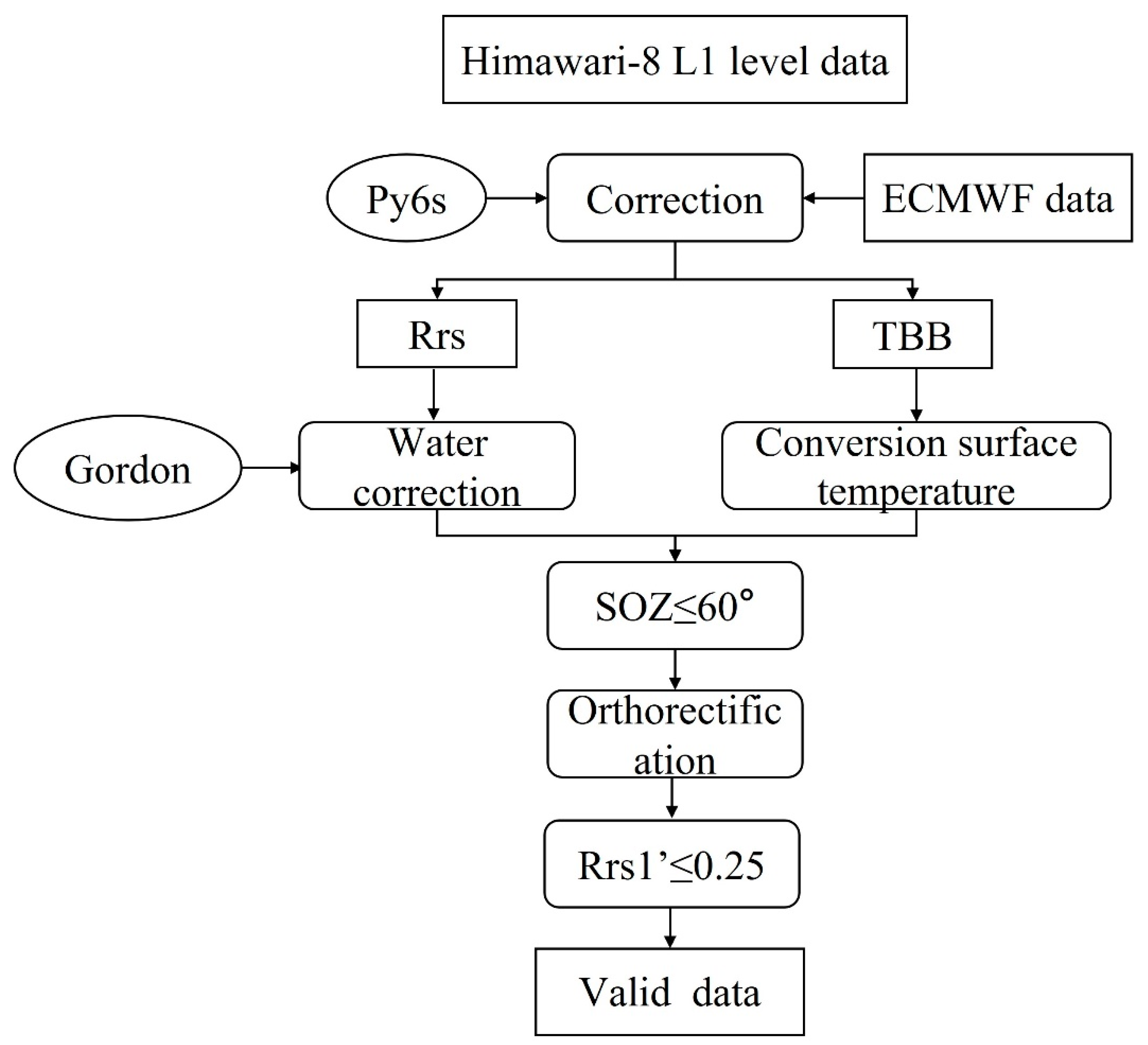
For H8′s L1-level data, we initially conducted atmospheric correction using the refined 6S model. Following correction, we applied the Gordon model to perform water body correction on the remote sensing R r s data. The corrected radiance temperature data were subsequently converted to surface temperature. Using Equations (2) and (3), the atmospherically corrected radiance temperature data were transformed into brightness temperature data. Equation (4) was employed to calculate the surface temperature data. Subsequently, the portion of R r s corresponding to SOZ of less than 60° was considered to be valid data. Equation (5) was applied to correct the R r s for bands 1 to 6, and ultimately, data with R r s 1 ≤ 0.25 were deemed valid. The specific flowchart is illustrated in Figure 1.

2.1.2. DO Data

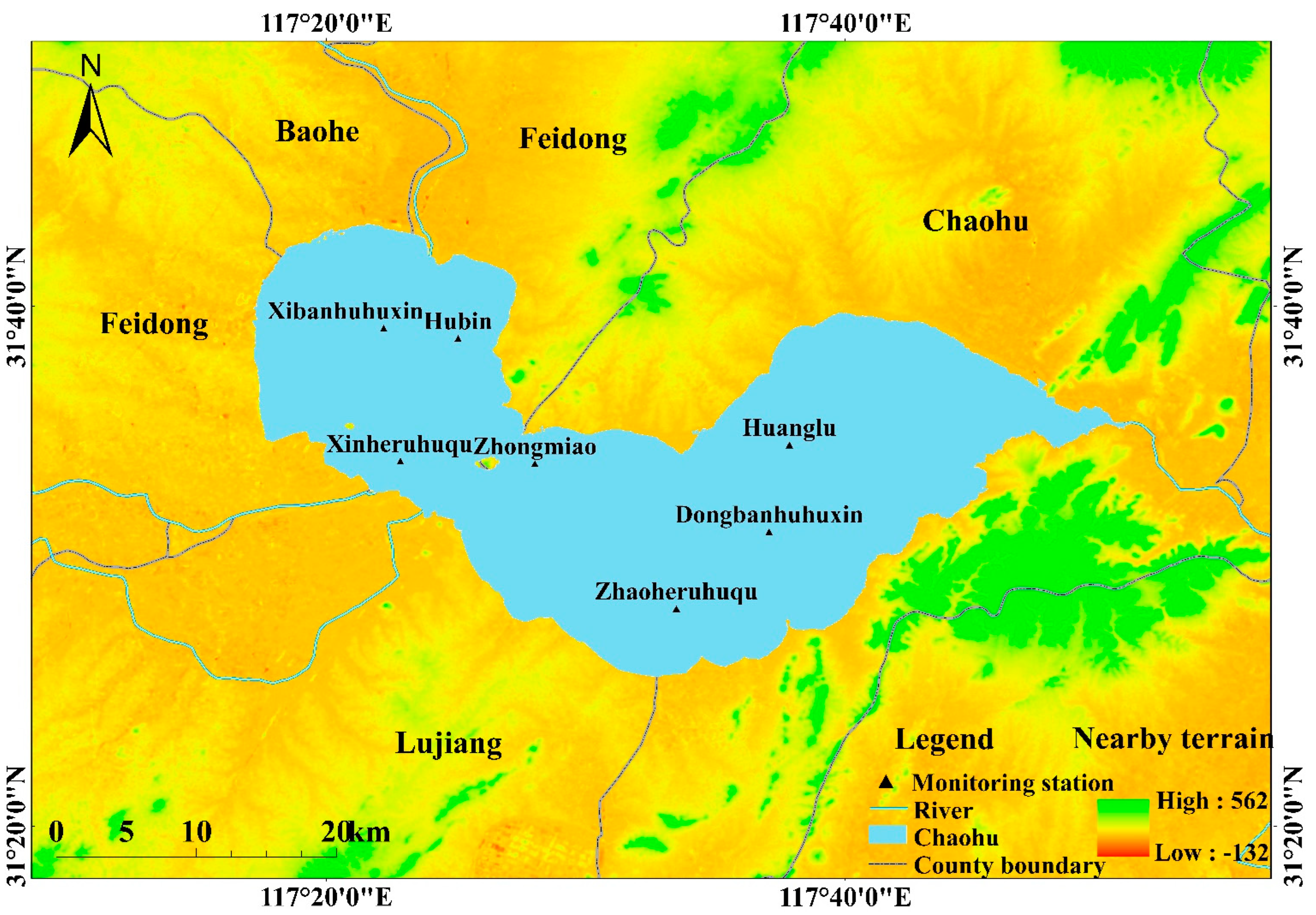
The measured water quality data used in this study are obtained from the National Surface Water Quality Automatic Monitoring Real-Time Data, which is a comprehensive business portal of the Ministry of Ecology and Environment for the “13th Five-Year Plan” period. The data collection follows the technical specifications of surface water automatic monitoring (HJ 915-2017). The DO data for the Lake Chaohu area from 2019 to 2021 are retrieved. Lake Chaohu (117°17′27.90″~117°50′35.78″ E, 31°42′40.87″~31°25′11.45″ N) is the fifth largest freshwater lake in China, located in the central part of Anhui Province. It has a lake area of approximately 800 km2 and a shoreline length of 181 km. The maximum water area is about 825 km2, with a maximum water storage capacity of 4.81 billion m3 and a maximum depth of 7.98 m. It serves as an important drinking water source for the cities of Hefei and Chaohu, playing a significant role in the economic development and modernization of Anhui Province. According to the “Surface Water Environmental Quality Standards” (GB3838-2002), the overall water quality of Lake Chaohu is classified as Class III, showing eutrophication, excessive levels of total phosphorus and total nitrogen, and frequent occurrences of cyanobacteria blooms. The spatial distribution of the monitoring sections within the Lake Chaohu region is shown in Figure 2. The monitoring time of the water quality automatic monitoring stations is used as the data annotation time, with a monitoring frequency of 1 h per measurement, and the unit is mg/L. In this study, seven valid monitoring sections with DO measurements are selected based on the coordinates determined in Section 2.1.1. The information of the monitoring sections is provided in Table 2.
Since automatic water quality monitoring stations may be influenced by environmental changes or instrument failures during data collection, it is necessary to handle missing and abnormal data to ensure the accuracy of the model’s fitted data. The missing values in the obtained DO data are removed, following the 3σ principle. Concentration data within the range of D O m e a n 3 × D O s t d , D O m e a n + 3 × D O s t d are retained as the actual DO data used in the model, while data outside this range are considered as abnormal and removed. Here, D O m e a n represents the average DO concentration of the current monitoring section, and D O s t d represents the standard deviation of the DO concentration of the current monitoring section.

2.1.3. ERA5 Reanalysis Data

ERA5 is the latest global reanalysis dataset of the atmosphere, land surface, and ocean by the ECMWF. It is the successor to ERA-Interim and provides a comprehensive collection of global meteorological, land, and ocean observations from 1979 to the present [31]. ERA5 incorporates global meteorological, land, and ocean observation data from 1979 to the present. Employing advanced physical processes and data assimilation techniques, ERA5 provides high-quality reanalysis of the atmosphere, land, and ocean. Reanalysis involves the use of modern analysis methods and meteorological models, combined with observational data and historical simulations, to generate a consistent series of historical meteorological data, encompassing various meteorological, land, and oceanic elements such as temperature, wind, precipitation, clouds, land surface temperature, and sea surface temperature. This fills in gaps in observations from the past. The temporal resolution is 1 h per time step, and the spatial resolution is 0.25°.
The ERA5 analysis dataset utilized in this study includes temperature at a height of 2 m, latent heat flux from the surface to the atmosphere, surface pressure, latent heat flux from the atmosphere to the surface, and total precipitation. Temperature in the atmosphere varies with altitude. Near the Earth’s surface, temperature is generally highest, gradually decreasing with increasing altitude. To better understand the actual temperature experienced by humans and surface ecosystems, “2 m temperature” is introduced. It represents the temperature measured at a height of 2 m above the ground. This is a reasonable choice, as at this height, temperature typically closely reflects the actual air temperature experienced by people. The latent heat flux from the surface to the atmosphere is an important concept described in meteorology and Earth science. It quantifies the heat released or absorbed during water phase transitions. Specifically, it refers to the heat released when water evaporates from a liquid state (such as surface water bodies or soil moisture) into water vapor, or the heat absorbed when water vapor condenses into liquid water. Conversely, the latent heat flux from the atmosphere to the surface refers to the heat either released when water vapor condenses into liquid water in the atmosphere or absorbed when water vapor falls to the surface and evaporates. Surface pressure refers to the atmospheric pressure at the Earth’s surface, and is often used to indicate the atmospheric pressure exerted on the Earth’s surface. Surface pressure is a crucial parameter in weather and climate research, playing a key role in predicting weather, analyzing meteorological phenomena, and studying atmospheric motions. Total precipitation refers to the accumulated amount of precipitation in a specific area over a given time period. The ERA5 reanalysis data used in this study was downloaded from https://cds.climate.copernicus.eu/cdsapp#!/dataset/reanalysis-era5-land?tab=form (accessed on 25 August 2022), in the format of NetCDF files.

2.2. Model Development and Performance Evaluation

2.2.1. Inversion Dataset

Firstly, based on the spatial and temporal fusion of the H8 calibration data and the measured dissolved oxygen data at each monitoring section of Chaohu Lake, the spatial and temporal fusion of the remote sensing data at 10 min intervals and the water quality data at 1 h intervals is carried out. To achieve the spatial and temporal fusion of water quality data and remote sensing data, the measured DO data from monitoring sections and the channel information and spectral indices of H8 data resolved using the same latitude and longitude coordinates are spatially fused. In terms of time, the shooting time of H8 images is synchronized with the time of DO measurements based on the lower frequency of water quality data (1 h per time step) to ensure consistent time scales. To develop a DO inversion model suitable for the entire lake region, the data from the seven effective monitoring sections in Lake Chaohu are combined, resulting in a total of 17,366 valid data points (N = 17,366). DO is considered to be the output data for the model. As each monitoring station is situated within a 2 × 2 km grid cell, this study treats the inverted DO concentration values as the average for individual measurement location grids. To maximize the utilization of remote sensing data, this study uses visible bands 1–6 and infrared bands 7–16 as input data for the model. Additionally, the time of each H8 observation is converted into cosine values and used as one of the input data [32]. For the date component, the following equation, Equation (6), is used to convert the date into cosine values:
c o s i n e t = cos ( 2 π d 365 )
where d represents the number of days in a year. The purpose of this formula is to convert the date into a cosine value with periodic characteristics, where the total number of days in a year is the length of the period. Since the date is a continuous variable throughout the year, converting it into a cosine value with periodic characteristics allows the model to better utilize the cyclic features of the date, such as seasonal variations. For the time component, the following Equation (7) is used to convert the time into cosine values:
c o s i n e t = cos 2 π s 86,400
where s represents the number of seconds in a day. The purpose of this formula is to convert the time into cosine values with periodic characteristics, where the total number of seconds in a day is the length of the period. Since time is a continuous variable within a day, converting it into cosine values with periodic characteristics allows the model to better utilize the cyclic features of time, such as daily peaks and troughs. In summary, the approach of converting date and time into cosine values helps the model better utilize the periodic characteristics in the time series data, thereby improving the predictive performance of the model.
In machine learning, proper dataset partitioning can improve training efficiency. Therefore, we divided the water quality inversion dataset, and 80% of the data was randomly allocated for training the model, while 20% of the data was used for model validation. We also normalized the training dataset using the following equation, Equation (8):
x   i = x i x ¯ σ  
In the equation, x   i represents the ith standardized variable of x; x i represents the ith variable of x; x ¯ represents the mean of the x variables; and σ represents the standard deviation of the x variables.

2.2.2. Model Selection

In this study, six machine learning algorithms, namely Multiple Linear Regression (MLR), Ridge Regression (RR) [33], Classification And Regression Tree (CDRT) [34], SVR [6], RF [24], and eXtreme Gradient Boosting tree (XGBoost) [35], were selected as comparative models for experimentation. The dataset was divided using a consistent method, and the grid search method (GridSearchCV) was employed to select the relatively optimal hyperparameters for each model.
Each machine learning algorithm has its own characteristics. Ridge Regression is a linear regression model that uses L2 regularization. By adding a regularization term to the loss function, it effectively avoids overfitting issues and improves the model’s generalization ability. Due to the L2 regularization, the RR algorithm can shrink coefficients, minimizing the impact of low correlation between variables on the model and reducing the model’s variance.
CDRT is a commonly used non-parametric regression model that can classify samples based on input features and generate a tree-like structure. It is easy to understand and interpret, providing an intuitive display of the relationships between features. CDRT does not require assumptions about data distribution, can handle non-linear problems, and is suitable for various types of data, displaying robustness.
SVR is a variation of Support Vector Machines (SVM) primarily used for regression problems. It maps data to a high-dimensional space through non-linear mapping, selects representative support vectors to construct the optimal hyperplane, and maximizes the margin between predicted values and true values. SVR exhibits strong robustness and the ability to handle non-linear problems, but it is sensitive to feature scaling. It requires selection of an appropriate kernel function and appropriate tuning parameters to optimize model performance.
RF is an ensemble learning method consisting of multiple decision trees. Each decision tree is built based on different random subsets of samples and random features. Predictions are made through voting or averaging. RF demonstrates robustness and the ability to handle high-dimensional data and non-linear problems effectively. It does not require preprocessing operations such as feature scaling or data standardization. RF is widely applied in various fields, including classification, regression, anomaly detection, and feature selection, and is considered a highly effective machine learning method.
XGBoost is an efficient implementation of the Gradient Boosting Regression Tree (GBRT) algorithm. It incorporates the gradient boosting idea, requiring less memory and operating at a faster speed compared to other implementations. XGBoost has gained popularity due to its high performance in various tasks.

2.2.3. Model Evaluation and Hyperparameter Tuning

To accurately assess the fitting and performance of the models, this study adopted three metrics as evaluation criteria: coefficient of determination (R2), root mean square error (RMSE), and mean absolute error (MAE). R2 is used to evaluate the agreement between the simulated values and the observed values of multiple variables. RMSE measures the deviation between the simulated values and the measured values, directly reflecting the dispersion of the simulated values around the measured values. MAE indirectly measures the accuracy of the model, with lower values indicating higher accuracy. The calculation formulas, ranges, and optimal values for these evaluation metrics are shown in Table 3. For the evaluation metrics, the GridSearchCV method was employed to perform hyperparameter tuning for each model, selecting the best parameters as fixed parameters for the models.

2.2.4. Correlation Analysis

To determine the influencing factors of DO concentration, this section conducts a Pearson correlation analysis between the overall DO concentration obtained from the RF model inversion for the Lake Chaohu region and specific ERA5 reanalysis data acquired in Section 2.1.3. To ensure data quality, we calculate the daily averages of the inverted overall DO concentration for the Lake Chaohu region and perform a Pearson correlation analysis with ERA5 reanalysis data. Prior to conducting the correlation analysis, we employ the variance inflation factor (VIF) for collinearity diagnosis of variables. If VIF < 10 [36], the variables pass the collinearity diagnosis, indicating the absence of collinearity issues.
V I F i = 1 1 R i 2
V I F i measures the variance inflation factor for the predictor variable X i to assess its multicollinearity with other predictor variables. R i 2 represents the coefficient of determination (R-squared value) when using X i as the response variable and other variables as feature variables in regression analysis. It quantifies the goodness of fit. A higher value of R i 2 corresponds to a larger V I F i value, indicating a more pronounced multicollinearity between the predictor variable Xi and other predictor variables.
r = 1 n 1 i = 1 n ( X i X ˉ s X ) ( Y i Y ˉ s Y )
r represents the simple correlation coefficient of the sample, where X i is the ith value of the first variable, Y i is the ith value of the second variable, X ˉ is the mean of the first variable X , Y ˉ is the mean of the variable Y , s X is the standard deviation of the first variable X , and s Y is the standard deviation of the second variable Y .

3. Results

3.1. Analysis of Measured DO Data

Figure 3 shows the monthly average time series trend of DO concentration at different monitoring sections from 2019 to 2021, and Figure 4 shows the seasonal average of DO concentration over the three years.
From the temporal distribution, as shown in Figure 3 and Table 4, it can be observed that the original DO concentration in Lake Chaohu exhibits significant seasonal variation. The MK trend test reveals that the overall DO concentration in spring (March to May) shows a decreasing trend (p < 0.01), while in autumn (September to November), it shows an increasing trend (p < 0.01). The DO concentration in summer (June to August) (8.19 ± 2.29 mg/L) is lower than in winter (December to February) (11.69 ± 1.02 mg/L), and it exhibits different trends among different years, indicating significant seasonal differences. The standard deviation of DO concentration is higher in summer and lower in winter, indicating larger fluctuations in DO during summer and smaller fluctuations during winter. In terms of annual variation, the minimum average DO concentration occurs in summer, while the maximum average occurs in winter, indicating an uneven distribution of DO concentration at the seasonal level and the significant influence of temperature.
From the spatial distribution, as shown in Figure 4 and Table 4, it can be observed that the section with the highest DO concentration in Lake Chaohu is Huanglu (11.88 ± 0.84 mg/L), while the section with the lowest DO concentration is Xinheruhuqu (7.52 ± 2.05 mg/L). The northeastern region of Lake Chaohu (Huanglu and Dongbanhuhuxin) generally has relatively higher DO concentrations, while the southern region (Zhaoheruhuqu) has relatively lower DO concentrations. The DO concentration is also relatively higher along the coastal areas (Hubin, Zhongmiao). The section with the highest standard deviation is Xinheruhuqu, likely due to multiple rivers flowing into this area, resulting in larger fluctuations in DO concentration compared to other sections.

3.2. Model Performance

Pearson correlation analysis was used to compare the correlation between all remote sensing features and DO concentration. Table 5 presents the Pearson correlation coefficients between various features and the measured DO data, indicating the feasibility of using remote sensing information such as visible, near-infrared, and shortwave infrared bands of R r s , infrared bands of surface temperature, and cosine values of time for DO concentration inversion.
The MLR model, as a linear regression model, lacks direct tunable hyperparameters. The linear_model.LinearRegression model from the scikit-learn library in Python was directly employed for computations, yielding a linear regression equation of y = 0.725 x + 2.75. The optimal results for the remaining five machine learning models after hyperparameter tuning using GridSearchCV are presented in Table 6.
The evaluation results of the models on the test set, representing the performance of the models in practical applications, are shown in Table 7 and Figure 5. The RF model performs the best in DO inversion, with a high R2 score of 0.84 and low RMSE and MAE values of 0.69 and 0.54, respectively, indicating accurate prediction of DO concentration. The SVR model (R2 = 0.72, RMSE = 0.89, MAE = 0.67) and XGBoost model (R2 = 0.83, RMSE = 0.70, MAE = 0.54) also show good performance. The CDRT model has moderate accuracy, with an R2 score of 0.62 and relatively low RMSE and MAE values. However, the MLR and RR models perform the worst, with an R2 score of only 0.43 and higher RMSE and MAE values. The RF model shows an average improvement of 38% in R2, a 13% reduction in RMSE, and a 33% reduction in MAE compared to other models, indicating its effectiveness in DO inversion.
To further validate the performance of RF, we compared the measured DO and estimated DO for each season. As shown in Figure 6, the model performed poorly in the spring season, and DO values in the range of 7–13 mg/L were observed. The spring season was characterized by significant temperature changes, which in turn affected the release rate of oxygen in the lake. The DO concentration varied accordingly. Spring is also a season with relatively high rainfall in the Jianghuai region of China, leading to a large influx of rainwater and runoff into Lake Chaohu. This increases the flow rate of the lake water, and it is also the traditional production season for aquaculture in Lake Chaohu, resulting in a higher discharge of aquaculture waste and a larger range of DO concentration variations.
To validate the accuracy of the RF model in long-term sequence applications, this study sequentially calculated the monthly average values for the observed data from seven monitoring stations. The monthly average values of each station were further averaged across all seven stations, with the results serving as the observed monthly average DO concentration for the entire Lake Chaohu region. Using the trained RF model and H8 satellite data, the DO concentrations for each 2 × 2 km grid cell were inverted. The inverted DO concentrations were then averaged across all grid cells fully within the lake to obtain the overall inverted DO concentration for the Lake Chaohu region. Subsequently, the time-series inverted DO concentration values were averaged on a monthly basis to derive the inverted monthly average DO concentration for the Lake Chaohu region. To assess the accuracy of the inversion, a comparison was made with the observed monthly average DO concentrations. The comparison results are shown in Figure 7; the trends of the inverted and observed monthly average values generally aligned. The errors between the inverted and observed monthly average values remained within 1 mg/L. Notably, the RF model tended to overestimate or underestimate high and low values, especially at extreme points, indicating a need for further improvement in the RF model. Nevertheless, the overall error was relatively small.

3.3. DO Spatio-Temporal Distribution

In this study, using H8 data from 2019 to 2021 and the optimized RF model, the grid-based DO concentrations in the entirety of Lake Chaohu were re-estimated. The results are shown in Figure 8. The lake was divided into three parts: northwest, central-south, and northeast. The analysis revealed that the average annual DO concentration in Lake Chaohu decreased by 1.4% and 0.9% in 2020 and 2021, respectively, compared to 2019. Regarding the intra-annual variations, the overall DO concentration in Lake Chaohu showed a decreasing trend followed by an increasing trend. Generally, DO concentration started to decline from January to July, reaching its lowest point, and then began to rise from August to September. Subsequently, a brief decline occurred in October to November, followed by a gradual increase from December to the next January, reaching the highest value. The variation in DO concentration exhibited seasonal differences, with the highest concentrations observed in winter and the lowest concentrations observed in summer and autumn. In terms of spatial distribution, the DO concentrations in Lake Chaohu were uneven. From 2019 to 2021, the annual average DO concentrations in the northwest, central-south, and northeast regions of Lake Chaohu were 10.12 mg/L, 9.98 mg/L, and 9.96 mg/L, respectively. Therefore, it can be concluded that the DO concentration in the northwest region of Lake Chaohu is higher than that in the central-south and northeast regions.

3.4. The Factors Influencing DO Concentration

Combined with the ERA5 data analyzed near Lake Chaohu, Pearson correlation analysis was performed on the inversion results of DO concentration in the Lake Chaohu region from 2019 to 2021. All variables passed the collinearity test, with VIF values less than 10, as shown in Table 8. The results of the correlation analysis are presented in Table 9. Among the correlation indicators, DO showed a significant negative correlation with temperature, with a correlation coefficient of −0.615. Surface pressure, latent heat flux from the atmosphere to the surface, and latent heat flux from the surface to the atmosphere followed as the next important factors, with correlation coefficients of 0.583, −0.480, and 0.444, respectively. The significance level (P) for all correlations was less than 0.01, indicating that temperature is the main factor influencing dissolved oxygen. Typically, an increase in the latent heat flux from the atmosphere to the surface results in higher water temperature on the lake surface, which leads to a decrease in the solubility of dissolved oxygen in the water.

4. Discussion

4.1. Limitations of the Model

The results obtained from the model in this study may have some discrepancies with the actual values, which can be attributed to various factors. Firstly, the water quality parameters are collected from fixed monitoring points, while the remote sensing satellite data used in the study has a relatively low spatial resolution (2 km). This can lead to the presence of other interfering factors within the same remote sensing pixel, making it challenging to achieve a perfect match. Secondly, the DO concentrations outputted by the proposed DO inversion model represent the average concentration within a remote sensing pixel, which may not directly correspond to the levels measured by automatic monitoring stations. The proximity to land and the influence of the nearshore effect [37] can also impact the accuracy of the inversion results, with the performance being less satisfactory in areas closer to the lake’s shoreline [15]. Furthermore, the real-time water quality measurements taken at automatic monitoring stations may be affected by unexpected events such as changes in sensor environment, network failures, or the passage of vessels and fish schools. Additionally, remote sensing satellites are unable to capture the vertical profiles of water bodies, and different water bodies exhibit significant individual variations in their optical properties. All these factors can introduce certain errors in water quality inversion and prediction.
The models were exclusively trained on data from the Lake Chaohu region. Due to the pronounced spatiotemporal heterogeneity of water quality, if extended to monitor other water bodies, in order to adapt the model to varying data dynamics, it would be imperative to retrain the model and adjust hyperparameters based on the actual DO measurements and remote sensing data specific to the water body’s region. This necessitates re-calibrating the model to ensure its efficacy and accuracy under differing conditions.

4.2. Analysis of DO Spatial and Temporal Distribution in Lake Chaohu

Studying the spatial and temporal distribution of DO in lakes is essential for gaining a deeper understanding of the state and changes in lake ecosystems and providing scientific basis and guidance for lake management and protection. DO is a vital requirement for the survival and reproduction of aquatic organisms, and the spatial and temporal distribution of DO in lake water can influence the structure and functioning of lake ecosystems. Low DO concentrations can result in the death of aquatic organisms, population decline, and reduced species diversity [38]. Oxygen deficiency in water bodies can also lead to increased phosphorus release flux from sediments and reduced efficiency of inorganic nitrogen removal, leading to persistent eutrophication and posing risks to ecosystem integrity [39]. From the analysis of the temporal characteristics of DO in Lake Chaohu, it can be observed that DO concentrations are significantly lower in the summer and autumn seasons compared to the spring and winter seasons. Generally, higher water temperatures correspond to lower-saturation DO concentrations in water bodies. In the summer and autumn seasons, water temperatures are higher, resulting in lower DO concentrations, while in the spring and winter seasons, water temperatures are lower, leading to higher DO concentrations. This finding is consistent with previous studies [40]. In terms of spatial distribution, Xinheruhuqu is closer to the urban area. On one hand, the increased presence of vegetation and higher photosynthetic efficiency near urban areas, which are influenced by urbanization, can contribute to higher DO concentrations. Moreover, water bodies around urban areas often experience pollution from urban discharge, such as organic matter, nitrogen, and phosphorus. These pollutants are carried away by water flow, reducing organic matter content in the water and consequently increasing DO concentrations. Additionally, water flow can bring in air and oxygen, further enhancing DO concentrations in the water. Overall, understanding the spatial and temporal distribution of DO in Lake Chaohu provides valuable insights into the lake’s ecological status and dynamics. It highlights the importance of considering seasonal variations, water temperature, urban influence, and water flow dynamics when assessing and managing lake ecosystems.

4.3. Analysis of Factors Affecting DO Concentration

We conducted a correlation analysis between daily average DO concentration and five climate factors: temperature, latent heat flux from the land surface to the atmosphere, surface air pressure, latent heat flux from the atmosphere to the land surface, and precipitation. This analysis aimed to investigate the impact of different climate factors on DO concentration in Lake Chaohu. The results indicate that temperature is the primary factor influencing DO concentration, followed by surface air pressure. These findings align with previous studies [8,41]. When temperature increases, the molecular kinetic energy in the liquid phase rises, weakening the intermolecular interactions. This accelerates the rate at which oxygen molecules escape from the water, leading to a decrease in DO concentration. At the water’s surface, gas exchange occurs between the water and the atmosphere, with oxygen being one of the gases involved. When atmospheric pressure increases, oxygen dissolves more readily into the water because dissolved oxygen exists in equilibrium between the gas and liquid phases. Consequently, as atmospheric pressure increases, the concentration of dissolved oxygen in the water also increases. According to Henry’s law [42], the solubility of a gas in a liquid is directly proportional to the partial pressure of the gas at a given temperature. Therefore, when atmospheric pressure increases, the DO concentration in the water also increases. Additionally, water movement and turbulence enhance the diffusion of oxygen between water and air, thereby increasing the DO concentration. Furthermore, flowing water can mix oxygen-rich water with water that has a lower oxygen content, thereby raising the overall DO concentration in the water body. On the other hand, hydrodynamics can also influence the consumption of DO concentration. For example, in turbulent flows, aquatic organisms are more active and have a higher respiration rate, resulting in greater oxygen consumption. In such cases, the DO concentration may decrease. Therefore, hydrodynamic factors can affect the DO concentration in water bodies. In the management and protection of water bodies, it is crucial to consider the influence of hydrodynamic factors to ensure that the DO concentration meets the biological requirements while maintaining a healthy aquatic ecosystem.

4.4. Prospective Nature of the Model

When selecting satellite data products, we often face a trade-off between spatial and temporal resolution. In this study, although we utilized satellite data products with a 2 km spatial resolution and excellent temporal resolution, we unavoidably encountered some loss of spatial information. This scenario is common in practical applications, as there is rarely a single data source that can provide both high spatial resolution and high temporal resolution simultaneously.
However, to address this trade-off, the consideration of synergy models or data fusion techniques is suggested. The core idea of these approaches is to integrate information from different data sources to compensate for their individual limitations. By combining high-spatial-resolution data and high-temporal-resolution data, we can anticipate more accurate results in both space and time dimensions. Synergy models can leverage the strengths of diverse datasets to provide comprehensive information and enhance predictive accuracy.
Data fusion techniques can also mitigate the constraints arising from the spatial–temporal trade-off to a certain extent. By merging data from various sources, we can exploit their complementarity to obtain more comprehensive observational information. This can be achieved through a range of algorithms and methods, including weighted fusion and model-based fusion.
Introducing the topic of synergy models or data fusion in the discussion can showcase our consideration and the forward-thinking nature of the study. While our research employed specific data sources, this does not imply that we are confined to those methods alone for enhancing model accuracy and reliability. By harnessing the strengths of different data sources, we have the opportunity to provide innovative solutions to address the challenges posed by spatial–temporal trade-offs.

5. Conclusions

With the rapid development of artificial intelligence and remote sensing technology, applying machine learning models to the inversion and prediction of water quality in inland lakes has become a hot topic in the interdisciplinary field of artificial intelligence and the environment. In this study, by utilizing a large amount of historical water quality monitoring data and satellite remote sensing data, we have implemented increasingly frequent and macroscopic monitoring activities using machine learning models. This approach has the advantages of wide coverage and rapid monitoring, providing an effective reference for improving the level of water environment monitoring and holding significant implications for the protection of lake water quality. The main conclusions drawn from this research are as follows:
(1)
Based on the statistical analysis of measured DO data, it can be observed that Lake Chaohu exhibits distinct seasonal variations in DO concentration over time. The MK trend test indicates that the overall DO concentration in spring shows a significant decreasing trend (p < 0.01), while the DO concentration in autumn shows a significant increasing trend (p < 0.01). The DO concentration in summer (8.19 ± 2.29 mg/L) is lower than in winter (11.69 ± 1.02 mg/L), and the trends vary among different years, showing significant seasonal differences. The standard deviation of DO is higher in summer and lower in winter, indicating greater fluctuations in DO during summer and smaller fluctuations during winter. In terms of spatial distribution, the section with the highest DO concentration in Lake Chaohu is Huanglu (11.88 ± 0.84 mg/L), while the section with the lowest DO concentration is the area of Xinheruhuqu (7.52 ± 2.05 mg/L). The northeastern region of Lake Chaohu (Huanglu and Dongbanhuhuxin) generally exhibits relatively high DO concentrations, while the southern region (Zhaoheruhuqu) generally exhibits relatively low DO concentrations. Additionally, the coastal areas (Hubin and Zhongmiao) also have relatively high DO concentrations.
(2)
By using H8 synchronous satellite data and comparing various machine learning models, it is found that the Random Forest (RF) model performs the best in DO inversion, with an R2 of 0.84, RMSE of 0.69, and MAE of 0.54. These results outperform other models, showing a 38% improvement in average R2, a 13% decrease in RMSE, and a 33% decrease in MAE. This indicates that the model can accurately predict DO concentration.
(3)
Based on the well-trained RF model and H8 data, the overall DO concentration in Lake Chaohu from 2019 to 2021 was re-inverted. The results show seasonal variations in DO concentration, with the highest concentrations occurring in winter and the lowest in summer and autumn. From 2019 to 2021, the annual average DO concentrations in the northwest, central-south, and northeast regions of Lake Chaohu were 10.12 mg/L, 9.98 mg/L, and 9.96 mg/L, respectively. It can be concluded that the DO concentration in the northwest region of Lake Chaohu is higher than that in the central-south and northeast regions.
(4)
Combined with ERA5 data and the inverted DO data, the results indicate a significant negative correlation between DO and temperature, with a correlation coefficient of −0.615. Surface air pressure, latent heat flux from the atmosphere to the land surface, and latent heat flux from the land surface to the atmosphere are the next significant factors influencing DO concentration, with correlation coefficients of 0.583, −0.480, and 0.444, respectively. The p-values for the correlations are all less than 0.01.

Author Contributions

Methodology, K.S. and H.Y.; software, P.W.; validation, Q.L., H.W. and G.C.; formal analysis, P.W.; investigation, K.S.; resources, Q.L.; data curation, H.Y.; writing—original draft preparation, P.W.; writing—review and editing, H.W.; funding acquisition, Q.L. All authors have read and agreed to the published version of the manuscript.

Funding

This research was funded by State key laboratory of plateau ecology and agriculture, Qinghai university: Self-Occupancy Issue Fund(2023-ZZ-09) and the National Key Research and Development Program (2021YFC310170504).

Data Availability Statement

The data presented in this study are available on request from the corresponding authors. The data are not publicly available due to the continuation of a follow-up study by the authors.

Conflicts of Interest

The authors declare no conflict of interest.

References

  1. Xu, W.Y.; Sheng, T.; Liu, S.; Gao, H.W. Water quality detection system based on multi-wavelength spectral snsors. Foreign Electron. Meas. Technol. 2022, 41, 112–116. [Google Scholar]
  2. Wang, S.M.; Qin, B.Q. Research Progress on Remote Sensing Monitoring of Lake Water Quality Parameters. Environ. Sci. 2022, 44, 1228–1243. [Google Scholar]
  3. Huang, D.L.; Ni, Z.K.; Zhao, S.; Zhang, B.T.; Feng, M.L.; Chen, H.W.; Li, X.X.; Wang, S.R. Correlation Analysis of Water Quality between Lake Inflow and Outflow: A Case Study of Poyang Lake. Environ. Sci. 2019, 40, 4450–4460. [Google Scholar]
  4. Cheng, C.M.; Wei, Y.C.; Lv, G.N.; Yuan, Z.J. Remote estimation of chlorophyll-a concentration in turbid water using a spectral index: A case study in Taihu Lake, China. Environ. Monit. Assess. 2019, 191, 84. [Google Scholar]
  5. Zhang, H.J.; Wang, B.; Zhou, J.; Yu, Y.; Ke, S.; Huang, F.K. Remote sensing retrieval of inland river water quality based on BP neural network. J. Cent. China Norm. Univ. (Nat. Sci.) 2021, 56, 333–341. [Google Scholar]
  6. Guo, H.W.; Huang, J.J.; Zhu, X.T.; Wang, B.; Tian, S.; Xu, W. A generalized machine learning approach for dissolved oxygen estimation at multiple spatiotemporal scales using remote sensing. Environ. Pollut. 2021, 28, 11734. [Google Scholar]
  7. Chi, L.B.; Song, X.X.; Yuan, Y.Q.; Wang, W.T.; Cao, X.H.; Wu, Z.X.; Yu, Z.M. Main factors dominating the development, formation and dissipation of hypoxia off the Changjiang Estuary (CE) and its adjacent waters, China. Environ. Pollut. 2020, 265, 115066. [Google Scholar]
  8. Wang, J.; Wu, Q.; Luo, H.; Sun, L.L.; Li, N.; He, Y.Q. Study on the Spatial-temporal Distribution and Influencing Factors of Dissolved Oxygen in the North Main Stream of Dongjiang River. J. Yangtze River Sci. Res. Inst. 2023, 1–8. [Google Scholar]
  9. Kim, Y.H.; Son, S.; Kim, H.C.; Kim, B.; Park, Y.G.; Nam, J.; Ryu, J. Application of satellite remote sensing in monitoring dissolved oxygen variabilities: A case study for coastal waters in Korea. Environ. Int. 2020, 134, 105301. [Google Scholar]
  10. Sagan, V.; Peterson, K.T.; Maimaitijiang, M.; Sidike, P.; Sloan, J.; Greeling, B.A.; Maalouf, S.; Adams, C. Monitoring inland water quality using remote sensing: Potential and limitations of spectral indices, bio-optical simulations, machine learning, and cloud computing. Earth-Sci. Rev. 2020, 205, 103187. [Google Scholar]
  11. Karakaya, N.; Evrendilek, F. Monitoring and validating spatio-temporal dynamics of biogeochemical properties in Mersin Bay (Turkey) using Landsat ETM+. Environ. Monit. Assess. 2011, 181, 457–464. [Google Scholar] [PubMed]
  12. El Din, S.E.; Zhang, Y.; Suliman, A. Mapping concentrations of surface water quality parameters using a novel remote sensing and artificial intelligence framework. Int. J. Remote Sens. 2017, 38, 1023–1042. [Google Scholar]
  13. Batur, E.; Maktav, D. Assessment of Surface Water Quality by Using Satellite Images Fusion Based on PCA Method in the Lake Gala, Turkey. IEEE Trans. Geosci. Remote Sens. 2019, 57, 2983–2989. [Google Scholar]
  14. Yang, H.B.; Du, Y.; Zhao, H.L.; Chen, F. Water Quality Chl-a Inversion Based on Spatio-Temporal Fusion and Convolutional Neural Network. Remote Sens. 2022, 14, 1267. [Google Scholar]
  15. Zhao, X.L.; Xu, H.L.; Ding, Z.B.; Wang, D.Q.; Deng, Z.D.; Wang, Y.; Wu, T.F.; Li, W.; Lu, Z.; Wang, G.Y. Comparing deep learning with several typical methods in prediction of assessing chlorophyll-a by remote sensing:a case study in Taihu Lake, China. Water Supply 2021, 21, 3710–3724. [Google Scholar]
  16. Chen, J.; Quan, W.T. Using Landsat/TM Imagery to Estimate Nitrogen and Phosphorus Concentration in Taihu Lake, China. IEEE J. Sel. Top. Appl. Earth Obs. Remote Sens. 2012, 5, 273–280. [Google Scholar]
  17. Bessho, K.; Date, K.; Hayashi, M. An Introduction to Himawari-8/9-Japan’s New-Generation Geostationary Meteorological Satellites. J. Meteorol. Soc. Jpn. 2016, 94, 151–183. [Google Scholar]
  18. Taniguchi, N.; Kida, S.; Sakuno, Y.; Mutsuda, H.; Syamsudin, F. Short-Term Variation of the Surface Flow Pattern South of Lombok Strait Observed from the Himawari-8 Sea Surface Temperature. Remote Sens. 2019, 11, 1491. [Google Scholar]
  19. Torres, R.B.; Blanco, A.C. Preliminary Investigation on Chlorophyll-a And Total Suspended Matter Concentration in Manlia Bay Using Himawari-8 AHI and Sentinel-3 Olci C2rcc. Int. Arch. Photogramm. Remote Sens. Spat. Inf. Sci. 2021, XLVI-4/W6-2021, 303–311. [Google Scholar]
  20. Wu, W.X.; Wu, Y.L.; Jiang, P.; Ning, H.T. Depth neural network method for PM2.5 concentration estimation of Himawari-8 satellite based on ground air decoupling. Acta Sci. Circumstantiae 2021, 41, 1753–1763. [Google Scholar]
  21. Wang, G.; Wang, D.Y.; Wu, R. Application study of Himawari-8/AHI infrared spectral data on precipitation signal recognition and retrieval. Infrared Millim. Waves 2020, 39, 251–262. [Google Scholar]
  22. Ning, H.T.; Jiang, P.; Wu, Y.L. Research on Aerosol Optical Depth Retrieval of Himawari-8 Data Based on Deep Neural Networks. Adm. Techn. Environ. Monit. 2021, 33, 8–12. [Google Scholar]
  23. Wagle, N.; Acharya, T.D.; Lee, D.H. Comprehensive Review on Application of Machine Learning Algorithms for Water Quality Parameter Estimation Using Remote Sensing Data. Sens. Mater. 2020, 32, 3879–3892. [Google Scholar] [CrossRef]
  24. Liu, H.; Yu, T.; Hu, B.L.; Hou, X.S.; Zhang, Z.F.; Liu, X.; Liu, J.C.; Wang, X.J.; Zhong, J.J.; Tan, Z.X. UAV-Borne Hyperspectral Imaging Remote Sensing System Based on Acousto-Optic Tunable Filter for Water Quality Monitoring. Remote Sens. 2021, 13, 4069. [Google Scholar] [CrossRef]
  25. Xu, J.L.; Xu, Z.; Kuang, J.J.; Lin, C.; Xiao, L.H.; Huang, X.S.; Zhang, Y.F. An Alternative to Laboratory Testing: Random Forest-Based Water Quality Prediction Framework for Inland and Nearshore Water Bodies. Water 2021, 13, 3262. [Google Scholar] [CrossRef]
  26. Liu, Z.; Zhao, W.L.; Tian, X.Q.; Sang, Y.Y.; Qu, Y.L.; Ren, J.J.; Li, C.C. Retrieval of Ground PM2.5 Concentrations in Eastern China Using Data from Himawari-8 Satellite. Acta Sci. Nat. Univ. Pekin. 2022, 58, 443–452. [Google Scholar]
  27. Li, Y.; Yu, W. Study on average solar spectral irradiance based on FY-4 AGRI and Himawari-8 AHI. Mod. Electron. Tech. 2020, 43, 9–12,17. [Google Scholar]
  28. Gordon, H.R.; Wang, M. Retrieval of water-leaving radiance and aerosol optical thickness over the oceans with SeaWiFS: A preliminary algorithm. Appl. Opt. 1994, 33, 443–452. [Google Scholar] [CrossRef]
  29. Chen, J.; Zheng, W.; Wu, S.; Liu, C.; Yan, H. Fire Monitoring Algorithm and Its Application on the Geo-Kompsat-2A Geostationary Meteorological Satellite. Remote Sens. 2022, 14, 2655. [Google Scholar] [CrossRef]
  30. Qi, L.; Hu, C.M.; Duan, H.T.; Cannizzaro, J.; Ma, R.H. A novel MERIS algorithm to derive cyanobacterial phycocyanin pigment concentrations in a eutrophic lake: Theoretical basis and practical considerations. Remote Sens. Environ. 2014, 154, 298–317. [Google Scholar] [CrossRef]
  31. Hersbach, H.; Bell, B.; Berrisford, P.; Hirahara, S.; Horanyi, A.; Munoz-Sabater, J.; Nicolas, J.; Peubey, C.; Radu, R.; Schepers, D.; et al. The ERA5 global reanalysis. Q. J. R. Meteorol. Soc. 2020, 146, 1999–2049. [Google Scholar] [CrossRef]
  32. Thomakos, D. Smoothing Non-Stationary Time Series Using the Discrete Cosine Transform. J. Syst. Sci. Complex. 2016, 29, 382–404. [Google Scholar] [CrossRef]
  33. Zhang, Z.T.; Wang, H.F.; Karnieli, A.; Chen, J.Y.; Han, W.T. Inversion of Soil Moisture Content from Hyperspectra Based on Ridge Regression. J. Agric. Mach. 2018, 49, 240–248. [Google Scholar]
  34. Sun, D.L.; Yu, Y.Y. Goldberg M D. Deriving Water Fraction and Flood Maps from MODIS Images Using a Decision Tree Approach. IEEE J. Sel. Top. Appl. Earth Obs. Remote Sens. 2011, 4, 814–825. [Google Scholar] [CrossRef]
  35. Cao, Z.G.; Ma, R.H.; Duan, H.T.; Pahlevan, N.; Melack, J.; Shen, M.; Xue, K. A machine learning approach to estimate chlorophyll-a from Landsat-8 measurements in inland lakes. Remote Sens. Environ. 2020, 248, 111974. [Google Scholar] [CrossRef]
  36. Ma, P.W. Diagnosis and Empirical Analysis on Multicollinearity in Linear Regression Model. J. Huazhong Agric. Univ. Soc. Sci. Ed. 2008, 2, 78–81+85. [Google Scholar]
  37. Sun, X.; Zhang, Y.; Shi, K.; Zhang, Y.B.; Li, N.; Wang, W.J.; Huang, X.; Qin, B.Q. Monitoring water quality using proximal remote sensing technology. Sci. Total Environ. 2022, 803, 149805. [Google Scholar] [CrossRef]
  38. Wang, H.X.; Chu, X.Y.; Chen, Y.; Xu, L.; Yang, K. A study on temporal and spatial distribution characteristics of dissolved oxygen in surface water of megacities. Journal of East China Norm. Univ. (Nat. Sci.) 2020, 6, 154–163. [Google Scholar]
  39. Zhu, L.; Shi, W.Q.; Dam, B.V.; Kong, L.W.; Yu, J.H.; Qin, B.Q. Algal Accumulation Decreases Sediment Nitrogen Removal by Uncoupling Nitrification-Denitrification in Shallow Eutrophic Lakes. Environ. Sci. Technol. 2020, 54, 6194–6201. [Google Scholar] [CrossRef]
  40. Xie, F.Z.; Liu, Z.; Luo, K. Long Term Comprehensive Evaluation of Temporaland Spatial Variation of Water Quality in ChaohuLake, China. Pol. J. Environ. Stud. 2022, 31, 4383–4397. [Google Scholar] [CrossRef]
  41. Yang, C.; Fu, Y.Y.; Yang, Y.M.; Li, W.W. Evaluation of Dissolved Oxygen in Qinhuangdao Bathing Beach and Analysis of Its Influencing Factors. Sci. Technol. Innov. 2021, 25, 70–72. [Google Scholar]
  42. Sander, R.; Acree, W.E.; De Visscher, A.; Schwartz, S.E.; Wallington, T.J. Henry’s law constants (IUPAC Recommendations 2021). Pure Appl. Chem. 2022, 94, 71–85. [Google Scholar] [CrossRef]
Figure 1. Data processing flowchart.
Water 15 03081 g001
Figure 2. Chaohu DO concentration monitoring section map.
Water 15 03081 g002
Figure 3. Time-series trends of DO concentration in different sections of Lake Chaohu.
Water 15 03081 g003
Figure 4. Seasonal variation of DO concentration at different sections of Lake Chaohu.
Water 15 03081 g004
Figure 5. Fitting line plot of the DO inversion model in Lake Chaohu.
Water 15 03081 g005
Figure 6. RF model fit by season.
Water 15 03081 g006
Figure 7. Comparison graph of observed and inverted monthly average values for Lake Chaohu.
Water 15 03081 g007
Figure 8. The time-series graph shows the DO inversion results for Chaohu Lake from 2019 to 2021.
Water 15 03081 g008
Table 1. Himawari-8/AHI Channels 1 to 16: Parameters.
BandCenter Wavelength/μmPrimary Functions of Each Channel
R r s _010.46Vegetation, Aerosol Observation, Color Image Synthesis
R r s _020.51Vegetation, Aerosol Observation, Color Image Synthesis
R r s _030.64Lower Cloud (Fog) Observation, Color Image Synthesis
R r s _040.86Vegetation, Aerosol Observation
R r s _051.6Identification of Various Cloud Phases
R r s _062.3Observation of Cloud Droplet Effective Radius
tbb_073.9Observation of Lower Clouds (Fog), Natural Disasters
tbb_086.2Observation of Upper- and Middle-Level Water Vapor Content
tbb_097.0Observation of Middle-Level Water Vapor Content
tbb_107.3Observation of Middle- and Lower-Level Water Vapor Content
tbb_118.6Cloud Phase Identification and SO2 Monitoring
tbb_129.6Measurement of Total Ozone Amount
tbb_1310.4Observation of Cloud Images and Cloud Top Conditions
tbb_1411.2Observation of Cloud Images and Sea Surface Temperature
tbb_1512.3Observation of Cloud Images and Sea Surface Temperature
tbb_1613.3Measurement of Cloud Layer Height
Table 2. Information for each monitoring section in Chaohu Lake.
Monitoring SectionsLongitude and LatitudeTime Span or Time Period
Dongbanhuhuxin117.62° E, 31.522° N1 January 2019–31 December 2021
Hubin117.4203° E, 31.6461° N
Huanglu117.6331° E, 31.5778° N
Xibanhuhuxin117.3725° E, 31.6527° N
Xinheruhuqu117.3832° E, 31.5674° N
Zhaoheruhuqu117.5605° E, 31.4726° N
Zhongmiao117.4696° E, 31.5658° N
Table 3. Model evaluation metrics.
Model Evaluation MetricsComputational FormulaValue RangeBest Value
R2 R 2 = 1 i = 1 n ( y i y ^ ) 2 i = 1 n ( y i y ¯ ) 2 [0,1]1
RMSE R M S E = 1 n i = 1 n ( y i y ^ ) 2 [0,+∞]0
MAE M A E = 1 n i = 1 n y i y ^ [0,+∞]0
Notes: In the table, R 2 represents the coefficient of determination between the simulated values and the measured values. y i represents the i-th feature of the measured water quality variable, y ¯ represents the mean value of the measured water quality variable, y i ^ represents the simulated value of the i-th feature of the water quality variable, and n represents the sample size.
Table 4. Seasonal average values and standard deviations at different sections of Lake Chaohu. (DO/(mg/L)).
SectionSpringSummerAutumnWinterEntire Year
MeanStdMeanStdMeanStdMeanStdMeanStd
Chaohu9.971.768.192.299.041.7811.691.029.682.20
Dongbanhuhuxin10.221.728.242.068.931.6411.810.819.832.13
Hubin9.801.908.502.669.261.9011.611.089.742.28
Huanglu10.171.648.462.148.991.4211.880.849.842.04
Xibanhuhuxin9.742.068.352.499.252.0711.641.159.692.35
Xinheruhuqu9.931.737.522.058.771.8511.841.399.462.38
Zhaoheruhuqu10.011.567.941.888.951.5011.660.849.542.04
Zhongmiao9.921.568.382.529.091.9011.440.879.702.14
Table 5. The Pearson correlation coefficients between DO and various features.
FeaturesPearsonFeaturesPearson
R r s _01−0.10 **tbb_100.05
R r s _02−0.12 **tbb_11−0.24 **
R r s _03−0.21 **tbb_12−0.30 **
R r s _04−0.01tbb_13−0.23 **
R r s _05−0.06 **tbb_14−0.21 **
R r s _06−0.07 **tbb_15−0.17 **
tbb_07−0.31 **tbb_16−0.20 **
tbb_080.04 **cos_day0.32 **
tbb_090.05 **cos_hour−0.15 **
Note: ** indicates a significant correlation (at a two-tailed significance level of 0.01) based on Pearson correlation analysis.
Table 6. Optimal values of hyperparameters for each model.
ModelOptimal Values of Hyperparameters
RRalpha = 0.20
CDRTMax_depth = 9, Min_samples_split = 2, Min_samples_leaf = 1
SVRkernel = ‘rbf’, C = 100
RFMax_depth = 50, n_estimators = 900, max_features = 5, min_samples_split = 2, min_samples_leaf = 1
XGBoostn_estimators = 900, max_depth = 50, learning_rate = 0.01, subsample = 0.5
Table 7. The performance of the algorithm models.
Algorithm ModelsR2RMSE (mg/L)MAE
MLR0.431.281.02
RR0.431.281.02
CDRT0.621.040.80
SVR0.720.890.67
RF0.840.690.54
XGBoost0.830.700.54
Table 8. The results of collinearity diagnosis.
Correlation IndicatorsVIF
Temperature8.54
Latent heat flux from the Earth’s surface to the atmosphere3.15
Surface pressure5.57
Latent heat flux from the atmosphere to the surface3.00
Total precipitation1.14
Table 9. Correlation between DO and various correlation indicators.
Correlation IndicatorsPearson
Temperature−0.615 **
Latent heat flux from the Earth’s surface to the atmosphere 0.444 **
Surface pressure0.583 **
Latent heat flux from the atmosphere to the surface−0.480 **
Total precipitation−0.208 **
Note: ** indicates a significant correlation (at a two-tailed significance level of 0.01) based on Pearson correlation analysis.
Disclaimer/Publisher’s Note: The statements, opinions and data contained in all publications are solely those of the individual author(s) and contributor(s) and not of MDPI and/or the editor(s). MDPI and/or the editor(s) disclaim responsibility for any injury to people or property resulting from any ideas, methods, instructions or products referred to in the content.

