
Application of a Linked Hydrodynamic–Groundwater Model for Accurate Groundwater Simulation in Floodplain Areas: A Case Study of Irtysh River, China

Abstract
:
1. Introduction
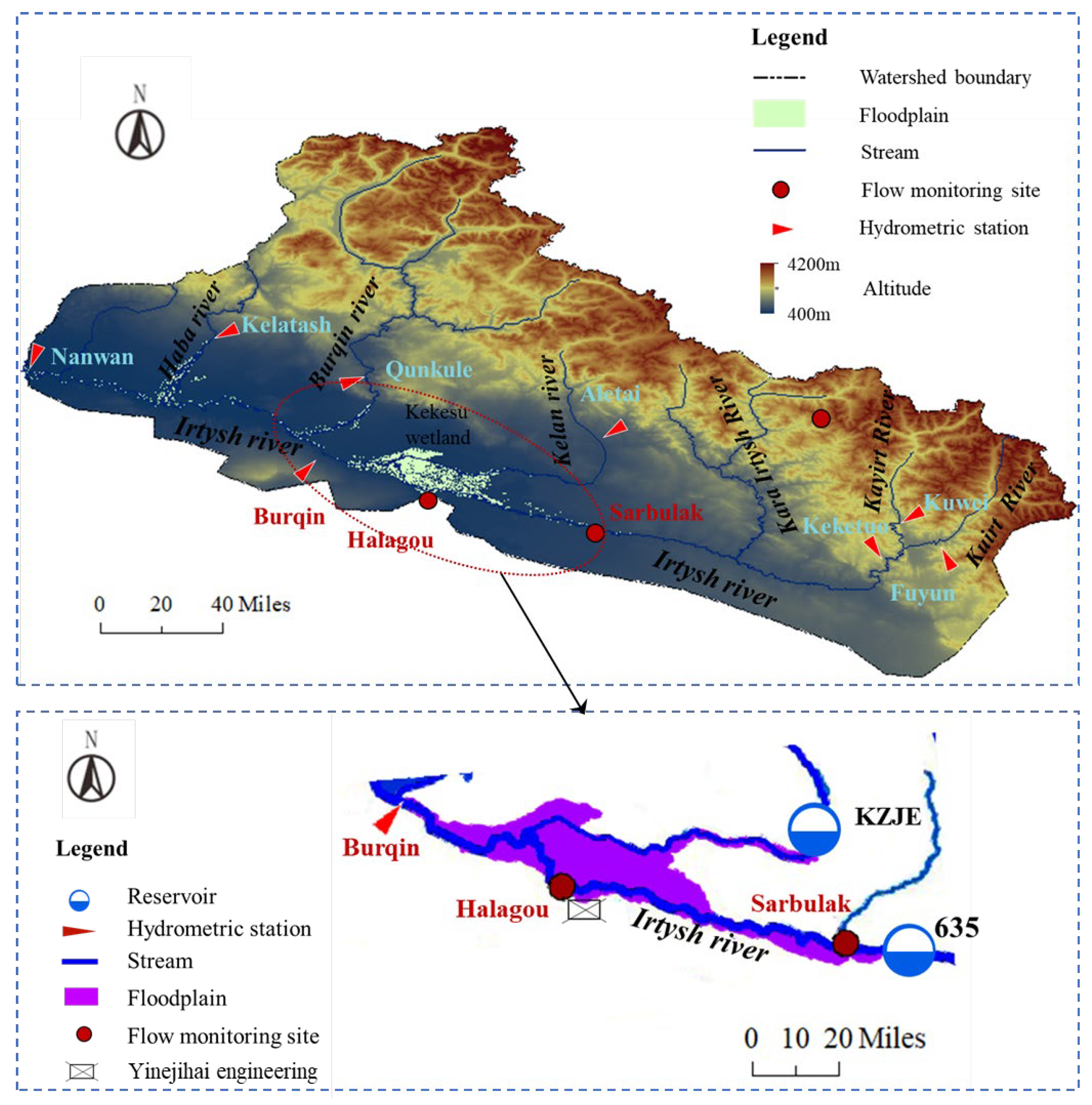
2. Site Description
3. Method
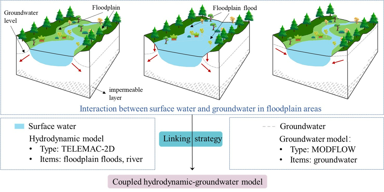
3.1. Hydrodynamic Model
3.1.1. Description of TELEMAC-2D Model
3.1.2. The Establishment of Hydrodynamic Model
3.2. GW Model
3.2.1. Description of MODFLOW Model
3.2.2. The Establishment of GW Model
- (1)
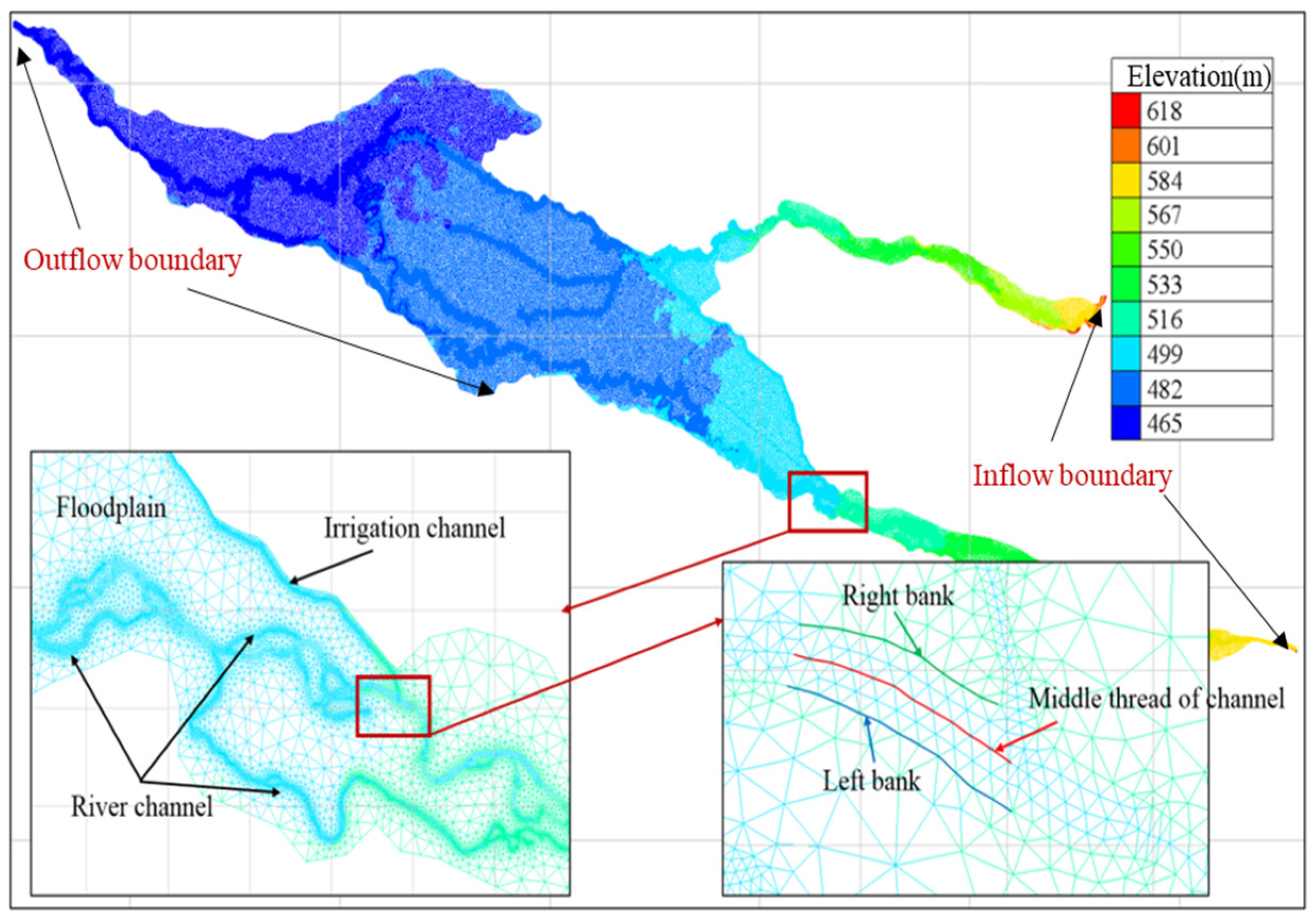
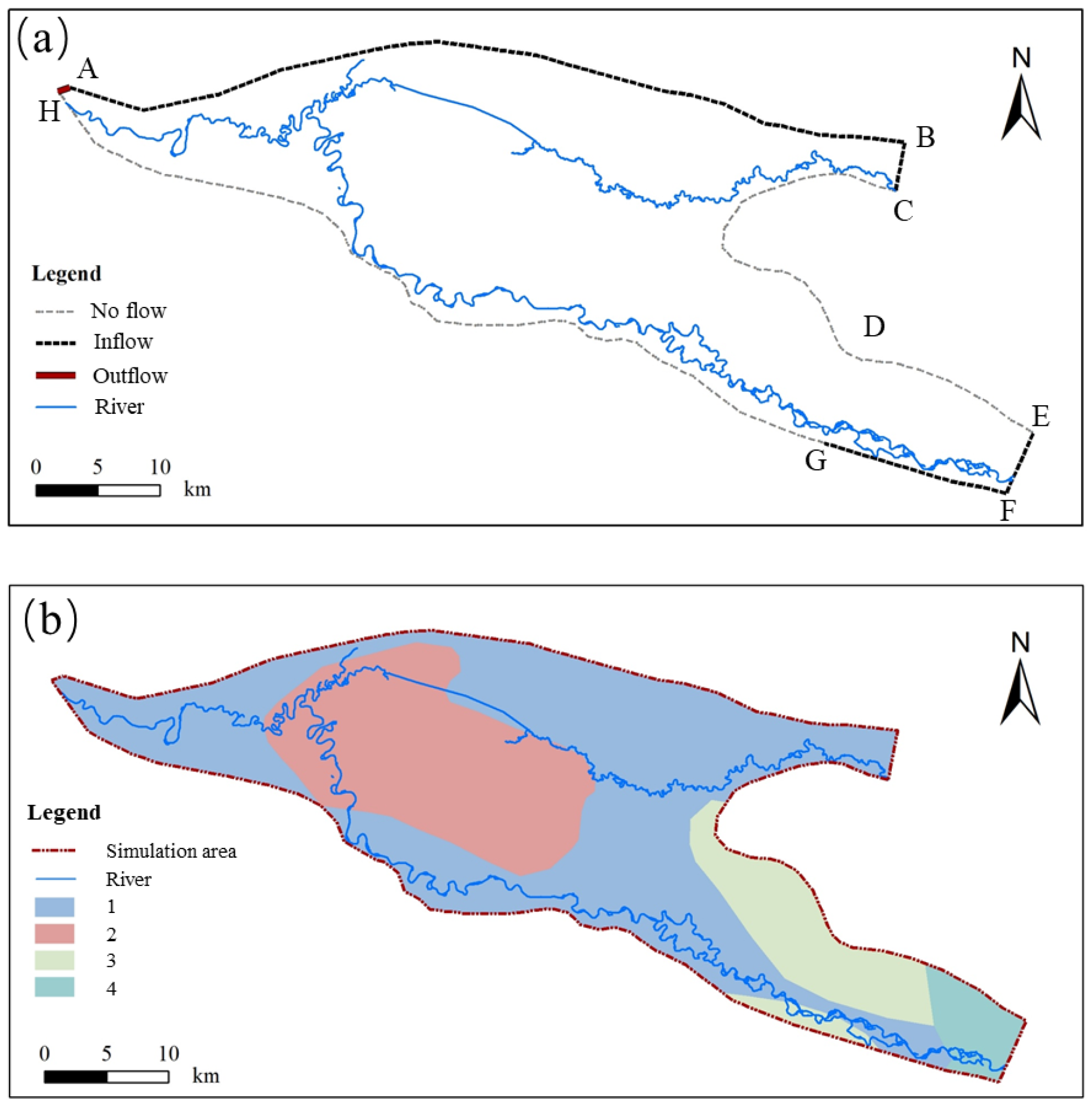
- The simulation range and model boundary conditions should be determined. In this study, the focus is on the floodplain area in the middle reaches of the Irtysh River, covering approximately 1104 km2. The lateral boundary conditions, which consider terrain, geology, and flow field data, encompass inflow boundaries, outflow boundaries, and zero flow (or water separation) boundaries, as shown in Figure 3a. Reasons for this determination are as follows: The BC section and the EF section are considered as lateral inflow sections of GW, and thus generalized as inflow boundaries. The ED section, perpendicular to the GW contour, is treated as an impermeable boundary due to the absence of water exchange. The CD section, with the presence of a mountain named the Small Bashaan Mountain on the eastern side, creating a distinct flow field, is treated as an impermeable boundary. The FG section is influenced by topography and the southern irrigation area, making it a lateral inflow boundary. The south of the HG section is a desert area, and the terrain is relatively flat, resulting in minimal water exchange, and therefore HG is generalized as a zero-flow boundary. The AH section is where GW exits, and is hence generalized as an outflow boundary. Finally, the AB section, influenced by the northern irrigation area, is treated as a lateral inflow boundary. The vertical boundary conditions consist of ground at the top and an impervious layer at the bottom.
- (2)
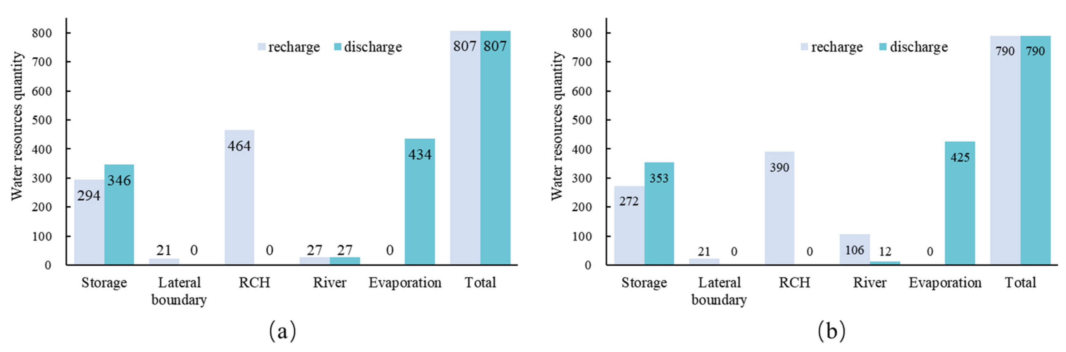
- The GW aquifer and source and sink terms should be correctly generalized. Based on the available hydrogeological data, the study area’s aquifers are characterized as homogeneous, isotropic single-layer unconfined aquifer. Considering the specific conditions, the GW model incorporates various recharge components, including floodplain flood GW recharge (FFGR), river channel seepage, canal system seepage, field irrigation infiltration, and lateral recharge. The method of obtaining FFGR will be discussed in the next section. River channel seepage is automatically calculated using the RIV package. Canal system seepage and field irrigation infiltration are calculated based on irrigation and canal data. Lateral recharge is computed using Darcy’s law formula, where hydraulic gradients are derived from GW contours. The main discharge components are represented by evapotranspiration, river channel discharge, and lateral GW discharge. Evaporation data are calculated by multiplying the evaporation coefficient (it has a value of 0.85 in this study) with the large water surface evaporation data from the meteorological station, and river channel discharge and lateral GW discharge are obtained using the same methods described above.
- (3)
- The model should be discretized in time and space.
- (4)
- The parameters should be determined.
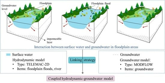
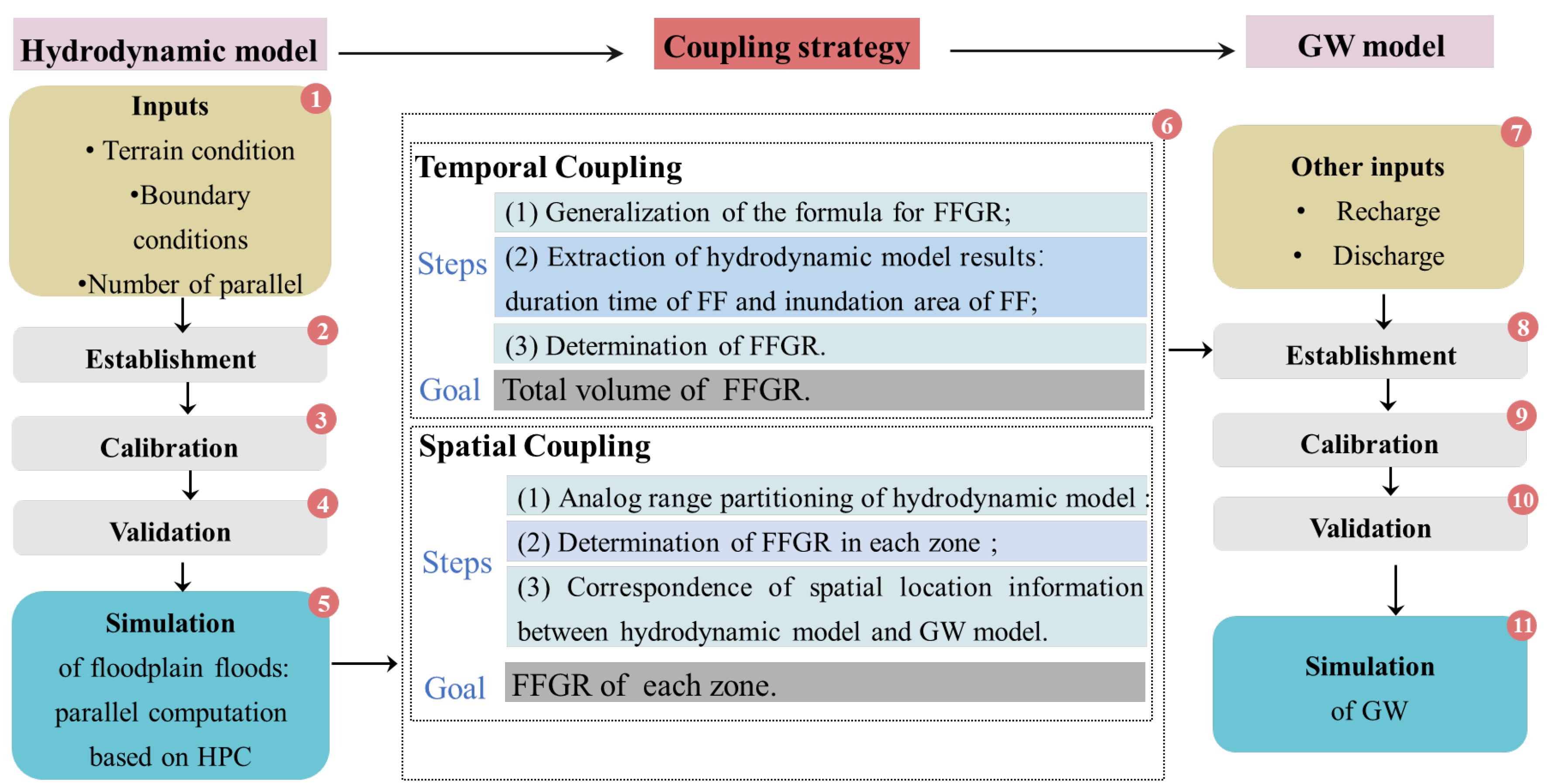
3.3. Hydrodynamic–GW Model Coupling Strategy
3.3.1. Temporal Coupling
- (1)
- Generalization of the formula for FFGR:
- (2)
- Extraction of hydrodynamic model results:
- (3)
- Determination of FFGR:
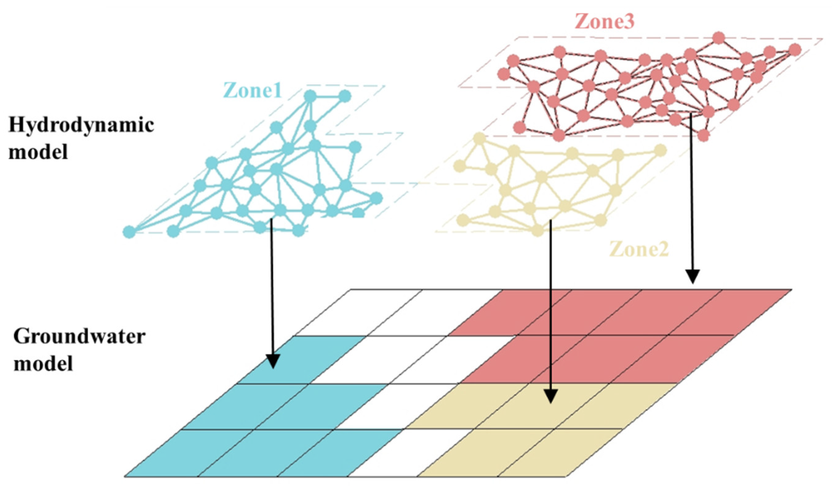
3.3.2. Spatial Coupling
- (1)
- Analog range partitioning of hydrodynamic model:
- (2)
- Determination of FFGR in each zone:
- (3)
- Correspondence of spatial location information:
4. Results
4.1. Calibration and Validation of the Models
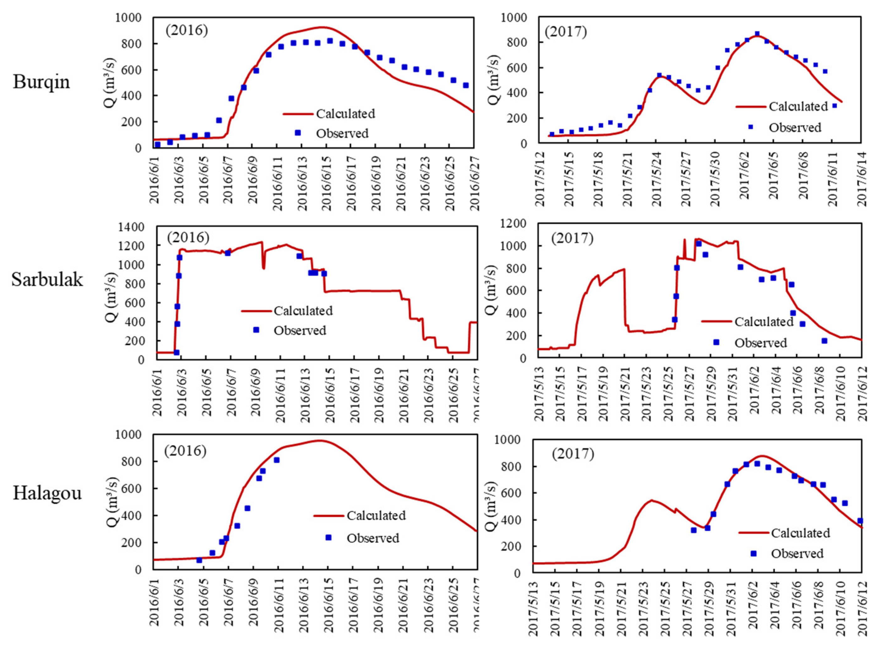
4.1.1. The 2D Hydrodynamic Model
4.1.2. The Coupled Hydrodynamic–GW Model
4.2. Water Balance of the Coupled SW–GW Model
5. Discussion
5.1. Accurate Spatiotemporal Simulation of GW Table
5.2. Recommendations during Coupled Model Modeling
- Digital Elevation Models (DEMs) are vital for both hydrodynamic and GW modeling, and it is crucial to carefully check and correct them to ensure accurate simulation results. The hydrodynamic model’s accuracy is directly influenced by precise elevation data, as it determines flow rates and directions. Similarly, the GW model relies on accurate elevation information to assess the deviation between the model’s top elevation and the phreatic level, known as the phreatic depth. To enhance simulation accuracy, it is recommended to utilize measured elevation data for both hydrodynamic and GW models.
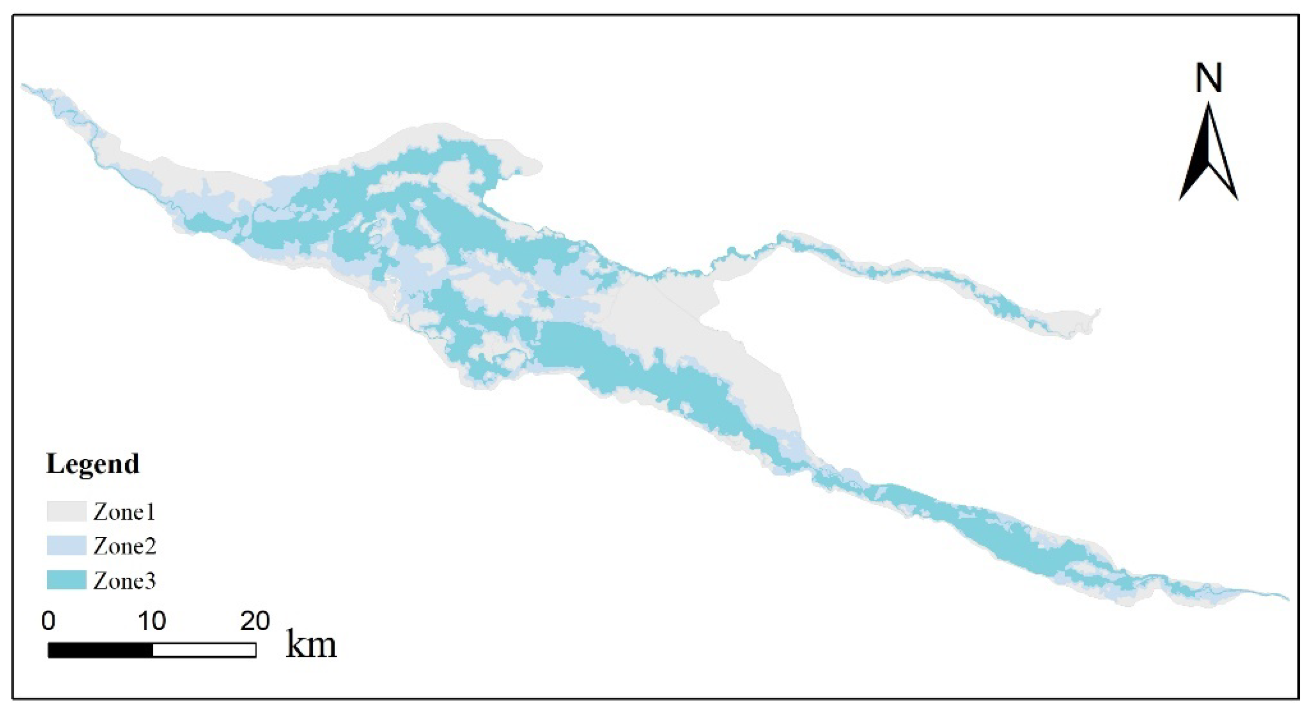
- Accurate zoning of the hydrodynamic model is crucial for the successful coupling strategy. In this study, the simulation range of the hydrodynamic model is divided into three zones based on the proportion of inundation time. The rationale behind this choice stems from the observation that finer partitioning based on the proportion of inundation time does not yield substantial differences in the resulting zone areas. However, pursuing a more refined partitioning approach would entail a significant increase in workload without commensurate benefits, rendering it cost ineffective. Therefore, it is recommended to determine the SW zoning based on the specific characteristics of the model.
5.3. Model Limitations
6. Conclusions
Author Contributions
Funding
Data Availability Statement
Acknowledgments
Conflicts of Interest
References
- Tockner, K.; Stanford, J.A. Riverine flood plains: Present state and future trends. Environ. Conserv. 2002, 29, 308–330. [Google Scholar] [CrossRef]
- Grizzetti, B.; Liquete, C.; Pistocchi, A.; Vigiak, O.; Zulian, G.; Bouraoui, F.; De Roo, A.; Cardoso, A.C. Relationship between Ecological Condition and Ecosystem Services in European Rivers, Lakes and Coastal Waters. Sci. Total Environ. 2019, 671, 452–465. [Google Scholar] [CrossRef]
- Gómez-Baggethun, E.; Tudor, M.; Doroftei, M.; Covaliov, S.; Năstase, A.; Onără, D.F.; Mierlă, M.; Marinov, M.; Doroșencu, A.C.; Lupu, G.; et al. Changes in Ecosystem Services from Wetland Loss and Restoration: An Ecosystem Assessment of the Danube Delta (1960–2010). Ecosyst. Serv. 2019, 39, 100965. [Google Scholar] [CrossRef]
- Karimi, S.S.; Saintilan, N.; Wen, L.; Valavi, R.; Cox, J. The ecohydrological impact of water resource developments through inundation regime analysis of a large semi-arid floodplain. J. Hydrol. 2021, 596, 126127. [Google Scholar] [CrossRef]
- Selwood, K.E.; Clarke, R.H.; McGeoch, M.A.; Mac Nally, R. Green Tongues into the Arid Zone: River Floodplains Extend the Distribution of Terrestrial Bird Species. Ecosystems 2016, 20, 745–756. [Google Scholar] [CrossRef]
- Ramberg, L.; Wolski, P.; Krah, M. Water balance and infiltration in a seasonal floodplain in the Okavango Delta, Botswana. Wetlands 2006, 26, 677–690. [Google Scholar] [CrossRef]
- Wu, C.; Webb, J.A.; Stewardson, M.J. Modelling Impacts of Environmental Water on Vegetation of a Semi-Arid Floodplain–Lakes System Using 30-Year Landsat Data. Remote Sens. 2022, 14, 708. [Google Scholar] [CrossRef]
- Sims, N.C.; Colloff, M.J. Remote sensing of vegetation responses to flooding of a semi-arid floodplain: Implications for monitoring ecological effects of environmental flows. Ecol. Indic. 2012, 18, 387–391. [Google Scholar] [CrossRef]
- Hayes, D.S.; Brändle, J.M.; Seliger, C.; Zeiringer, B.; Ferreira, T.; Schmutz, S. Advancing towards functional environmental flows for temperate floodplain rivers. Sci. Total Environ. 2018, 633, 1089–1104. [Google Scholar] [CrossRef]
- Best, J. Anthropogenic Stresses on the World’s Big Rivers. Nat. Geosci. 2018, 12, 7–21. [Google Scholar] [CrossRef]
- Chaparro, G.; O’Farrell, I.; Hein, T. Multi-scale analysis of functional plankton diversity in floodplain wetlands: Effects of river regulation. Sci. Total Environ. 2019, 667, 338–347. [Google Scholar] [CrossRef] [PubMed]
- Almeida, R.M.; Hamilton, S.K.; Rosi, E.J.; Barros, N.; Doria, C.R.C.; Flecker, A.S.; Fleischmann, A.S.; Reisinger, A.J.; Roland, F. Hydropeaking Operations of Two Run-of-River Mega-Dams Alter Downstream Hydrology of the Largest Amazon Tributary. Front. Environ. Sci. 2020, 8, 120. [Google Scholar] [CrossRef]
- Glenn, E.P.; Nagler, P.L.; Shafroth, P.B.; Jarchow, C.J. Effectiveness of environmental flows for riparian restoration in arid regions: A tale of four rivers. Ecol. Eng. 2017, 106, 695–703. [Google Scholar] [CrossRef]
- Hairan, M.H.; Jamil, N.R.; Looi, L.J.; Azmai, M.N.A. The assessment of environmental flow status in Southeast Asian Rivers: A review. J. Clean. Prod. 2021, 295, 126411. [Google Scholar] [CrossRef]
- Campbell, C.J.; Freestone, F.L.; Duncan, R.P.; Higgisson, W.; Healy, S.J. The more the merrier: Using environmental flows to improve floodplain vegetation condition. Mar. Freshw. Res. 2021, 72, 1185. [Google Scholar] [CrossRef]
- Nagler, P.L.; Barreto-Muñoz, A.; Borujeni, S.C.; Jarchow, C.J.; Gómez-Sapiens, M.M.; Nouri, H.; Herrmann, S.M.; Didan, K. Ecohydrological responses to surface flow across borders: Two decades of changes in vegetation greenness and water use in the riparian corridor of the Colorado River delta. Hydrol. Process. 2020, 34, 4851–4883. [Google Scholar] [CrossRef]
- Kendy, E.; Flessa, K.W.; Schlatter, K.J.; de la Parra, C.A.; Huerta, O.M.H.; Carrillo-Guerrero, Y.K.; Guillen, E. Leveraging environmental flows to reform water management policy: Lessons learned from the 2014 Colorado River Delta pulse flow. Ecol. Eng. 2017, 106, 683–694. [Google Scholar] [CrossRef]
- De Resende, A.F.; Schöngart, J.; Streher, A.S.; Ferreira-Ferreira, J.; Piedade, M.T.F.; Silva, T.S.F. Massive tree mortality from flood pulse disturbances in Amazonian floodplain forests: The collateral effects of hydropower production. Sci. Total Environ. 2019, 659, 587–598. [Google Scholar] [CrossRef]
- Larsen, S.; Karaus, U.; Claret, C.; Sporka, F.; Hamerlík, L.; Tockner, K. Flooding and hydrologic connectivity modulate community assembly in a dynamic river-floodplain ecosystem. PLoS ONE 2019, 14, e0213227. [Google Scholar] [CrossRef]
- Wise, W.R.; Annable, M.D.; Walser, J.A.E.; Switt, R.S.; Shaw, D.T. A Wetland- Aquifer Interaction Test. J. Hydrol. 1999, 227, 257–272. [Google Scholar] [CrossRef]
- Hunt, R.J.; Strand, M.; Walker, J.F. Measuring Groundwater-Surface Water Interaction and Its Effect on Wetland Stream Benthic Productivity, Trout Lake Watershed, Northern Wisconsin, USA. J. Hydrol. 2006, 320, 370–384. [Google Scholar] [CrossRef]
- Bye, J.A.; Narayan, K.A. Groundwater response to the tide in wetlands: Observations from the Gillman Marshes, South Australia. Estuar. Coast. Shelf Sci. 2009, 84, 219–226. [Google Scholar] [CrossRef]
- Parsons, D.F.; Hayashi, M.; van der Kamp, G. Infiltration and solute transport under a seasonal wetland: Bromide tracer experiments in Saskatoon, Canada. Hydrol. Process. 2004, 18, 2011–2027. [Google Scholar] [CrossRef]
- Bravo, H.R.; Jiang, F.; Hunt, R.J. Using groundwater temperature data to constrain parameter estimation in a groundwater flow model of a wetland system. Water Resour. Res. 2002, 38, 28-1–28-14. [Google Scholar] [CrossRef]
- Ladouche, B.; Weng, P. Hydrochemical assessment of the Rochefort marsh: Role of surface and groundwater in the hydrological functioning of the wetland. J. Hydrol. 2005, 314, 22–42. [Google Scholar] [CrossRef]
- Li, F.; Liu, Y.; Zhao, Y.; Deng, X.; Jiang, R. Regulation of shallow groundwater based on MODFLOW. Appl. Geogr. 2019, 110, 102049. [Google Scholar] [CrossRef]
- Ostad-Ali-Askari, K.; Kharazi, H.G.; Shayannejad, M.; Zareian, M.J. Effect of management strategies on reducing negative impacts of climate change on water resources of the Isfahan-Borkhar aquifer using MODFLOW. River Res. Appl. 2019, 35, 611–631. [Google Scholar] [CrossRef]
- Woldeamlak, S.T.; Batelaan, O.; De Smedt, F. Effects of climate change on the groundwater system in the Grote-Nete catchment, Belgium. Hydrogeol. J. 2007, 15, 891–901. [Google Scholar] [CrossRef]
- Guevara-Ochoa, C.; Medina-Sierra, A.; Vives, L. Spatio-temporal effect of climate change on water balance and interactions between groundwater and surface water in plains. Sci. Total Environ. 2020, 722, 137886. [Google Scholar] [CrossRef]
- Pryet, A.; Labarthe, B.; Saleh, F.; Akopian, M.; Flipo, N. Reporting of Stream-Aquifer Flow Distribution at the Regional Scale with a Distributed Process-Based Model. Water Resour. Manag. 2015, 29, 139–159. [Google Scholar] [CrossRef]
- Flipo, N.; Mouhri, A.; Labarthe, B.; Biancamaria, S.; Rivière, A.; Weill, P. Continental Hydrosystem Modelling: The Concept of Nested Stream–Aquifer Interfaces. Hydrol. Earth Syst. Sci. 2014, 18, 3121–3149. [Google Scholar] [CrossRef]
- Barthel, R.; Banzhaf, S. Groundwater and Surface Water Interaction at the Regional-scale—A Review with Focus on Regional Integrated Models. Water Resour. Manag. 2015, 30, 1–32. [Google Scholar] [CrossRef]
- Deb, P.; Kiem, A.S.; Willgoose, G. A linked surface water-groundwater modelling approach to more realistically simulate rainfall-runoff non-stationarity in semi-arid regions. J. Hydrol. 2019, 575, 273–291. [Google Scholar] [CrossRef]
- Akbari, F.; Shourian, M.; Moridi, A. Assessment of the climate change impacts on the watershed-scale optimal crop pattern using a surface-groundwater interaction hydro-agronomic model. Agric. Water Manag. 2022, 265, 107508. [Google Scholar] [CrossRef]
- Wei, X.; Bailey, R.T.; Records, R.M.; Wible, T.C.; Arabi, M. Comprehensive simulation of nitrate transport in coupled surface-subsurface hydrologic systems using the linked SWAT-MODFLOW-RT3D model. Environ. Model. Softw. 2019, 122, 104242. [Google Scholar] [CrossRef]
- Ehtiat, M.; Mousavi, S.J.; Srinivasan, R. Groundwater Modeling Under Variable Operating Conditions Using SWAT, MODFLOW and MT3DMS: A Catchment Scale Approach to Water Resources Management. Water Resour. Manag. 2018, 32, 1631–1649. [Google Scholar] [CrossRef]
- Aliyari, F.; Bailey, R.T.; Tasdighi, A.; Dozier, A.; Arabi, M.; Zeiler, K. Coupled SWAT-MODFLOW model for large-scale mixed agro-urban river basins. Environ. Model. Softw. 2019, 115, 200–210. [Google Scholar] [CrossRef]
- Alattar, M.H.; Troy, T.J.; Russo, T.A.; Boyce, S.E. Modeling the surface water and groundwater budgets of the US using MODFLOW-OWHM. Adv. Water Resour. 2020, 143, 103682. [Google Scholar] [CrossRef]
- Tian, Y.; Xiong, J.; He, X.; Pi, X.; Jiang, S.; Han, F.; Zheng, Y. Joint Operation of Surface Water and Groundwater Reservoirs to Address Water Conflicts in Arid Regions: An Integrated Modeling Study. Water 2018, 10, 1105. [Google Scholar] [CrossRef]
- Zhou, S.; Yuan, X.; Peng, S.; Yue, J.; Wang, X.; Liu, H.; Williams, D.D. Groundwater-surface water interactions in the hyporheic zone under climate change scenarios. Environ. Sci. Pollut. Res. 2014, 21, 13943–13955. [Google Scholar] [CrossRef]
- Joo, J.; Tian, Y.; Zheng, C.; Zheng, Y.; Sun, Z.; Zhang, A.; Chang, H. An Integrated Modeling Approach to Study the Surface Water-Groundwater Interactions and Influence of Temporal Damping Effects on the Hydrological Cycle in the Miho Catchment in South Korea. Water 2018, 10, 1529. [Google Scholar] [CrossRef]
- Sandu, M.-A.; Virsta, A. Applicability of MIKE SHE to Simulate Hydrology in Argesel River Catchment. Agric. Agric. Sci. Procedia 2015, 6, 517–524. [Google Scholar] [CrossRef]
- Sterte, E.J.; Johansson, E.; Sjöberg, Y.; Karlsen, R.H.; Laudon, H. Groundwater-Surface Water Interactions across Scales in a Boreal Landscape Investigated Using a Numerical Modelling Approach. J. Hydrol. 2018, 560, 184–201. [Google Scholar] [CrossRef]
- Boubacar, A.B.; Moussa, K.; Yalo, N.; Berg, S.J.; Erler, A.R.; Hwang, H.-T.; Khader, O.; Sudicky, E.A. Characterization of groundwater –surface water interactions using high resolution integrated 3D hydrological model in semiarid urban watershed of Niamey, Niger. J. Afr. Earth Sci. 2020, 162, 1. [Google Scholar] [CrossRef]
- Salem, A.; Dezső, J.; El-Rawy, M.; Lóczy, D. Hydrological Modeling to Assess the Efficiency of Groundwater Replenishment through Natural Reservoirs in the Hungarian Drava River Floodplain. Water 2020, 12, 250. [Google Scholar] [CrossRef]
- Vrzel, J.; Ludwig, R.; Gampe, D.; Ogrinc, N. Hydrological system behaviour of an alluvial aquifer under climate change. Sci. Total Environ. 2019, 649, 1179–1188. [Google Scholar] [CrossRef]
- Werner, A.D.; Gallagher, M.R.; Weeks, S.W. Regional-Scale, Fully Coupled Modelling of Stream–Aquifer Interaction in a Tropical Catchment. J. Hydrol. 2006, 328, 497–510. [Google Scholar] [CrossRef]
- Ntona, M.M.; Busico, G.; Mastrocicco, M.; Kazakis, N. Modeling groundwater and surface water interaction: An overview of current status and future challenges. Sci. Total Environ. 2022, 846, 157355. [Google Scholar] [CrossRef]
- Li, Y.; Yao, J.; Tan, Z.; Zhang, Q. Advances in Surface Water-Groundwater Interactions in Floodplain Wetlands. J. China Hydrol. 2019, 39, 14–21. [Google Scholar]
- Reisenbüchler, M.; Bui, M.D.; Skublics, D.; Rutschmann, P. An integrated approach for investigating the correlation between floods and river morphology: A case study of the Saalach River, Germany. Sci. Total Environ. 2019, 647, 814–826. [Google Scholar] [CrossRef]
- Hervouet, J. Hydrodynamics of Free Surface Flows: Modelling with the Finite Element Method; John Wiley & Sons: Chichester, UK, 2007; pp. 83–133. [Google Scholar]
- Wang, D.; Zhang, S.; Wang, G.; Liu, Y.; Wang, H.; Gu, J. Reservoir Regulation for Ecological Protection and Remediation: A Case Study of the Irtysh River Basin, China. Int. J. Environ. Res. Public Health 2022, 19, 11582. [Google Scholar] [CrossRef] [PubMed]
- Yang, H.; Rahardjo, H.; Leong, E.-C. Behavior of Unsaturated Layered Soil Columns during Infiltration. J. Hydrol. Eng. 2006, 11, 329–337. [Google Scholar] [CrossRef]
- Ochoa, C.G.; Sierra, A.M.; Vives, L.; Zimmermann, E.; Bailey, R. Spatio-temporal patterns of the interaction between groundwater and surface water in plains. Hydrol. Process. 2020, 34, 1371–1392. [Google Scholar] [CrossRef]
- Hu, L.; Xu, Z.; Huang, W. Development of a river-groundwater interaction model and its application to a catchment in Northwestern China. J. Hydrol. 2016, 543, 483–500. [Google Scholar] [CrossRef]
- Kumbier, K.; Rogers, K.; Hughes, M.G.; Lal, K.K.; Mogensen, L.A.; Woodroffe, C.D. An Eco-Morphodynamic Modelling Approach to Estuarine Hydrodynamics & Wetlands in Response to Sea-Level Rise. Front. Mar. Sci. 2022, 9, 613. [Google Scholar] [CrossRef]
- Haverson, D.; Bacon, J.; Smith, H.C.; Venugopal, V.; Xiao, Q. Modelling the hydrodynamic and morphological impacts of a tidal stream development in Ramsey Sound. Renew. Energy 2018, 126, 876–887. [Google Scholar] [CrossRef]
- Stark, J.; Plancke, Y.; Ides, S.; Meire, P.; Temmerman, S. Coastal flood protection by a combined nature-based and engineering approach: Modeling the effects of marsh geometry and surrounding dikes. Estuar. Coast. Shelf Sci. 2016, 175, 34–45. [Google Scholar] [CrossRef]
- Moulinec, C.; Denis, C.; Pham, C.T.; Rougé, D.; Hervouet, J.M.; Razafindrakoto, E.; Barber, R.W.; Emerson, D.R.; Gu, X.J. Telemac: An Efficient Hydrodynamics Suite for Massively Parallel Architectures. Comput. Fluids 2011, 51, 30–34. [Google Scholar] [CrossRef]
- Fu, Y.; Dong, Y.; Xie, Y.; Xu, Z.; Wang, L. Impacts of Regional Groundwater Flow and River Fluctuation on Floodplain Wetlands in the Middle Reach of the Yellow River. Water 2020, 12, 1922. [Google Scholar] [CrossRef]
- Hester, E.T.; Guth, C.R.; Scott, D.T.; Jones, C.N. Vertical surface water–groundwater exchange processes within a headwater floodplain induced by experimental floods. Hydrol. Process. 2016, 30, 3770–3787. [Google Scholar] [CrossRef]
- Zhu, X.; Wu, J.; Nie, H.; Guo, F.; Wu, J.; Chen, K.; Liao, P.; Xu, H.; Zeng, X. Quantitative assessment of the impact of an inter-basin surface-water transfer project on the groundwater flow and groundwater-dependent eco-environment in an oasis in arid northwestern China. Hydrogeol. J. 2018, 26, 1475–1485. [Google Scholar] [CrossRef]
- Qi, Q.Q.; Xu, Y.X.; Song, S.H.; Zhang, Z.Z. Application of a Groundwater Modelling System in Groundwater Environmental Impact Assessment of River and Lake Connection in Western Jilin Region. Appl. Ecol. Environ. Res. 2019, 17, 5059–5066. [Google Scholar] [CrossRef]
- Vernoux, J.F.; Horriche, F.J.; Ghoudi, R. Numerical groundwater flow modeling for managing the Gabes Jeffara aquifer system (Tunisia) in relation with oasis ecosystems. Hydrogeol. J. 2020, 28, 1077–1090. [Google Scholar] [CrossRef]
- Khan, H.F.; Yang, Y.C.E.; Ringler, C.; Wi, S.; Cheema, M.J.M.; Basharat, M. Guiding Groundwater Policy in the Indus Basin of Pakistan Using a Physically Based Groundwater Model. J. Water Resour. Plan. Manag. 2017, 143, 05016014. [Google Scholar] [CrossRef]


| Data Type | Data Content | Effect | Source |
|---|---|---|---|
| Geological data | Channel section, 2.5 m contour line, measured elevation points with a precision of 1 km | Generating the simulation area and terrain file | Geological survey results of the study area |
| DEM data with a resolution of 15 m | Generating the simulation area and terrain file | Bigemap | |
| Hydrological data | 2 h outflow processes of the 635 and KZJE reservoirs | Inflow boundary | Reservoir operation and scheduling data |
| Daily flows of Yinejihai engineering | Outflow boundary | Operation and scheduling data of Yinejihai engineering | |
| Daily water flows of the Burqin Hydrological Station | Calibration and validation | Burqin hydrometric station | |
| Daily water levels of the Burqin Hydrological Station | Outflow boundary | Burqin hydrometric station | |
| Daily water flows of Sarbulak, and Halagou Mudao Bridge | Calibration and validation | On-site monitoring data | |
| Meteorological data | Daily evaporation | Water loss calculation | Aletai hydrometric station |
| Infiltration observation data | Water loss calculation | Field data | |
| Remote sensing image data | Remote sensing imaging from the SPOT-6 satellite and Environment-1 satellite | Generating the simulation area and terrain file | Bigemap |
| Data Type | Data Content | Effect | Source |
|---|---|---|---|
| Topographic geological data | Elevation data obtained from surveyed points with an accuracy of 1 km, Hydrogeological cross-section, soil properties, contour map of GW level | Model establishment | Geological survey results of the study area |
| The DEM data with a resolution of 15 m | Model establishment | Bigemap | |
| Recharge and discharge items | Daily evaporation | Model establishment | Burqin and Aletai hydrometric station |
| Irrigation area and monthly amount of irrigation | Model establishment | Regional agricultural statistics annual report | |
| Other | Measured data of GW level on the 10th, 20th, and 30th day of each month | Model calibration and validation | Field measurement data |
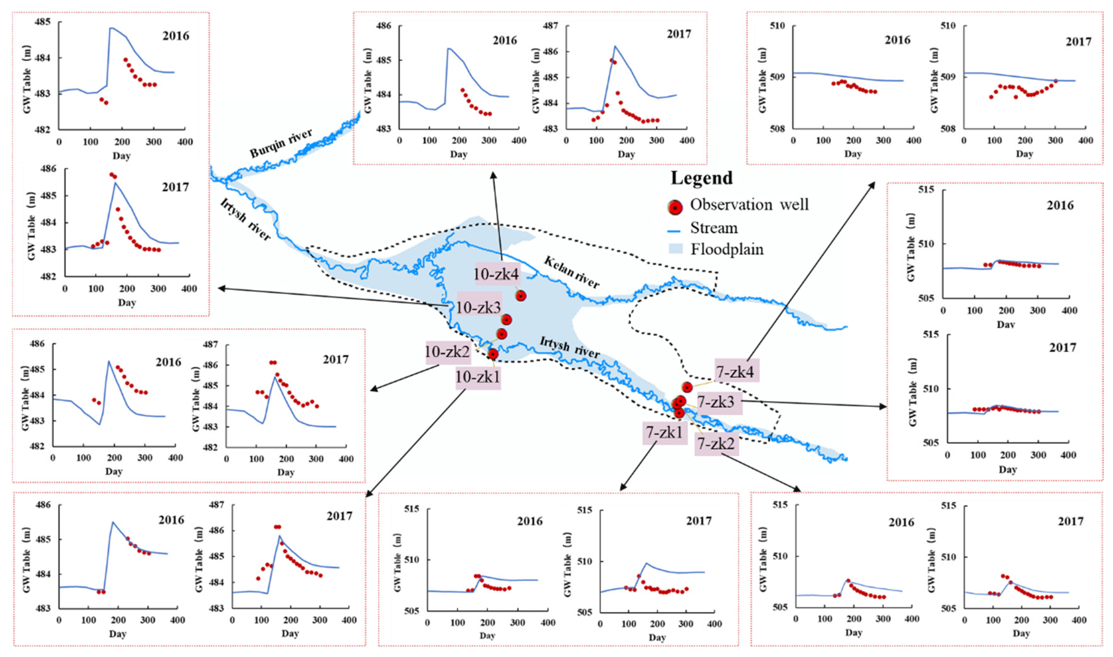
| Observation Well | 7-zk1 | 7-zk2 | 7-zk3 | 7-zk4 | 10-zk1 | 10-zk2 | 10-zk3 | 10-zk4 | Mean Value |
|---|---|---|---|---|---|---|---|---|---|
| 2016 | 0.79 | 0.63 | 0.25 | 0.18 | 0.05 | 0.88 | 0.55 | 0.74 | 0.51 |
| 2017 | 1.74 | 0.56 | 0.2 | 0.27 | 0.49 | 0.94 | 0.75 | 1.24 | 0.77 |
Disclaimer/Publisher’s Note: The statements, opinions and data contained in all publications are solely those of the individual author(s) and contributor(s) and not of MDPI and/or the editor(s). MDPI and/or the editor(s) disclaim responsibility for any injury to people or property resulting from any ideas, methods, instructions or products referred to in the content. |
© 2023 by the authors. Licensee MDPI, Basel, Switzerland. This article is an open access article distributed under the terms and conditions of the Creative Commons Attribution (CC BY) license (https://creativecommons.org/licenses/by/4.0/).
Share and Cite
Liu, Y.; Jiang, Y.; Zhang, S.; Wang, D.; Chen, H. Application of a Linked Hydrodynamic–Groundwater Model for Accurate Groundwater Simulation in Floodplain Areas: A Case Study of Irtysh River, China. Water 2023, 15, 3059. https://doi.org/10.3390/w15173059
Liu Y, Jiang Y, Zhang S, Wang D, Chen H. Application of a Linked Hydrodynamic–Groundwater Model for Accurate Groundwater Simulation in Floodplain Areas: A Case Study of Irtysh River, China. Water. 2023; 15(17):3059. https://doi.org/10.3390/w15173059
Chicago/Turabian StyleLiu, Yin, Yunzhong Jiang, Shuanghu Zhang, Dan Wang, and Huan Chen. 2023. "Application of a Linked Hydrodynamic–Groundwater Model for Accurate Groundwater Simulation in Floodplain Areas: A Case Study of Irtysh River, China" Water 15, no. 17: 3059. https://doi.org/10.3390/w15173059
APA StyleLiu, Y., Jiang, Y., Zhang, S., Wang, D., & Chen, H. (2023). Application of a Linked Hydrodynamic–Groundwater Model for Accurate Groundwater Simulation in Floodplain Areas: A Case Study of Irtysh River, China. Water, 15(17), 3059. https://doi.org/10.3390/w15173059