Article

An Analytical Model Coupled with Orthogonal Experimental Design Is Used to Analyze the Main Controlling Factors of Multi-Layer Commingled Gas Reservoirs

1
State Key Laboratory of Shale Oil and Gas Enrichment Mechanisms and Effective Development, SINOPEC, Beijing 100083, China
2
Sinopec Key Laboratory of Shale Oil/Gas Exploration and Production Technology, SINOPEC, Beijing 100728, China
3
School of Earth Resources, China University of Geosciences, Wuhan 430074, China
*
Author to whom correspondence should be addressed.
Water 2023, 15(17), 3052; https://doi.org/10.3390/w15173052
Submission received: 20 July 2023 / Revised: 18 August 2023 / Accepted: 21 August 2023 / Published: 25 August 2023
(This article belongs to the Special Issue Fluid Dynamics Modeling in Porous Media)

Abstract

:
The majority of China’s multi-layer low permeability tight gas reservoirs are currently being extracted through the method of multi-layer co-production. However, due to the significant disparity in physical properties and varying degrees of pressure depletion among the production layers, elucidating the primary factors influencing the productivity contribution of each gas layer remains challenging. A multi-factor analytical model is proposed for commingled gas wells with multiple layers. An unstable model is established for the production of commingled layers, and the problem of flow distribution is addressed using the Duhamel convolution principle. The Laplace transform is subsequently employed to derive the solution in the Laplace domain, which can be inverted utilizing the Stehfest inversion algorithm to obtain a real-time domain solution. The influence of reservoir factors on the stratification contribution rate has been comprehensively analyzed, encompassing permeability, porosity, initial pressure, drainage radius, and layer thickness. The orthogonal test design was employed to conduct range analysis and variance analysis separately, yielding the primary and secondary order as well as influence weight of the five factors. The findings demonstrate that, within this gas reservoir, the discharge radius, thickness, and porosity are identified as the primary factors influencing gas well productivity. Furthermore, seven horizontal flow charts illustrating the double-layer gas reservoir and five horizontal flow charts depicting single-factor variations in the double-layer gas reservoir were constructed. These charts provide a clear visualization of the impact of each reservoir factor on stratification’s contribution rate. In contrast to previous studies, this novel approach presents a comprehensive optimization framework that ranks the influence weights of individual factors and identifies the most significant factors impacting multi-layer gas reservoirs. The presented method also serves as a foundation for the subsequent selection of multi-layer gas reservoirs, formulation of gas well stimulation measures, and efficient development.

1. Introduction

Due to the formation of sedimentary layers in various geological ages, many reservoirs exhibit multiple layer characteristics. The permeability and porosity vary across these layers, which can either be connected or disconnected. In cases where there is strong inter-layer leakage flow and good inter-layer connectivity, the dynamic characteristics resemble those observed in a single-layer scenario. However, if the layers are only connected through the wellbore, they clearly demonstrate multi-layer characteristics [1].
The characteristics are significantly different between multi-layer gas reservoirs and single-layer gas reservoirs. This is evident in the disparate depletion rates observed across each production layer, leading to variations in pressure and occurrences of interlayer channeling as well as wellbore backflow [2]. To meet production requirements, many production wells employ a multi-layer combined production approach. During production, the output of multi-layer commingled wells may occasionally be lower than the sum of individual layer outputs, which contradicts expectations and often perplexes reservoir engineers in the field. Investigating seepage characteristics and productivity factors of layered reservoirs is essential for practical analysis and interpretation of multi-layer commingled gas wells, guiding the selection of appropriate production pressure differentials, and facilitating development of multi-layer gas fields.
The investigation of unstable seepage flow in multi-layer commingled mining has been conducted since the 1960s, with numerous valuable studies undertaken by esteemed scholars [3,4,5]. Lefkovits et al. pioneered the application of analytical methods to investigate a multi-layer system model devoid of interlayer fouling, obtaining solutions for bottomhole pressure and production in a circular closed reservoir with an arbitrary number of layers, and conducting a comprehensive analyzing specifically focusing on the two-layer case. While the study holds significant importance, its practical utility is constrained by its failure to consider inter-layer crossflow. Russell and Prats conducted a comprehensive investigation on the multi-layer system model with crossflow, resulting in a novel solution for fixed bottom hole pressure, effectively addressing the limitations of previous research. The study conclusively demonstrated that inter-layer crossflow significantly influences the dynamic response of pressure during the transition stage from no crossflow to a single-layer homogeneous response. Additionally, scholars have extensively explored diverse initial pressure, boundary, porosity, and permeability conditions by integrating them into various models for further examination [6,7,8]. Papadopulos successfully resolved the issue of disparate pressures and pressure distributions across layers by obtaining an exact solution for a two-layer homogeneous and infinitely bounded aquifer model. Kucuk et al. developed an analytical solution applicable to scenarios involving distinct initial pressures and external boundary conditions in each layer, including complex cases featuring partial perforation, fractured wells, dual media, and external boundary conditions.
The aforementioned scholars overlooked the inclusion of the wellbore storage coefficient and skin factor in the study. However, as research progressed, it became evident to many scholars that incorporating these factors into the model is crucial, leading to numerous subsequent investigations [9,10,11,12,13]. Tariq et al. expanded the well-testing model for a multi-layer non-channeling flow system, incorporating both the effects of the wellbore storage effect and skin factor. Larson addressed the challenge of multi-layer commingled production with varying initial conditions, but it was assumed to be under constant rate conditions in the wellbore, and there still exist challenges in dealing with the problem of wellbore storage. Bourdet proposed a two-layer channeling reservoir model that incorporates the effects of the wellbore storage and skin effect. In the subsequent year, Mavor utilized a combinatorial technique to consider the influence of the wellbore storage effect, and applied the concept of parallel resistance to solve the multi-layer connected reservoir model. Rahman and Mattarm introduced a new analytical model that accounts for both the skin factor and wellbore storage effects in order to address instantaneous flow problems associated with commingled production in tight gas reservoirs featuring different initial pressures. This model is suitable for handling variations in production steps before and during production and construction stages, as well as constant pressure or non-flow conditions at the outer boundary of each layer.
Additionally, researchers have studied the calculation model for flow in each layer under varying pressure factors and obtained a series of results during this process [14,15]. Several scholars have utilized the relationship between flow rate at a constant pressure and pressure at a constant flow rate [14,16,17,18]. By considering the fundamental condition that the flow rates of individual layers are independent from each other during constant pressure production, the respective layer’s flow rate is determined, followed by determining the wellbore pressure. Milad et al. established a hydraulic coupling parameter model for multi-layer shale gas reservoirs using an effective iterative numerical simulation method to couple wellbore and gas reservoirs. A methodology is proposed for modeling and simulating commingled production from multiple shale-gas layers while accounting for changes in both pressure and flow within each layer.
Many scholars have conducted extensive research on production performance and prediction models in order to enhance the utilization of multi-layer commingled production technology for high-efficiency development in practical production. Ei-Banbi and Robert developed a stratified steady flow model for multi-layer commingled production data of tight gas reservoirs by combining the material balance equation with the gas steady flow equation [19]. This approach enables analysis and prediction of production performance for multi-layer commingled production, obtaining geological reserves of natural gas (OGIP) for each layer in tight gas reservoirs and evaluating the relative importance of each layer. Building upon Ei-Banbi and Rober’s established multi-layer commingled production model, Arevalo-Villagran improved the productivity prediction method for multi-layer commingled gas wells by further incorporating the actual boundary flow equation into the material balance equation, thereby proposing a novel multi-layer commingled production model capable of matching and predicting production outcomes [20]. This model can be used to calculate natural gas geological reserves, productivity index, and production rate of each layer while also enabling predictions regarding the individual layer’s future output.
As widely recognized, the analysis of the interlayer interference mechanism in multi-layer commingled production systems has been a focal point of research on multi-layer commingled production models for decades. Over the course of several decades, numerous scholars have conducted studies on this issue utilizing numerical simulations and other methods, resulting in a series of valuable findings. After analyzing the main factors contributing to interlayer interference, Zhang et al. concluded that they believed multi-layer commingled mining and differences in pressure systems were conditions for such interferences to occur [21]. Wang et al. [22,23] developed a methodology to calculating the interlayer interference coefficient of gas wells based on the binomial productivity formula and wellbore pressure calculation model derived from a physical model of multi-layer commingled production. Over the past decade, numerous scholars have extensively investigated the factors influencing interlayer interference in multi-layer commingled mining through the establishment of diverse mathematical and physical models, as well as utilizing numerical simulations, laboratory tests, and other methodologies. According to variations in research methodologies, the analysis can be categorized into three main approaches: (1) Through the establishment of a two-layer model without crossflow between layers, a physical model of multi-layer commingled production in gas wells, a rate transient analysis (RTA) and a structured RTA model of gas wells, a steady-state two-phase pipe flow model, and a radial multi-layer commingled production numerical model [24,25,26,27,28], the factors influencing interlayer interference were analyzed, and it was determined that the main factors affecting interlayer interference were interlayer pressure difference, reservoir physical properties, and interlayer span. Furthermore, the impact of each layer’s properties on multi-layer commingled production was evaluated, including permeability, porosity, thickness, initial pressure, and compressibility. (2) By conducting a visible multi-tube water flooding experiment, Huang et al. successfully quantified the interlayer interference in the multi-layer commingled production of offshore heavy oil reservoirs and established a theoretical model to predict directional well productivity [29]. (3) Zhao et al. employed the grey lattice Boltzmann method to evaluate how permeability and pressure differences affect interlayer interference in multi-layer commingled production [30]. It can be inferred that the interlayer interference coefficient exhibits a linear increase with the rise in pressure differential during multi-layer commingled production of gas reservoirs. Moreover, reservoirs with lower permeability exhibit more pronounced levels of interference.
In recent years, conventional oil production has remained stable, while advancements in the oil industry have significantly boosted unconventional oil production. Compared to conventional oil and gas reservoirs, unconventional oil and gas reservoirs exhibit a more intricate geological structure. Therefore, it is imperative to consider various factors such as reservoir density and heterogeneity when investigating the seepage behavior of these reservoirs. By incorporating the dynamic characteristics of three distinct pore systems, namely inorganic matter, organic matter, and natural fractures, Yan et al. [31] have successfully developed a micro-scale multi-pore model for fluid flow in shale reservoirs. This advancement not only enhances our understanding of the intricate flow mechanism but also paves the way for its potential extension to the reservoir scale through technological advancements. In order to investigate the flow mechanism in the re-reservoir of tight oil reservoirs, Wang and Yan et al. [32,33] conducted a series of studies on modeling the composition of tight oil. They proposed a comprehensive model for tight oil reservoir composition that incorporates the influence of nanopores. This model accurately simulates the rock and fluid characteristics affected by nanopores, resolves inconsistencies in the gas–oil ratio (GOR), significantly simplifies history matching procedures, and enhances recovery prediction reliability.
Numerical simulation methods are crucial for studying oil and gas reservoir seepage behavior. In the past decade, researchers have focused on enhancing these methods through novel algorithms. Tarip, Xu, Gudala et al. [34,35,36,37,38] have made significant advancements using the integrating inversion neural network (INN), particle swarm optimization evolutionary algorithm (PSO), and deep learning (DL) models to investigate reservoir seepage mechanisms and management frameworks. This represents a recent research breakthrough that requires further exploration to provide a more comprehensive description of reservoir characteristics.
In summary, the analysis of interlayer interference mechanism and influencing factors in a multi-layer commingled gas reservoir is typically done through three methods: indoor experiments, numerical simulations, and production model establishment. However, these methods have some drawbacks such as high costs for laboratory experiment simulation and a lack of parameters in production models or quantitative characterization in some approaches. The present paper proposes a novel mathematical model for multi-layer commingled production taking into account multiple influencing factors. By integrating the unstable seepage model of multi-layer commingled production with orthogonal experimental design, a comprehensive analysis is conducted on the proportion of each control factor affecting the productivity of commingled gas reservoirs, leading to a profound understanding of the unique seepage behavior in such reservoirs. In comparison with previous research, this model considers the influence of multiple factors on productivity and employs orthogonal testing to rank their importance in relation to multi-layer gas reservoirs. This provides a foundation of gas well stimulation measures, and efficient development practices for multi-layer gas reservoirs.
The following provides a concise overview of this paper. In Section 2, the governing equations and analytical solutions of the unstable seepage model of multi-layer commingled production are presented. Section 3 conducts an analysis on the combination of orthogonal test design, determining both the primary and secondary order of each influencing factor as well as their respective influence weights. Finally, in Section 4, conclusive remarks are provided.

2. Mathematical Model

2.1. Establishment of Constant Production Mathematical Model

Figure 1 depicts the schematic diagram of a physical model for multi-layer combined gas production. In this model, it is assumed that there exists a combined gas production well at the center of a closed gas reservoir with initial pressure pij, permeability kj, porosity φj, thickness hj, and drainage radius rej maintained at constant production rate. Under the general modeling condition, the governing equation for micro-compressible fluids is established:
2 Δ p p j r 2 + 1 r Δ p p j r = η j Δ p p j t ,   η j = k h j ϕ μ c t h j ,   Δ p p j = p p j i p p j , j = 1 , 2 , , n
Initial conditions:
Δ p p j r , 0 = 0
Outer boundary conditions:
Δ p p j r e j , t r = k f d j Δ p p j k j r e j ln r f d j / r e j
Inner boundary conditions:
p p j r w , t = p p j s t
r Δ p p j s r r = r w = q j s c t μ g B g i 2 π k h j
j = 1 n q j s c t = q s c
where pji—original formation pressure for layer j, MPa; ppj—gas pseudo pressure for layer j, MPa; φj—porosity for layer j; kj—permeability for layer j, μm2; kfdj—recharge permeability for layer j, μm2; hj—thickness for layer j, m; ctj—comprehensive compression coefficient for layer j, 1/MPa; rej—drainage radius for layer j, m; rfd—drainage radius for layer j, m; r—wellbore radius, m; pjs(t)—bottomhole pressure, MPa; qjsc(t)—surface production for layer j, m3/D; and qsc—surface production of a gas well, m3/D.

2.2. Laplace Solution of Constant Production Equation

The variable flow problem is summarized for the aforementioned Equations (1)–(6). In accordance with the Duhamel superposition principle, the following relations are established for the jth layer:
p p j s t = p p j i B g i t 0 t q j s c τ p p j r s t τ d τ
where ppjsr represents the solution to the problem subject to dimensionless flow per unit conditions. Upon applying dimensionless and Laplace transform, we obtain:
p ˜ p j s D ( r D , s ) = 1 s p p j i D + q ˜ j s c D ( s ) s p ˜ p j r s D ( r D , s )
If the dimensionless flow of a single layer is all 1, that is, qJd = 1, the solution of the pull-space pressure under fixed production can be obtained through Laplace transform as follows:
p ˜ p j s r D ( r D , s ) = 1 s κ j s z j K 0 ( r D s z j ) + C j λ I 0 ( r D s z j ) K 1 ( s z j ) C j λ I 1 ( s z j ) ,   z j = ω j / κ j
In the formula:
C j λ = r j e D s z j K 1 ( r j e D s z j ) + λ j K 0 ( r j e D s z j ) r j e D s z j I 1 ( r j e D s z j ) λ j I 0 ( r j e D s z j ) ,   λ j = k f d j k j r e j D ln r f d j / r e j
In the case of a closed boundary, λj = 0, while for a constant pressure boundary, λj → ∞. I0(v) and I1(v) are the first class of deformed Bessel functions, whereas K0(v) and K1(v) belong to the second class of deformed Bessel functions. The calculation of single-layer liquid production qjD(tD) can be performed using Formula (8).

2.3. Real-Time Domain Solution of Constant Production Problem

Define the average pressure as:
p p j a v g t = 1 V j T V w V j T p p j r , t d V
where VjT—total volume of discharge area, m3 and Vw—discharge shaft volume, m3.
Then, for the plane radial flow case:
p p j a v g t = 1 r e 2 r w 2 r w r j e r p p j s r , t d r
Substitute Formula (8) into Formula (13) after Laplace transformation to obtain:
p ˜ p j a v g D s = 2 r e D 2 1 1 r j e D r D 1 s p p j i D + q ˜ j s c D s s p ˜ p j r s D r D , s d r D   = 1 s p p j i D + 2 s q ˜ j s c D s r e D 2 1 1 r j e D r D p ˜ p j r s D r D , s d r D
Substitute Formula (9) into the above formula and invert by Stehfest to obtain the real-time domain solution of the average pressure:
p p j a v g D t D = p p j i D + τ j ω j 2 r j e D 2 1 0 t D q j s c D τ d τ
After dimensionalization, it can be obtained:
p p j i p p j a v g t = 0.092 r j e 2 r w 2 T j φ c t h j μ i 0 t q j s c τ d τ
where the left side of the equation represents the average pseudo pressure drop in layer j, while the right side is the cumulative production.

3. Results and Discussion

3.1. Effect of Dimensionless Parameters on Layered Contribution Rate

3.1.1. Storage Coefficient

Taking a two-layer combined reservoir as an example, the permeability of each layer is maintained at a constant level to investigate the influence of the storage coefficient on layer flow behavior. Figure 2 illustrates the relationship between layer flow and the storage coefficient under different permeability conditions with equal initial pressure. When both layers have equal permeability, the layer with a higher storage coefficient exhibits a greater contribution to flow. Conversely, when the permeability of the two layers is unequal, the layer with a higher permeability and storage coefficient has a higher flow contribution. Additionally, in cases where there is a high permeability but low storage coefficient, there exists an intersection point in the early stage of production on the flow contribution curve for that particular layer; however, during later stages of production, it is observed that layers with a high permeability exhibit higher flow contributions.

3.1.2. Permeability Coefficient

The storage coefficient of each layer remains unchanged to investigate the impact of the permeability coefficient on the layer flow. Figure 3 illustrates the relationship between the layer flow and permeability coefficient for each layer, considering equal initial pressure but different storage coefficients. The influence of the permeability coefficient on layer flow exhibits a similar pattern to that of the storage coefficient. Layers with a high permeability coefficient and storage coefficients contribute more significantly throughout the production process, while layers with a low permeability but high storage coefficients exhibit intersecting contribution curves during production. However, the overall impact of permeability and storage coefficients on layer flow in the entire production process remains unclear.

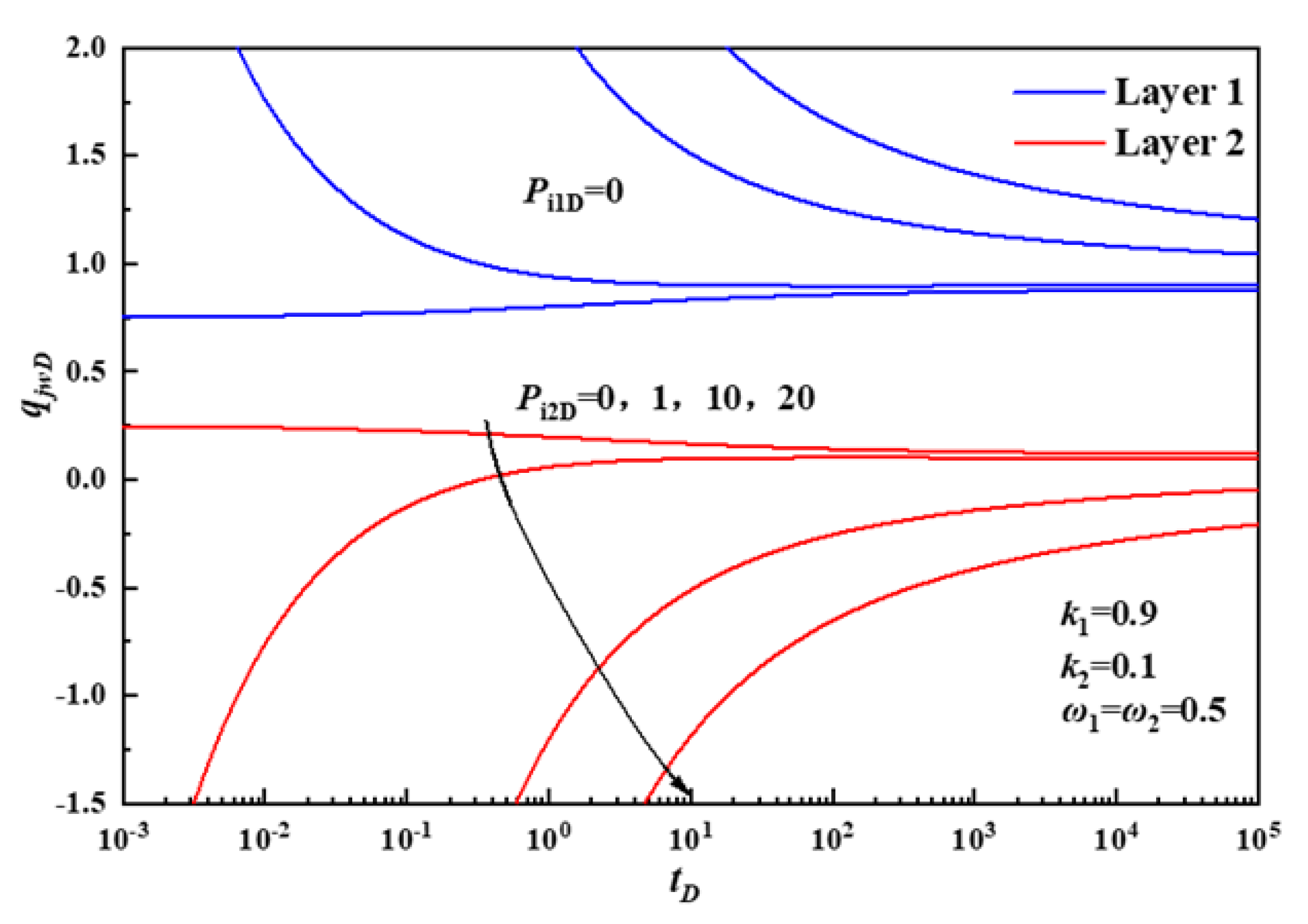
3.1.3. Dimensionless Initial Pressure

The results depicted in Figure 4 indicate that the initial pressure exhibits heterogeneity, leading to the occurrence of backflow during the early stages of well opening. The magnitude of backflow is directly proportional to both the permeability and pressure difference, while inversely proportional to the storage coefficient. Moreover, a greater disparity in initial pressure intensifies the severity of the backflow phenomenon. However, as mining time progresses, the bottom hole pressure decreases gradually, resulting in a rapid disappearance of backflow.

3.2. Case Example Analysis of Changqing Oil Field

3.2.1. Effect of Formation Parameters on Layered Contribution Rate
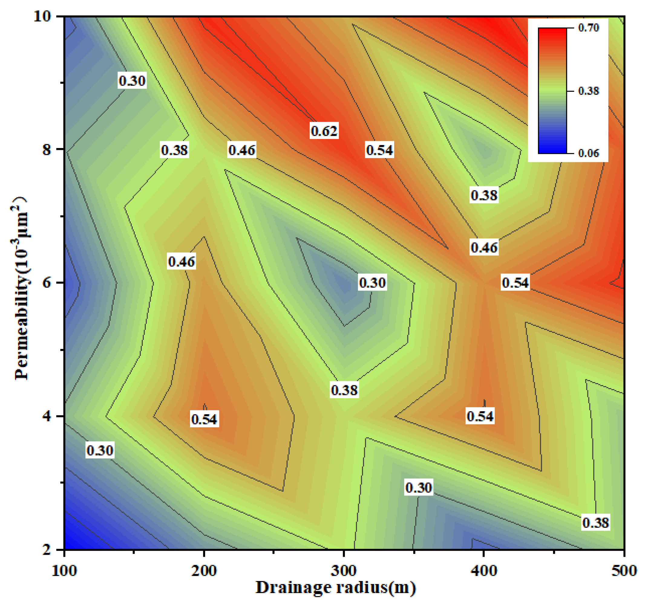
Taking the double-layer gas production well of a tight gas reservoir in the Changqing Oilfield as an example, the average daily gas production rate is 1 × 10⁴ m3/d. The thickness of the gas reservoir ranges from 2 to 10 m, with permeability varying between 2 and 10 × 10−3 μm2 and porosity ranging from 8% to 12%. The initial pressure of the low-pressure gas reservoir is 17.8 MPa, while that of the high-pressure gas reservoir is 18 MPa. Additionally, the drainage radius is 100–500 m. Based on these parameters’ distribution within four groups in the gas reservoir, five levels are designed for each group in the low-pressure gas reservoir, as shown in Table 1.
1
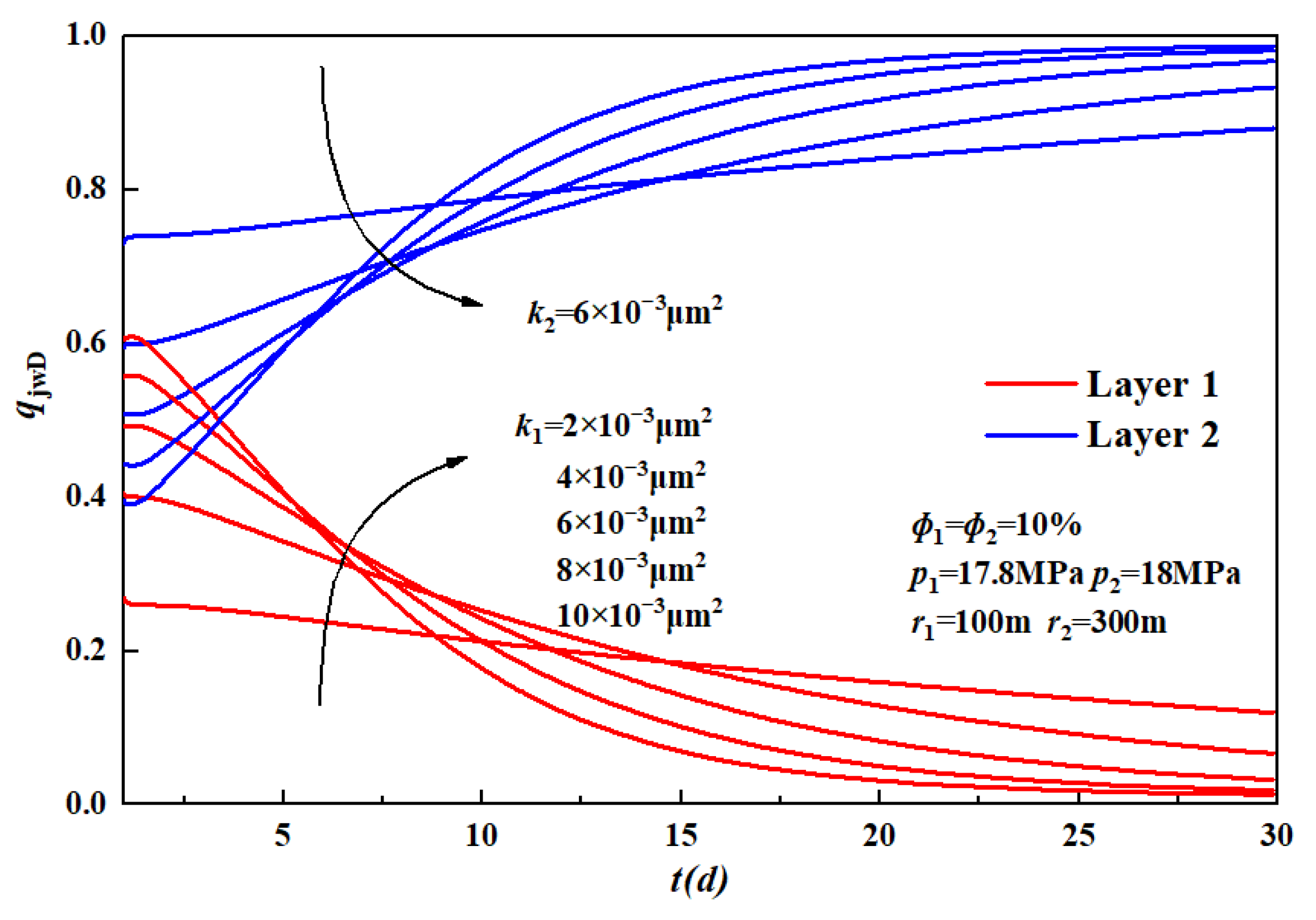
Effect of permeability on layered contribution rate.
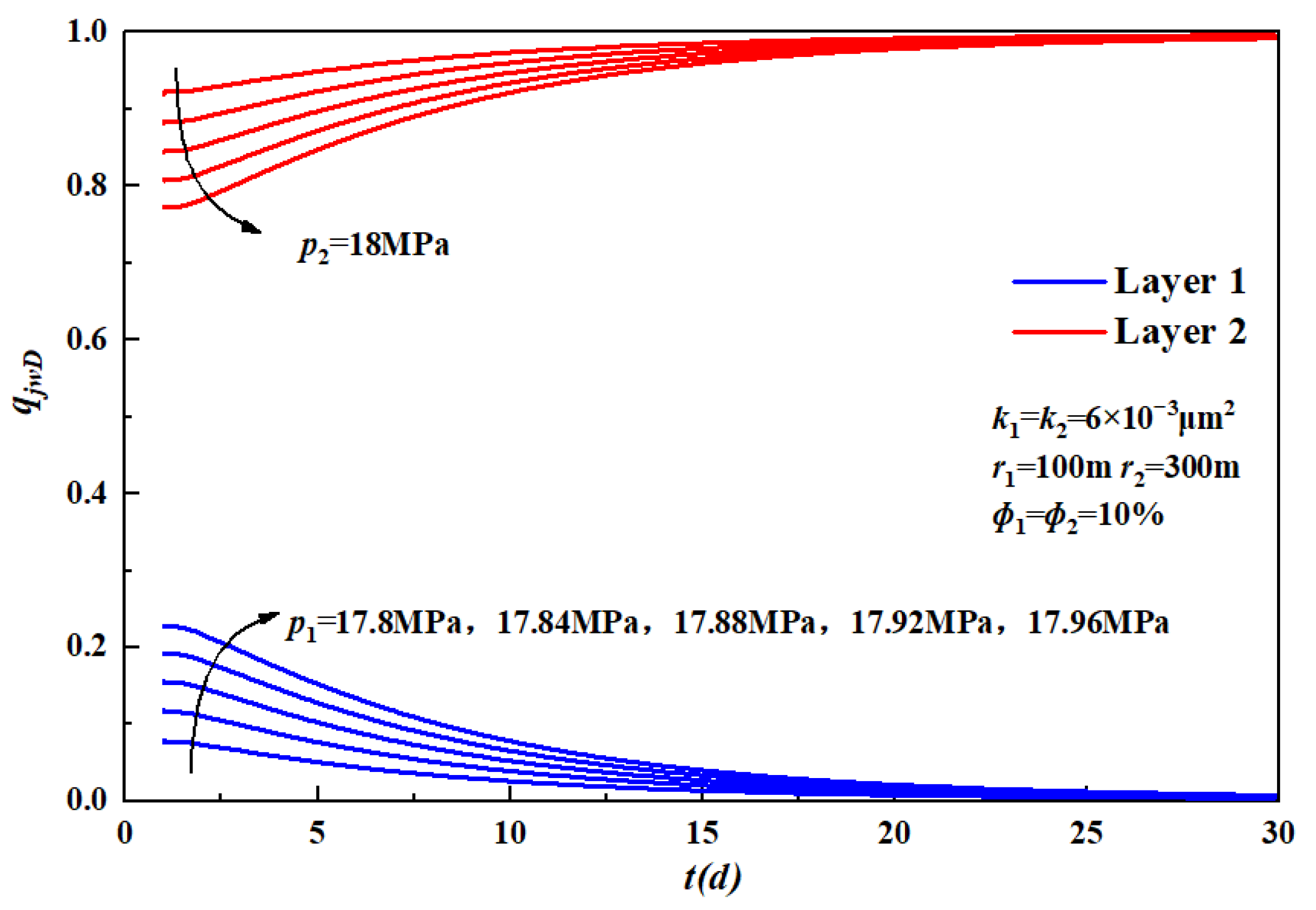
In order to investigate the influence of single-factor permeability on production in stratified gas wells, we designed parameters for a low-pressure gas reservoir and established five levels of permeability, as shown in Table 2.
Figure 5 shows the relationship between the layer flow and permeability at each layer with other parameters held constant. When the permeability of the low-pressure gas layer is lower than that of the high-pressure gas layer, the contribution of layer flow from the high-pressure gas layer surpasses that from the low-pressure gas layer throughout the entire production process. In cases where there exists a high-permeability low-pressure gas layer and a low-permeability high-pressure gas layer, the contribution curve of layer flow from the high-pressure gas layer intersects with that of the early stage in the production process, but the contribution of the layer flow of the high-pressure gas layer is generally higher in the whole production process.
2
Effect of initial pressure on layered contribution rate.
In order to study the influence of initial pressure on production in stratified gas wells, a low-pressure gas reservoir was selected as the experimental setting, with five different levels of initial pressure established as outlined in Table 3.
The relationship between the layer flow rate and the initial pressure at each layer, while keeping other parameters constant, is illustrated in Figure 6. With the increase in the initial pressure of the low-pressure gas layer, the pressure difference between the two layers decreases, the contribution of the low-pressure gas layer during early production stages gradually intensifies but diminishes in later stages. In the whole production process, there is generally a significant contribution from the high-pressure gas layer flow. Overall, it can be inferred that variations in the initial pressure of the low-pressure gas layer have a limited impact on its contribution to overall flow.
3
Effect of porosity on layered contribution rate.
In order to study the influence of single factor porosity on stratified gas well production, the parameters of the low-pressure gas reservoir were designed and five porosity levels were set, as shown in Table 4.
Figure 7 shows the relationship between the layer flow and porosity for each layer with other parameters held constant. With the increase in the porosity of the low-pressure gas reservoir, the contribution degree of the layer flow increases significantly in the middle production period, and there is little difference between the early and late production period. In general, the contribution degree of bed flow increases with the increase in porosity.
4
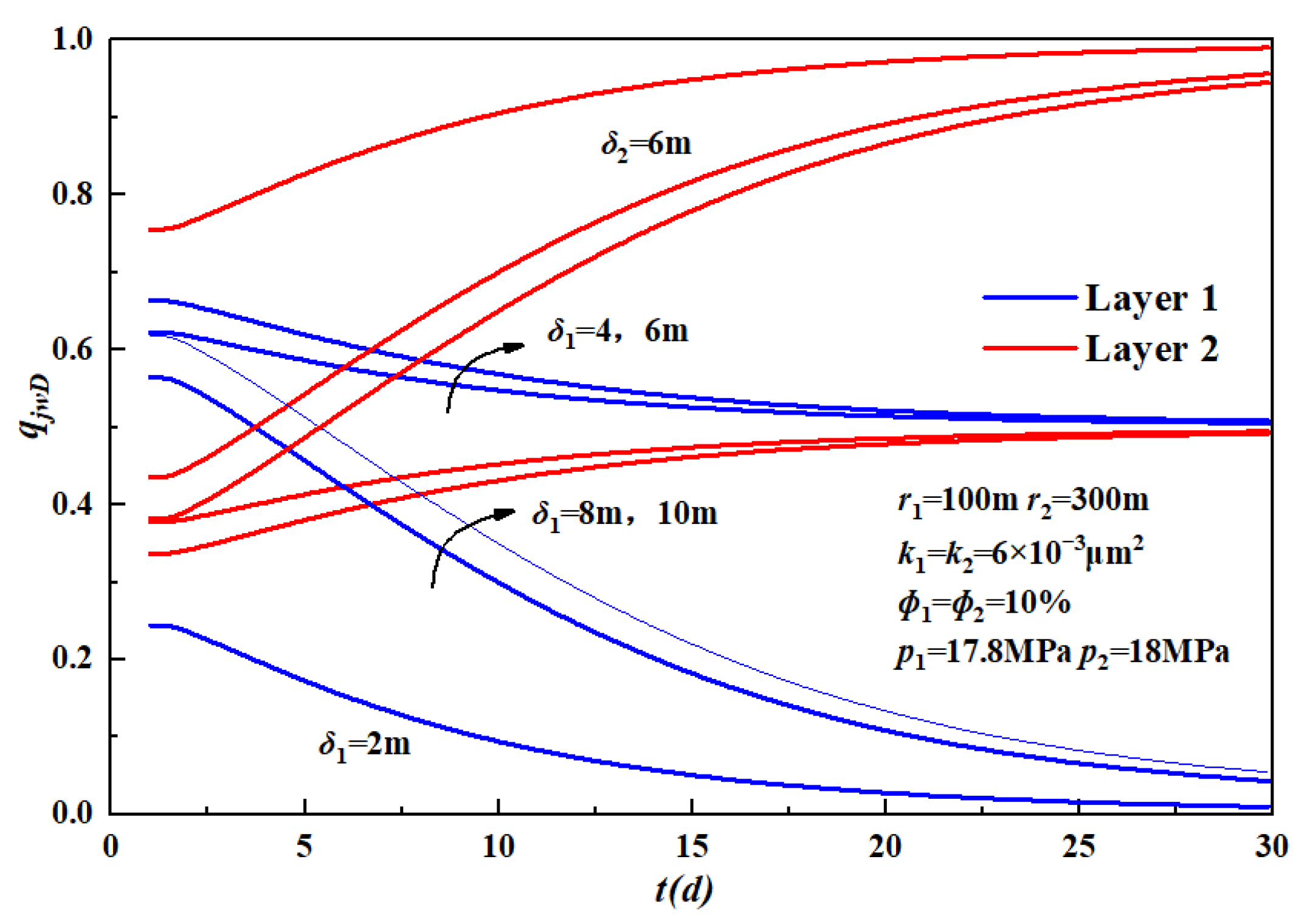
Effect of formation thickness on layered contribution rate.
In order to study the influence of single-factor layer thickness on stratified gas well production, the parameters of the low-pressure gas layer were designed, and five horizontal layers were set, as shown in Table 5.
Figure 8 shows the relationship between the layer flow and thickness of each layer with other parameters held constant. When the thickness difference between the two layers is ≥4 m, the high-pressure layer thickness exhibits a higher contribution to layer flow throughout the production process. Additionally, in the early stages of production, there is an intersection between the contribution curves of low-pressure layer thickness and low-pressure gas layer thickness. For a thickness difference of 2–4 m (i.e., when the low-pressure gas layer has a thickness of 4–6 m), the contribution degree of the low-pressure gas layer surpasses that of the high-pressure gas layer. Towards late production periods, both layers tend to have equal contributions with a degree close to 0.5.
5
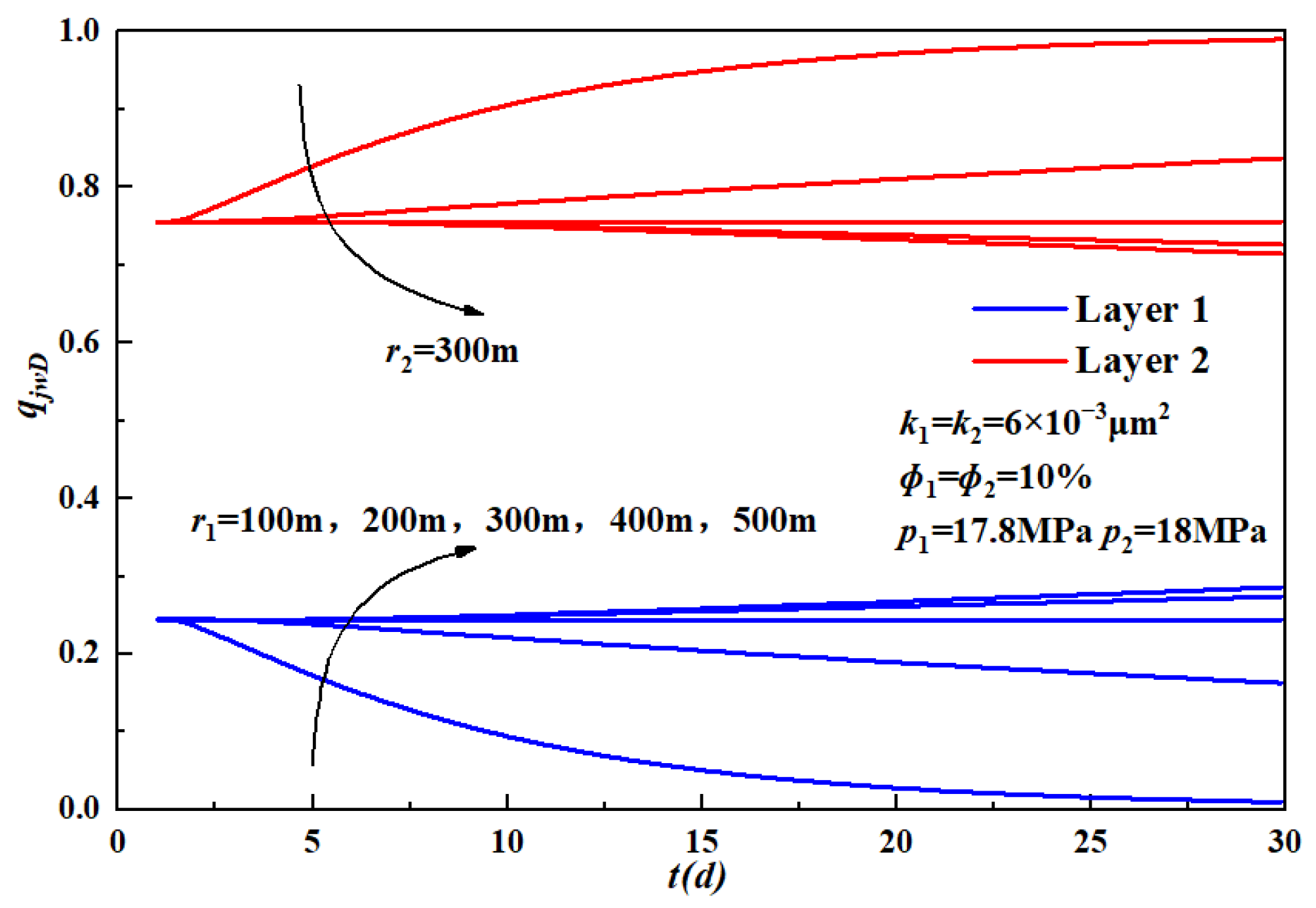
Effect of drainage radius on layered contribution rate.
In order to study the influence of single-factor drainage radius on stratified gas well production, the parameters of the low-pressure gas reservoir were designed, and five levels of drainage radius were set, as shown in Table 6.
Figure 9 shows the relationship between the layer flow and drainage radius for each layer with other parameters held constant. As the drainage radius of the low-pressure gas layer increases, the contribution degree of layer flow gradually rises; however, throughout the entire production process, the contribution degree of the high-pressure gas layer flow remains consistently higher than that of the low-pressure gas layer.

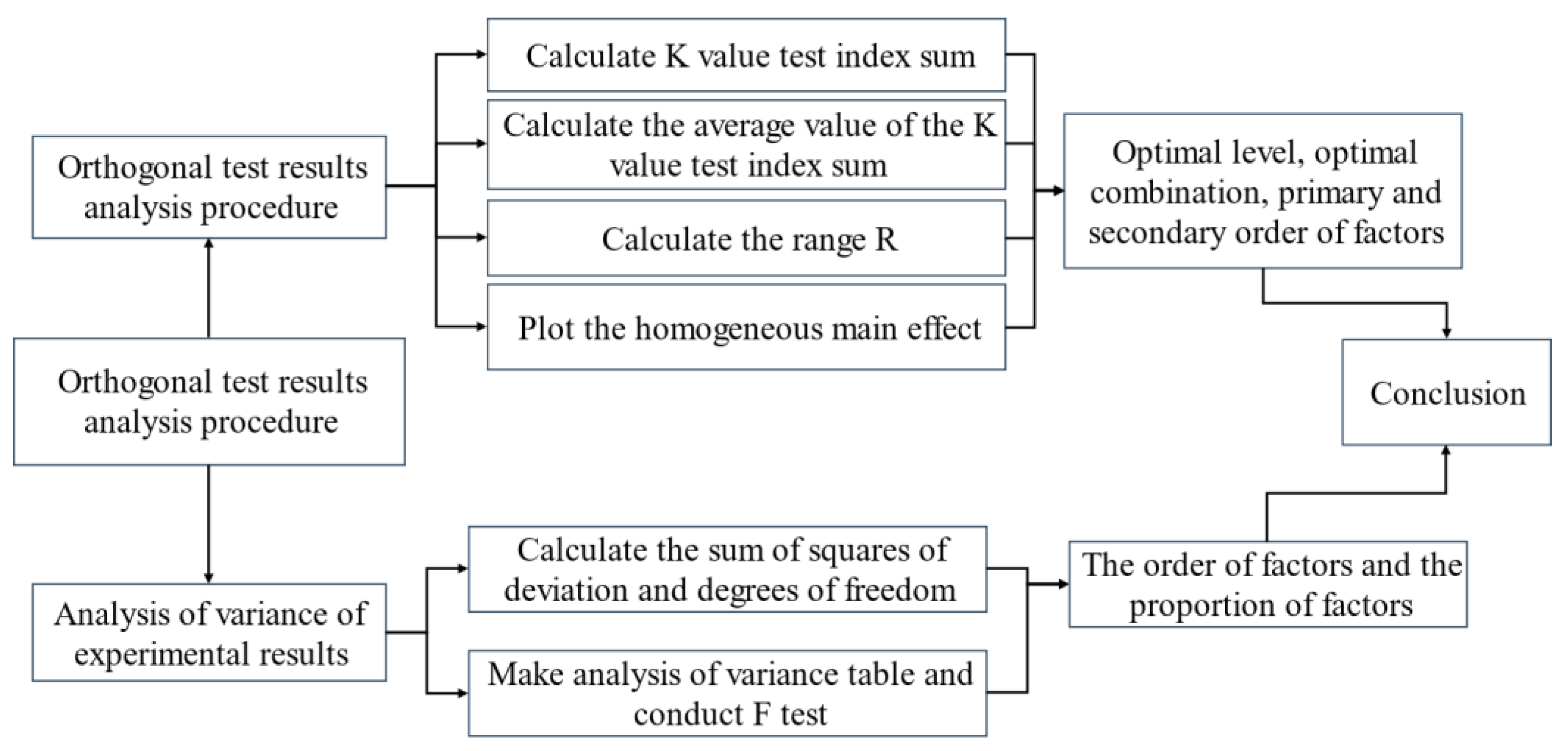
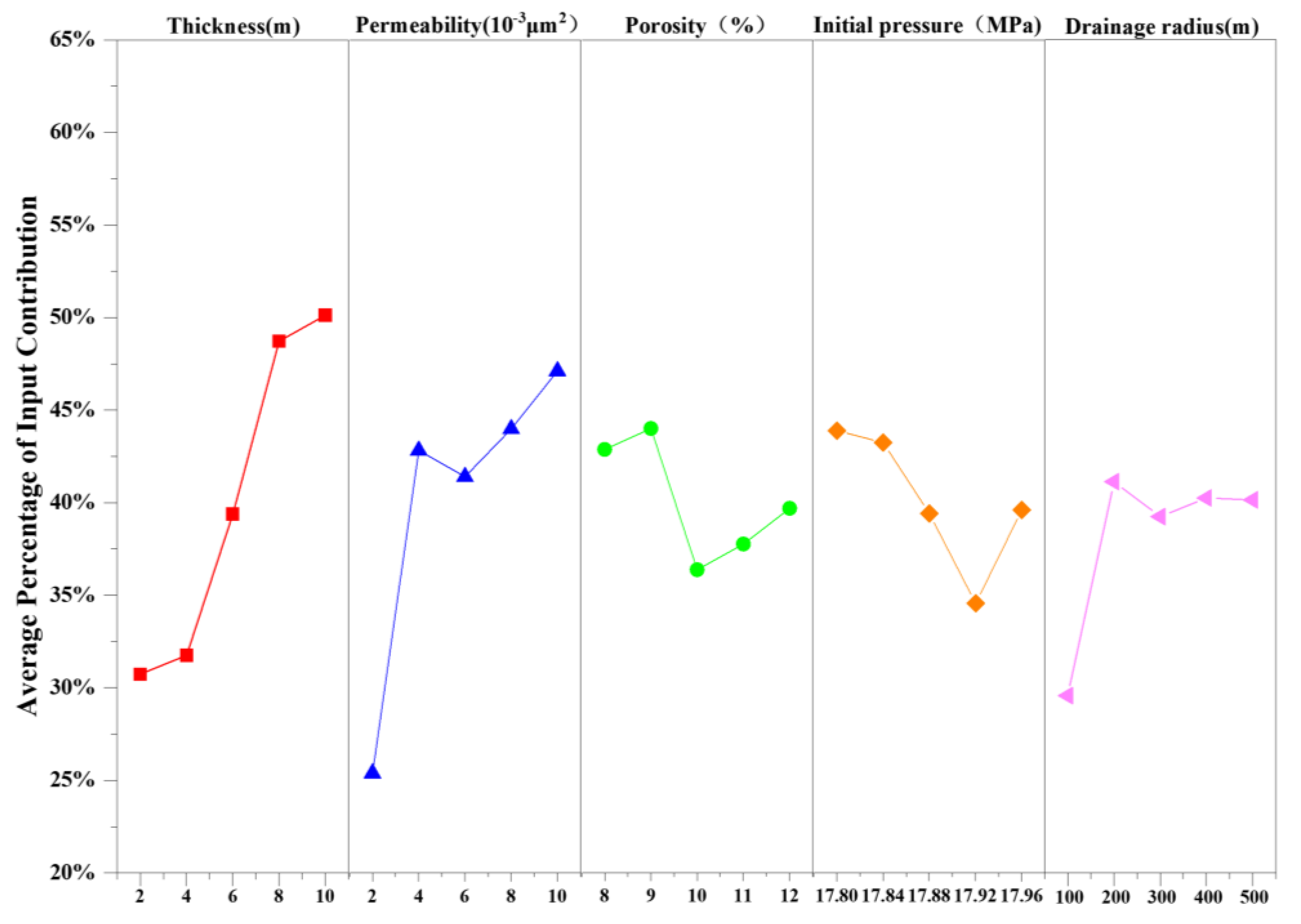
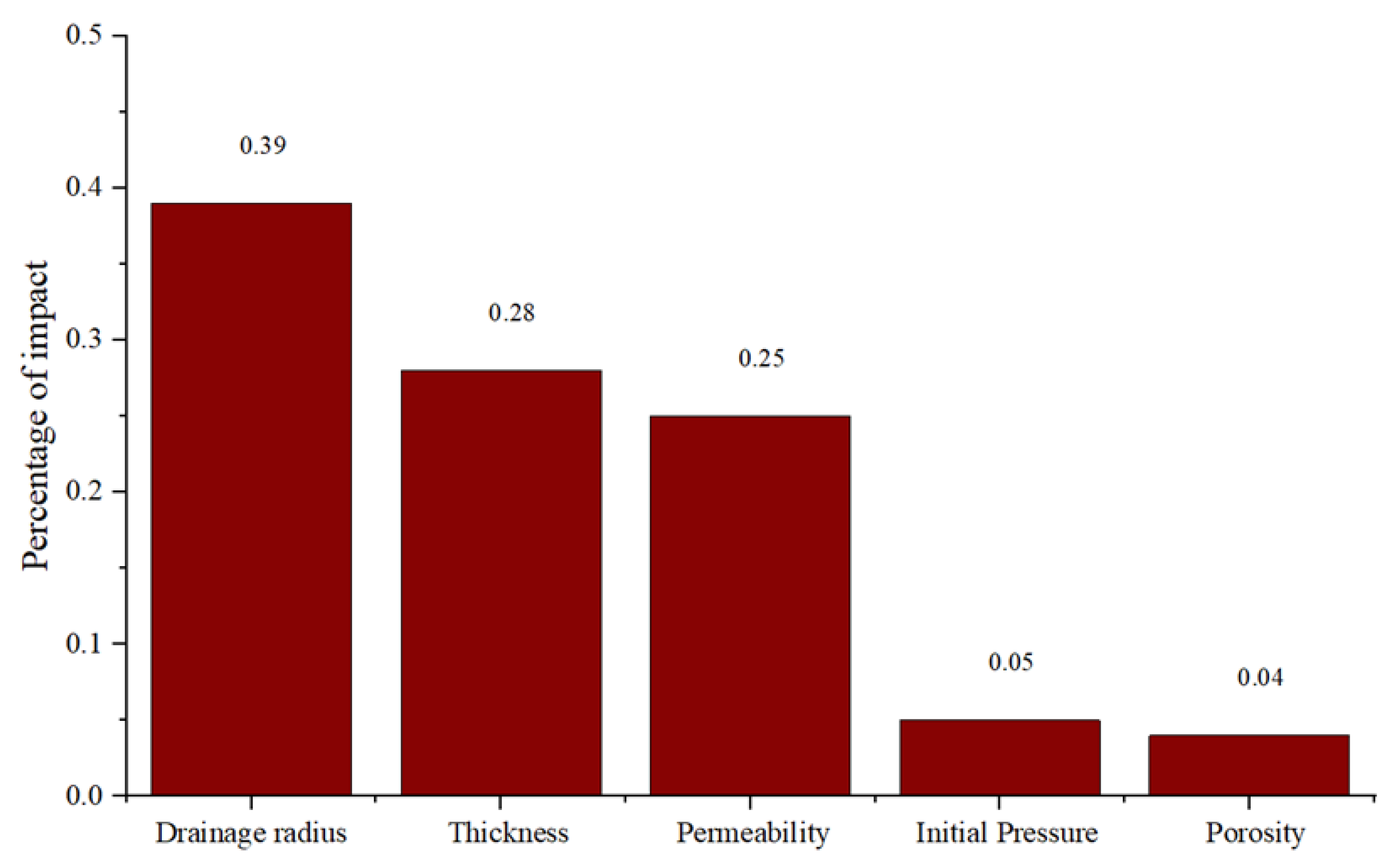
3.2.2. Multi-Factor Sensitivity Analysis

1
Orthogonal experiment design.
The orthogonal experimental design is a crucial discipline within statistical mathematics. The fundamental tool of the orthogonal method is the orthogonal table, which possesses two distinctive characteristics: (1) it ensures an equal number of different levels for each participating factor in the experiment and the number of combinations; (2) each level of any given factor exhibits closely comparable test conditions, enabling an effective comparison among factors. Therefore, employing orthogonal tables for experimental design not only reduces the number of experiments but also enhances their representativeness, thereby meeting the requirements of comprehensive experimentation more effectively.
High-pressure gas reservoir parameters were kept constant, and the contribution ratio of low-pressure gas reservoir production was taken as the test result, as shown in Table 7, to explore the proportion of each influencing factor under the interaction of multiple factors.
Subsequently, range analysis and analysis of variance were conducted on these results to determine the primary and secondary order of influencing factors, as well as the influence weight of the single-layer production contribution ratio under multiple influencing factors. The analytical process is illustrated in Figure 10.
2
Range analysis of orthogonal test results.
Through range analysis, a more intuitive comparison can be made between the primary and secondary factors influencing this test. The underlying principle is that variations in the k value, representing the average of i-level data for factor A, are generally attributed to different levels of factor A. The range (RA) between k values for different levels of factor A can be considered an approximate measure of how changes in factor A levels impact experimental results, with RA positively correlating with the significance of factor A.
The range analysis results are presented in Table 8, with the k value representing the average sum of each test index. Among them, the optimal levels are observed for the fifth level of thickness, the fifth level of permeability, the second level of porosity, the first level of initial pressure, and the second level of drainage radius. The range R indicates that the main and second order of influencing factors is drainage radius > permeability > thickness > initial pressure > porosity. Furthermore, the trend chart of contributing factors of gas reservoir production in Figure 11 also reflects the above conclusion. The three most important factors are drainage radius, permeability, and thickness, and porosity and initial pressure have little influence on production.
The isoline map presented in Figure 12 illustrates the contribution ratio of the two primary factors, namely the drainage radius and permeability, to the gas reservoir production. In this representation, the blue region is the area with a low contribution ratio, and the red area is the area with a high contribution ratio. As depicted in the figure, an increase in both drainage radius and permeability leads to a corresponding elevation in the production contribution ratio for this particular layer.
3
Variance analysis of Orthogonal test results.
Variance analysis is used to infer the significance of the difference in the overall mean value of the corresponding factors at different levels by analyzing the difference between the data fluctuation caused by each factor and the data fluctuation caused by the error. Given the complexity of this experiment involving multiple factors, batch numerical analysis software was employed for efficient processing of variance and range analyses in this study.
Table 9 shows the results of analysis of variance, where the F value represents the level of significance and the p value indicates the magnitude of difference. The findings reveal that the maximum F value of the drainage radius is 3.89, and the significance degree accounts for 38.71%, as shown in Figure 13. It was followed by thickness and permeability, whose F-values were 2.84 and 2.48, respectively, and the significant degree accounted for 28.26% and 24.68%. However, porosity and initial pressure do not exert significant influence on yield contribution. The order of importance for significant effects is as follows: drainage radius > thickness > permeability > initial pressure > porosity, and the three most important factors were drainage radius, permeability, and thickness, which was consistent with the results of range analysis.

4. Conclusions

(1) The paper establishes an unsteady seepage flow model for the combined production of multilayer gas reservoirs in vertical wells. By utilizing the Duhamel convolution principle, the variable flow problem is transformed into a constant flow problem. Subsequently, the Laplace spatial solution is obtained through Laplace transform, and finally, the real time-domain solution is derived using the Stehfest inversion. This comprehensive model takes into account various parameters such as permeability, reservoir thickness, porosity, and initial pressure to fully assess productivity.
(2) By integrating the unstable percolation model of multi-layer gas reservoirs with an orthogonal test design, this study comprehensively considers the proportion of each influencing factor under the combined influence of multiple factors. In the case of the double-layer gas production well of a tight gas reservoir in the Changqing Oilfield in this paper, where there is a small initial pressure difference between the gas reservoirs and no backflow phenomenon was found, it is found that the impact on productivity contribution is minimal due to the small permeability scale and span. The test results were analyzed through a combination of an orthogonal experimental design, range analysis, and variance analysis. The results of the range analysis and variance analysis indicate that the drainage radius has the greatest impact, followed by permeability, thickness, initial pressure, and porosity. The findings demonstrate that, within this gas reservoir, the dominant factors influencing productivity are the drainage radius, permeability, and thickness, whereas initial pressure and porosity exhibit a negligible impact on productivity.
(3) The model proposed in this paper provides valuable practical guidance for current multi-layer combined gas production reservoirs. It effectively orders the main and secondary influencing factors under the common influence of multi-layer gas reservoirs with different characteristics, thus offering theoretical guidance for subsequent joint drilling and abandonment of the secondary productive contribution layer in multi-layer gas reservoirs.

Author Contributions

Conceptualization, L.W. and Y.X.; methodology, L.W. and Y.X.; validation, H.T., L.W. and Y.X.; formal analysis, H.T. and Y.X.; investigation, H.T.; data curation, H.T. and J.K.; writing—original draft preparation, H.T. and L.W.; writing—review and editing, L.W; visualization, H.T. and L.W.; supervision, L.W.; project administration, L.W. and J.K. All authors have read and agreed to the published version of the manuscript.

Funding

This work is supported by Open Fund Project “Study on Multiphase Flow Semi-Analytical Method for Horizontal Wells of Continental Shale Condensate Gas” of Sinopec Key Laboratory of Shale Oil/Gas Exploration and Production Technology (Grant No. 33550000-22-ZC0613-0208).

Data Availability Statement

The data presented in this study are available on request from the corresponding authors. The data are not publicly available due to the continuation of a follow-up study by the authors.

Conflicts of Interest

The authors declare no conflict of interest.

References

  1. Kong, X. Advanced Seepage Mechanics, 3rd ed.; University of Science and Technology of China Press: Hefei, China, 2020. [Google Scholar]
  2. Zhang, M.Y. Numerical Simulation of Factors Affecting Productivity of Multi-Layer Fractured Straight Wells in Tight Gas Reservoirs; Yangtze University: Wuhan, China, 2016. [Google Scholar]
  3. Lefkovits, H.C.; Hazebroek, P.; Allen, E.E.; Matthews, C.S. A study of the behavior of bounded reservoirs composed of stratified layers. Soc. Pet. Eng. J. 1961, 1, 43–58. [Google Scholar] [CrossRef]
  4. Russell, D.G.; Prats, M. Performance of Layered Reservoirs with Crossflow Single Compressible Fluid Case. Soc. Pet. Eng. J. 1962, 2, 53–67. [Google Scholar] [CrossRef]
  5. Russell, D.G.; Prats, M. The Practical Aspects of Interlayer Crossflow. J. Pet. Technol. 1962, 14, 589–594. [Google Scholar] [CrossRef]
  6. Papadopulos, I.S. Nonsteady flow to multiaquifer wells. J. Geophys. Res. 1966, 71, 4791–4797. [Google Scholar] [CrossRef]
  7. Kucuk, F.; Ayestaran, L. Analysis of simultaneously measured pressure and sandface flow rate in transient well testing (includes associated papers 13937 and 14693). J. Pet. Technol. 1985, 37, 323–334. [Google Scholar] [CrossRef]
  8. Kucuk, F.; Karakas, M.; Ayestaran, L. Well testing and analysis techniques for layered reservoirs. SPE Form. Eval. 1986, 1, 342–354. [Google Scholar] [CrossRef]
  9. Tariq, S.M.; Henry, J.R. Drawdown behavior of a well with storage and skin effect communicating with layers of different radii and other characteristics. In Proceedings of the SPE Annual Fall Technical Conference and Exhibition, Houston, TX, USA, 1–3 October 1978. [Google Scholar]
  10. Larsen, L. Wells producing commingled zones with unequal initial pressures and reservoir properties. In Proceedings of the SPE Annual Technical Conference and Exhibition, San Antonio, TX, USA, 4–7 October 1981. [Google Scholar]
  11. Bourdet, D. Pressure behavior of layered reservoirs with crossflow. In Proceedings of the SPE California Regional Meeting, Bakersfield, CA, USA, 27–29 March 1985. [Google Scholar]
  12. Mavor, M.J.; Walkup, G.W., Jr. Application of the parallel resistance concept to well test analysis of multilayered reservoirs. In Proceedings of the SPE California Regional Meeting, Oakland, CA, USA, 2–4 April 1986. [Google Scholar]
  13. Rahman, N.M.A.; Mattar, L. New analytical solution to pressure transient problems in commingled, layered zones with unequal initial pressures subject to step changes in production rates. J. Pet. Sci. Eng. 2007, 56, 283–295. [Google Scholar] [CrossRef]
  14. Spath, J.B.; Ozkan, E.; Raghavan, R. An efficient algorithm for computation of well responses in commingled reservoirs. SPE Form. Eval. 1994, 9, 115–121. [Google Scholar] [CrossRef]
  15. Milad, B.; Civan, F.; Devegowda, D.; Sigal, R.F. Modeling and simulation of production from commingled shale gas reservoirs. In Proceedings of the SPE/AAPG/SEG Unconventional Resources Technology Conference, Denver, CO, USA, 12–14 August 2013. [Google Scholar]
  16. Agarwal, B.; Chen, H.Y.; Raghavan, R. Buildup behaviors in commingled reservoir systems with unequal initial pressure distributions: Interpretation. In Proceedings of the SPE Annual Technical Conference and Exhibition, Washington, DC, USA, 4–7 October 1992. [Google Scholar]
  17. Hatzignatiou, D.G.; Ogbe, D.O. Interference pressure behavior in stratified reservoirs. In Proceedings of the SPE Western Regional Meeting, Anchorage, AK, USA, 26–28 May 1993. [Google Scholar]
  18. Sahni, A.; Hatzignatiou, D.G.; Ogbe, D.O. Interference pressure behavior in multilayered faulted reservoirs. In Proceedings of the SPE Western Regional Meeting, Anchorage, AK, USA, 22–24 May 1996. [Google Scholar]
  19. Ei-Banb, A.H.; Wattenbarger, R.A. Analysis of commingled tight gas reservoirs. In Proceedings of the SPE Annual Technical Conference and Exhibition, Denver, CO, USA, 6–9 October 1996. [Google Scholar]
  20. Arevalo-Villagran, J.A.; Wattenbarger, R.A.; El-Banbi, A.H. Production analysis of commingled gas reservoirs-case histories. In Proceedings of the SPE International Petroleum Conference and Exhibition in Mexico, Villahermosa, Mexico, 1–3 February 2000. [Google Scholar]
  21. Zhang, S.Q.; Zhang, W.J.; Zhang, S.G. Influence of interzonal interference on gas test. Oil Gas Well Test. 1996, 3, 42–45. [Google Scholar]
  22. Wang, Y.; He, Z.X.; Wang, R.C.; Li, X.C. Determination of interlayer interference coefficient of multi-layer combined production in low permeability gas reservoir. Sci. Technol. Eng. 2012, 20, 9163–9166. [Google Scholar]
  23. Zhang, S.; Liu, Z.; Shi, A.; Wang, X. Development of accurate well models for numerical reservoir simulation. Adv. Geo-Energy Res. 2019, 3, 250–257. [Google Scholar] [CrossRef]
  24. Xian, B.; Xiong, Y.; Shi, G.X.; Li, P.C.; Chen, M. Study on interlayer interference analysis and technical countermeasures of combined production in thin reservoir. Spec. Oil Gas Reserv. 2007, 14, 51–54. [Google Scholar]
  25. Liu, Q.G.; Wang, H.; Shi, G.X.; Wang, R.C.; Li, X.C. Calculation method and influencing factors of stratified production contribution of multi-layer gas reservoir. J. Southwest Pet. Univ. Nat. Sci. Ed. 2010, 32, 80. [Google Scholar]
  26. Luo, H.; Mahiya, G.F.F.; Pannett, S. The use of rate-transient-analysis modeling to quantify uncertainties in commingled tight gas production-forecasting and decline-analysis parameters in the alberta deep basin. SPE Reserv. Eval. Eng. 2014, 17, 209–219. [Google Scholar] [CrossRef]
  27. Yang, X.F.; Liu, Y.C.; Jin, L.; Ying, W.; Hui, D. Effect of separate layer recovery or multilayer commingled production and the optimal selection of development methods for two-layer gas reservoirs. Nat. Gas Ind. 2012, 32, 57–60. [Google Scholar]
  28. Santiago, V.; Ribeiro, A.; Hurter, S. Modeling the contribution of individual coal seams on commingled gas production. SPE Prod. Oper. 2021, 36, 245–261. [Google Scholar] [CrossRef]
  29. Huang, S.; Kang, B.; Cheng, L.; Zhou, W.; Chang, S. Quantitative characterization of interlayer interference and productivity prediction of directional wells in the multilayer commingled production of ordinary offshore heavy oil reservoirs. Pet. Explor. Dev. 2015, 42, 533–540. [Google Scholar] [CrossRef]
  30. Zhao, Y.; Zhao, L.; Cheng, L.; Wang, Z.; Yang, H. Numerical simulation of multi-seam coalbed methane production using a gray. J. Pet. Sci. Eng. 2018, 175, 587–594. [Google Scholar] [CrossRef]
  31. Yan, B.; Wang, Y.; Killough, J.E. Beyond dual-porosity modeling for the simulation of complex flow mechanisms in shale reservoirs. Comput. Geoences 2016, 20, 69–91. [Google Scholar] [CrossRef]
  32. Wang, Y.; Yan, B.; John, K. Compositional Modeling of Tight Oil Using Dynamic Nanopore Properties. In Proceedings of the SPE Annual Technical Conference and Exhibition, New Orleans, LA, USA, 30 September–2 October 2013. [Google Scholar]
  33. Yan, B.; Li, C.; Killough, J.E. A Fully Compositional Model Considering the Effect of Nanopores in Tight Oil Reservoirs. J. Pet. Ence Eng. 2017, 152, 675–682. [Google Scholar] [CrossRef]
  34. Yan, B.; Wang, Y.; Tariq, Z.; Zhang, K. Estimation of heterogeneous permeability using pressure derivative data through an inversion neural network inspired by the Fast Marching Method. Geoenergy Sci. Eng. 2023, 228, 211982. [Google Scholar] [CrossRef]
  35. Tariq, Z.; Gudala, M.; Yan, B.; Sun, S.; Rui, Z. Optimization of Carbon-Geo Storage into Saline Aquifers: A Coupled Hydro-Mechanics-Chemo Process. In Proceedings of the SPE EuropEC—Europe Energy Conference featured at the 84th EAGE Annual Conference & Exhibition, Vienna, Austria, 5–8 June 2023. [Google Scholar]
  36. Xu, Z.; Yan, B.; Gudala, M.; Rui, Z.; Tariq, Z. A Robust General Physics-Informed Machine Learning Framework for Energy Recovery Optimization in Geothermal Reservoirs. In Proceedings of the SPE EuropEC—Europe Energy Conference featured at the 84th EAGE Annual Conference & Exhibition, Vienna, Austria, 5–8 June 2023. [Google Scholar]
  37. Tariq, Z.; Ertugrul, U.Y.; Gudala, M.; Yan, B.; Sun, S.; Hussein, H. Spatial–temporal prediction of minerals dissolution and precipitation using deep learning techniques: An implication to Geological Carbon Sequestration. Fuel 2023, 341, 127677. [Google Scholar] [CrossRef]
  38. Yan, B.; Xu, Z.; Gudala, M.; Tariq, Z.; Finkbeiner, T. Reservoir Modeling and Optimization Based on Deep Learning with Application to Enhanced Geothermal Systems. In Proceedings of the SPE Reservoir Characterisation and Simulation Conference and Exhibition, Abu Dhabi, UAE, 24–26 January 2023. [Google Scholar]
Figure 1. Schematic diagram for physical model of multi-layer combined production.
Water 15 03052 g001
Figure 2. The effect of storage coefficient (ω) on the contribution of stratification under different permeability coefficients: (a) the permeability coefficients of the first and second layers (k1 and k2) are 0.5 and 0.5, respectively, (b) the permeability coefficients of the first and second layers (k1 and k2) are 0.1 and 0.9, respectively, and (c) the permeability coefficients of the first and second layers (k1 and k2) are 0.9 and 0.1, respectively.
Water 15 03052 g002aWater 15 03052 g002b
Figure 3. The effect of permeability coefficient (k) on the contribution of stratification under different storage coefficients: (a) the storage coefficients of the first and second layers (ω1 and ω2) are 0.5 and 0.5, respectively, (b) the storage coefficients of the first and second layers (ω1 and ω2) are 0.1 and 0.9, respectively, and (c) the storage coefficients of the first and second layers (ω1 and ω2) are 0.9 and 0.1, respectively.
Water 15 03052 g003
Figure 4. The effect of dimensionless initial pressure (PiD) on the contribution of stratification.
Water 15 03052 g004
Figure 5. The effect of permeability on the contribution of stratification.
Water 15 03052 g005
Figure 6. Surface flow chart of dual-layer gas reservoir with different initial pressures (Pi).
Water 15 03052 g006
Figure 7. Surface flow chart of double-layer gas reservoir with different porosity (ɸ).
Water 15 03052 g007
Figure 8. Layer flow chart of two-layer gas reservoir with different layer thickness (δ).
Water 15 03052 g008
Figure 9. Surface flow chart of different drainage radius of two-layer gas reservoir (r).
Water 15 03052 g009
Figure 10. Flow chart of orthogonal test result analysis.
Water 15 03052 g010
Figure 11. Trend chart of factors contributing to gas reservoir production.
Water 15 03052 g011
Figure 12. Contour map of production contribution proportion of gas reservoir (drainage radius and permeability).
Water 15 03052 g012
Figure 13. Analysis of variance impact percentage histogram.
Water 15 03052 g013
Table 1. Parameter design table of low-pressure gas reservoir.
LevelThickness
(m)
Permeability
(10−3 μm2)
Porosity
(%)
Initial Pressure
(MPa)
Drainage Radius (m)
122817.80100
244917.84200
3661017.88300
4881117.92400
510101217.96500
Table 2. Design table of permeability parameters of low-pressure gas reservoir.
Thickness
(m)
Porosity
(%)
Initial Pressure
(MPa)
Drainage Radius
(m)
Permeability (10−3 μm2)
2817.80100246810
Table 3. Design table of initial pressure parameters of low-pressure gas reservoir.
Thickness
(m)
Porosity
(%)
Permeability
(10−3 μm2)
Drainage Radius
(m)
Initial Pressure (MPa)
28610017.817.8417.8817.9217.96
Table 4. Design table of low-pressure gas reservoir porosity parameters.
Thickness
(m)
Initial Pressure
(MPa)
Permeability
(10−3 μm2)
Drainage Radius
(m)
Porosity (%)
217.8610089101112
Table 5. Low-pressure gas thickness parameter design table.
Porosity
(%)
Initial Pressure
(MPa)
Permeability
(10−3 μm2)
Drainage Radius
(m)
Thickness (m)
817.86100246810
Table 6. Design table of low-pressure gas reservoir drainage radius parameters.
Porosity
(%)
Initial Pressure
(MPa)
Permeability
(10−3 μm2)
Thickness (m)Drainage Radius (m)
817.86100100200300400500
Table 7. Orthogonal experiment design table for multi-factor analysis.
The CaseThickness
(m)
Permeability
(10−3 μm2)
Porosity
(%)
Initial Pressure
(MPa)
Drainage Radius
(m)
Production Contribution
122817.81006.74%
224917.8420054.53%
3261017.8830024.67%
4281117.9240031.18%
52101217.9650036.56%
642917.8840020.21%
7441017.9250032.87%
8461117.9610018.59%
9481217.820040.24%
10410817.8430046.90%
11621017.9620026.84%
12641117.830041.26%
13661217.8440051.32%
14680817.8850057.22%
156100917.9210020.31%
16821117.8450033.86%
17841217.8810031.09%
1886817.9220049.14%
1988917.9630061.67%
208101017.840067.88%
211021217.9230039.30%
22104817.9640054.40%
23106917.850063.31%
241081017.8410029.62%
2510101117.8820063.96%
Table 8. Range analysis results.
LevelThicknessPermeabilityPorosityInitial PressureDrainage Radius
k value10.30740.25390.42880.43890.2127
20.31760.42830.44010.43250.4694
30.39390.41410.36380.39430.4276
40.48730.43990.37770.34560.4500
50.50120.47120.39700.39610.4476
Range R0.19380.21730.07630.09330.2567
Ranking of impact degree32541
Table 9. Analysis of variance results.
Sources of VarianceDegrees of FreedomDeviation Sum of SquaresVarianceF Valuep ValueDegree of Significance
Thickness40.166230.0415572.840.168*
permeability40.144950.0362372.480.200*
Porosity40.021210.0053040.360.825Δ
Initial pressure40.027810.0069530.480.755Δ
Drainage radius40.227110.0567783.890.108*
Error40.058430.014607
Note: ‘*’ means moderately significant, and ‘Δ’ means not significant.
Disclaimer/Publisher’s Note: The statements, opinions and data contained in all publications are solely those of the individual author(s) and contributor(s) and not of MDPI and/or the editor(s). MDPI and/or the editor(s) disclaim responsibility for any injury to people or property resulting from any ideas, methods, instructions or products referred to in the content.

