1. Introduction
The natural boundary is intuitively understood to be the line dividing the bed of a lake, river, or sea from the adjacent land. Though different terminology (e.g., natural boundary, ordinary high water mark, riparian boundary, etc.) and definition specifics may be used, the concept is employed in many jurisdictions to define the boundary of ownership between a land parcel and a state-owned watercourse. The concept originates in British Common Law and accepts the ambulatory nature of waterways. It is typically defined on the ground by a professional surveyor based on evidence of the presence and action of water and its impact on the vegetation and soil of the shoreline.
The natural boundary is expected to change over time, and the loss or gain to adjacent property owners is accepted if slow and imperceptible, and if caused by natural forces of erosion or accretion. However, many jurisdictions include legal provisions that disregard human impacts to the natural boundary. While this makes sense in the context of earthworks which impact the shoreline, it is still unclear how the courts will interpret these provisions in the context of anthropogenic climate change.
There are many scenarios where estimating changes to the natural boundary may be important for investment, management, or regulatory decision making: consider, for example, a lake under prolonged drought conditions, the seashore with sea level rise, or riverfront with changes to upstream flow regulation. However, the observational nature of natural boundary surveying does not lend itself to exploring the impact of these “what if?” scenarios. It is apparent that practical tools would be useful to project changes to the natural boundary under different water regulation and change climate conditions.
Estimating changes to shoreline morphology due to changing water levels and/or wind and wave conditions (i.e., the hydrologic climate) is not a new problem. Two basic approaches are generally used. The first is based on observational data. Many studies have focused on estimating horizontal shoreline recession rates based on past observations and projecting the observed rates into the future (e.g., [
1]). However, by using past observations to predict future shoreline change, this approach inherently assumes climate stationarity. This does not address the problem of projecting shoreline change under different possible climate scenarios.
The other approach to estimating shoreline change is process-based. That is, estimating shoreline change based on the dominant climatic conditions driving that change. Numerous studies have linked wave climate to erosion rates. Studies focusing on highly mobile sediments, such as sand dunes, tend to identify large wave events, or groups of events as the primary driver of erosion (e.g., [
2]). Studies focusing on less mobile substrates such as saltmarsh or bedrock tend to identify the average wave conditions as the primary driver of erosion (e.g., [
3]). Some studies also recognize the importance of prevailing water levels in combination with waves in driving erosion [
4]. Some works have proposed wave energy limits for maintaining stable salt marsh [
5,
6]; however, these limits are site and vegetation species-specific. Leonardi et al. [
7] propose a simple linear relationship between average wave power and erosion in coastal wetlands. While these studies help to understand the relationship between the hydrologic climate and erosion, they do not provide a general basis for estimating natural boundary change.
The classical approach to estimating shoreline change in response to a change in water levels is the Bruun Rule [
8]. This approach involves significant simplifications of the wave climate and the beach profile and is generally only applicable to sandy beaches. Further, this approach requires that the wave climate remains constant, and the water level regime is transformed with a simple offset, which is generally not the case in estuarine, riverine, and lake environments.
Studies of shoreline erosion in response to water level change are commonly performed when evaluating potential impacts of creating hydroelectrical reservoirs. These techniques (e.g., [
9,
10]) are empirical in nature and predict the volume of material that would erode for a given effective wave energy and shore zone geometry and, thereby, predict the bluff or shoreline recession distance. These techniques have been developed for large changes in water level where the modified water level regime is significantly different than the range of existing water levels, and are primarily based on the down-cutting erosion mechanism.
Given the legal importance of the natural boundary in many jurisdictions, there is a surprising lack of published research aimed at understanding what determines its location. It is obviously related to the erosive power of water and waves, as well as the impact of prolonged submersion on plant species. However, there are few published studies relating these drivers to the natural boundary location. Some professionals in the fields of surveying and planning have raised concerns with the implications of our current use of the natural boundary in a changing climate [
11,
12,
13], highlighting the need for tools for estimating potential natural boundary change.
The present work uses a case study of a large lake (Cowichan Lake) to explore the relationship between the shoreline morphology and the hydrologic climate and the elevation of the natural boundary. The use of the natural boundary elevation as a metric for assessing shoreline morphologic change is assessed. Two process-based methods for estimation of the natural boundary change are proposed, one based on the observed statistical relationship between the shoreline morphology, the hydrologic climate, and the natural boundary elevation, and another method based on detailed analytical modelling of bottom stress from breaking waves. While observational data are not available to support evaluation of these methods, the results are evaluated by comparison of the results.
Section 2 of this paper describes the study site of Cowichan Lake.
Section 3 provides additional background on how the natural boundary is identified in the field.
Section 4 presents the methods, data, and models that were used to assess the physical characteristic of the lake and shoreline.
Section 5 provides an analysis of the hydrologic climate of the lake, presents a regression analysis of the data, refines the hypothesis, and proposes two approaches for estimating natural boundary change.
Section 6 presents and discusses the application of the proposed approaches to the Cowichan Lake shoreline.
Section 7 summarizes the most important findings of this work and provides some concluding remarks.
2. Study Site
Cowichan Lake is located on Vancouver Island, British Columbia, Canada and has a length of about 32 km, a maximum width of 4 km, a maximum depth of about 160 m, and a perimeter of approximately 100 km. The Villages of Lake Cowichan, Youbou, and Honeymoon Bay are situated on the lake’s shore. The lake is a popular site for summertime recreation, and most of the 700+ developed shoreline properties include beach or dock access. However, much of the lakeshore, especially to the northwest, is bordered by forest resource lands and is currently undeveloped. Cowichan Lake is at the head of the Cowichan Valley and is the source of the Cowichan River. The lake is surrounded by mountainous forested terrain, except to the southeast, along which runs the axis of the Cowichan Valley. The surficial geology of the area is primarily consolidated by the Vashon Drift including till, glacial sand, gravel and cobble, deposited during the last glacial period. There are also several large bedrock outcrops.
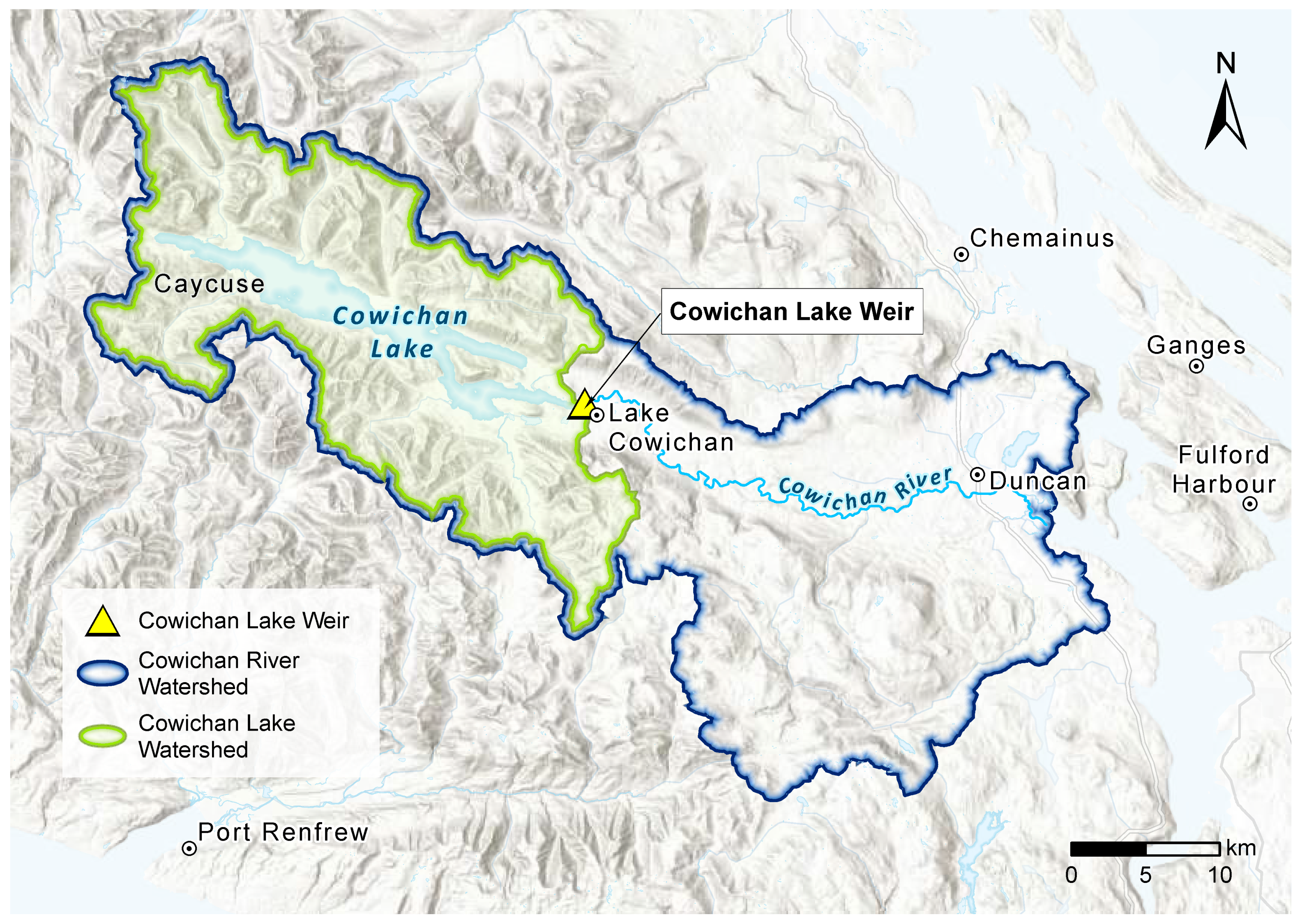
Cowichan Lake water levels are regulated at the outlet to the Cowichan River by a weir and gate system (see
Figure 1). This system is used to store water from the rainy spring season and to capture spring snow-melt as a source to supplement river flows during the dry summer season. This ensures a supply of base levels of river flow to support environmental health and allow the drawing of water from the river for residential and industrial uses. Since the 1960s, spring and summer inflows into the lake have decreased, and further decreases are expected with climate change [
14]. The storage provided by the system is now often insufficient to maintain base flows through the summer and early fall, and an upgrade of the weir system to increase storage is being proposed. The proposed upgrades would raise the weir by 70 cm and initiate regulation earlier in the spring season. However, the control gates would remain open during the fall and winter storm season, so that lake levels are not expected to increase substantially during this period.
3. Background on the Natural Boundary
The definition of the natural boundary used in this work is that found in the Land Act of the Province of British Columbia:
“Natural boundary” means the visible high-water mark of any lake, river, stream, or other body of water where the presence and action of the water are so common and usual, and so long continued in all ordinary years, as to mark on the soil of the bed of the body of water a character distinct from that of its banks, in vegetation, as well as in the nature to the soil itself.
Shorelines can be classified based on their predominant sediment type as: silt, sand, gravel, cobble, boulder, and bedrock. The most commonly occurring are gravel and cobble shorelines. For these shorelines, fines, organics, and the associated nutrients are eroded from the beach surface by the action of waves; consequently, the beach face below the natural boundary is rendered sterile to most plant species. In these cases, the location of the natural boundary is a dominated by the action of water and may represent a relatively wide transition zone between the sterile beach face and established non-aquatic vegetation on the backshore.
Typically, the action of water also defines the natural boundary location for bedrock shores; however, unlike gravel, the vegetation tends to change quickly with elevation such that the natural boundary is demarked by a sharp line.
At shorelines with finer sediment such as sand or silt, vegetation may exist in a continuum up the beach face, especially in locations with low wave energy. In these cases, the natural boundary is a consequence of the presence of water and is identified by the transition from aquatic to non-aquatic vegetation species.
When the natural boundary is surveyed, it is usually referred to as the present natural boundary (PNB) in recognition of its dynamic nature.
4. Methods
Based on the definition of the natural boundary, we form the hypothesis that the natural boundary location is related to the action of water (water level and wave conditions), the presence of water (inundation frequency), and the resilience of the shoreline sediment and vegetation against these forces. Where the action of water defines the natural boundary, its location will be driven by the erosive forces of the waves and the ability of the shoreline to resist those forces. Where the presence of water defines the natural boundary, its location will be driven by the inundation tolerance of the shoreline vegetation.
To test this hypothesis, hydrologic and morphologic variables were evaluated for their correlation with the present natural boundary elevation. The variables evaluated for this work are: beach slope, sediment class, presence of vegetation, water level, and wave power. Multiple linear regression analysis was used to assess the relative influence of each variable on the natural boundary elevation.
To facilitate the regression analysis, the shoreline was discretized into along-shore reaches or stretches of shoreline which are approximately 50 m long, for a total of 2021 reaches around the lake and internal islands. For each reach, a shore-normal transect was generated. Generally, the transects spanned from 155 to 166 m elevation, with points along the transect at increments of 0.25 m in the vertical. Discretizing the shoreline in this way enables a value for each variable to be assigned to each reach. This facilitates direct comparison of the variables at a resolution that is expected to capture the trends in variability around the lake.
Significant in-field data collection and computational modelling exercises were needed to facilitate this analysis, the details of which are provided in the following sub-sections.
4.1. Data
4.1.1. Digital Elevation Model
A digital elevation model (DEM) of Cowichan Lake was built using Esri’s ArcGIS Pro 2.8 “Topo to Raster” interpolation tool. The Topo to Raster tool, based on the ANUDEM program, is a modified spline interpolation method specifically designed for the creation of hydrologically correct DEMs. Inputs to the tool include LiDAR topography, multi-beam and single-beam bathymetry. Multi-beam bathymetry was collected by the Canadian Hydrographic Service and provided as a 2 m DEM which covers most of the lake. Single-beam bathymetry was collected by several providers over the last 10 years for the Cowichan Valley Regional District. Where two or more datasets overlap in coverage, only the higher-resolution data was retained. Single-beam bathymetry was used only for a few shallow bays not covered by the multi-beam DEM. All elevations were converted to Canadian Vertical Geodetic Datum 2013. The combined topographic and bathymetric DEM is a raster surface with a grid cell size of 0.2 m.
4.1.2. Beach Slope
Beach slope was calculated by a least squares linear fitting of the transect elevations between the 161 and 164 m contours (as derived from the DEM).
4.1.3. Present Natural Boundary
An extensive field survey identified the present natural boundary (PNB) at over 300 locations around the lake. The survey was conducted using modern Global Navigation Satellite System technology. A base station was set up over a known location and a rover was used in Real Time Kinetic mode to take point measurements around the lake. The shoreline was traversed by boat and by foot. Where overhanging trees blocked satellite signals, the PNB was tied by measuring to a nearby point in the open and a measurement of the offset distance was made using a handheld laser device. The offset was recorded with the point for later processing.
Where human disturbance had altered the shoreline, special attention was required to identify the natural boundary. In these areas, ties were made to places where the PNB appeared to be undisturbed, as indicated by mature trees and other vegetation.
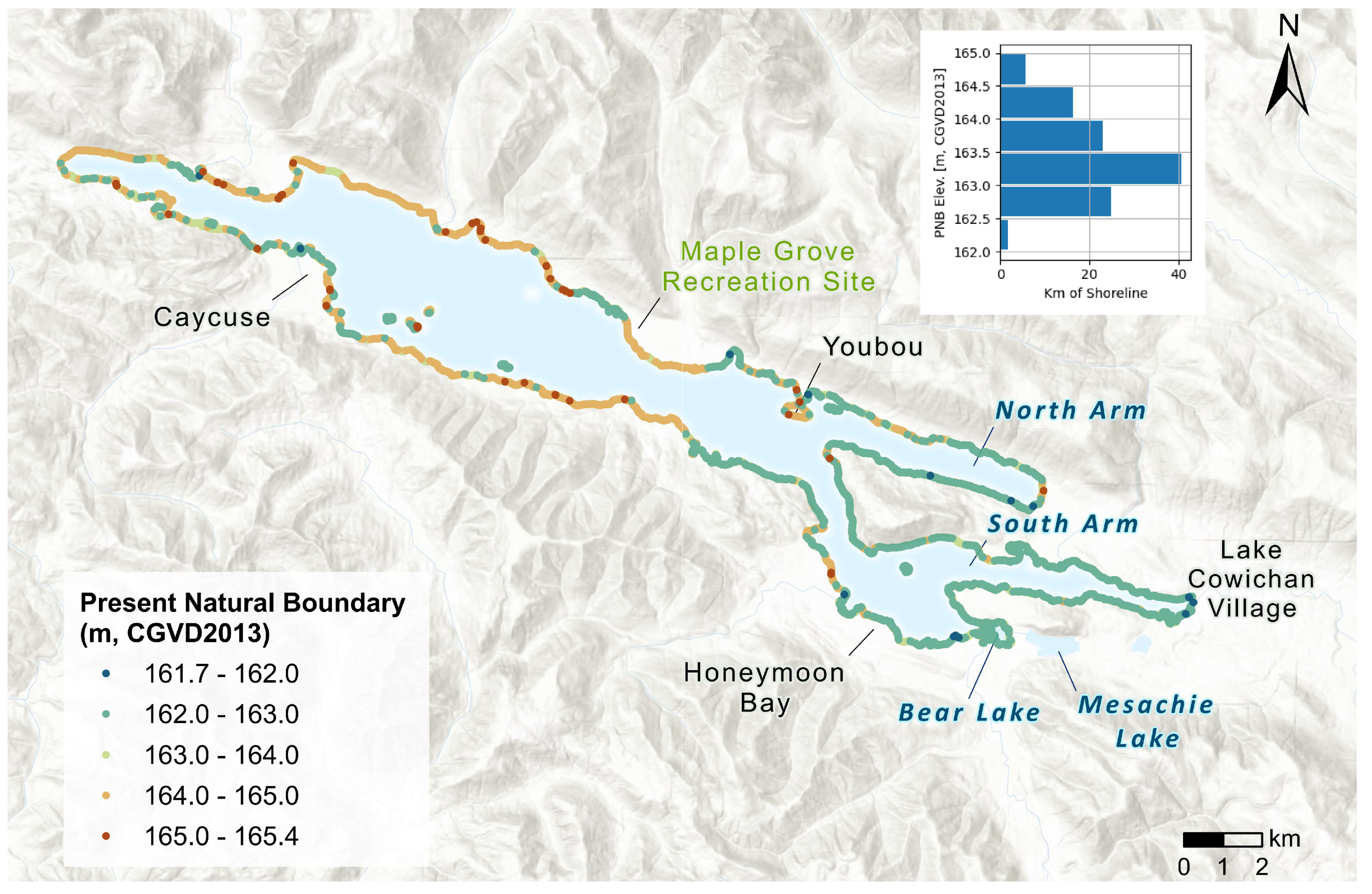
The survey points, along with detailed topography and orthophotos, were used in a desktop study to estimate the natural boundary location around the lake and islands. The elevation was then interpolated onto the PNB line from the DEM. The resulting dataset has an approximate along-shore spacing of 5 m. The elevation of the present natural boundary around Lake Cowichan is shown in
Figure 2. There is a considerable range in the elevations, from 161.7 m to 165.4 m.
4.1.4. Sediment and Vegetation
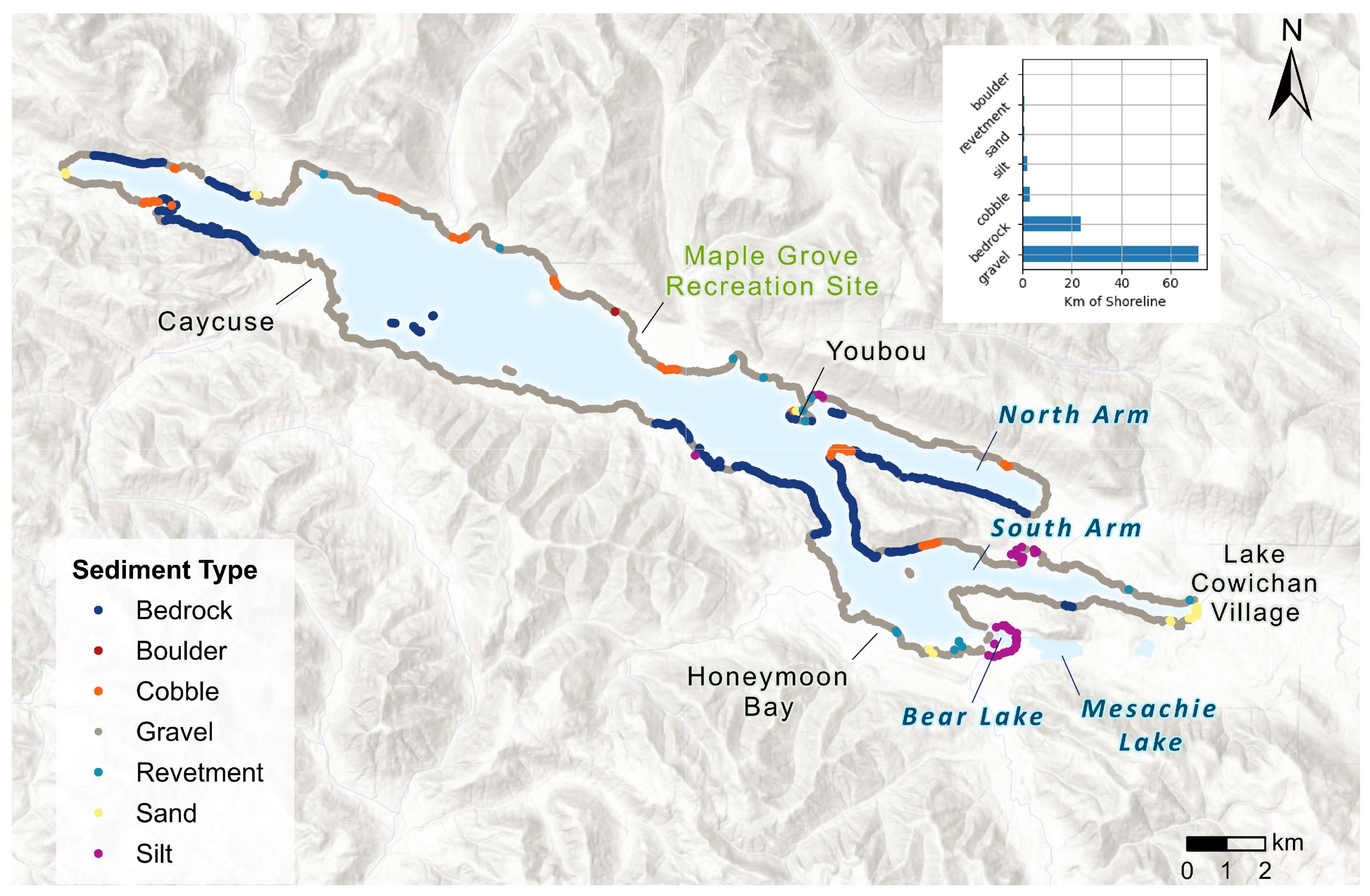
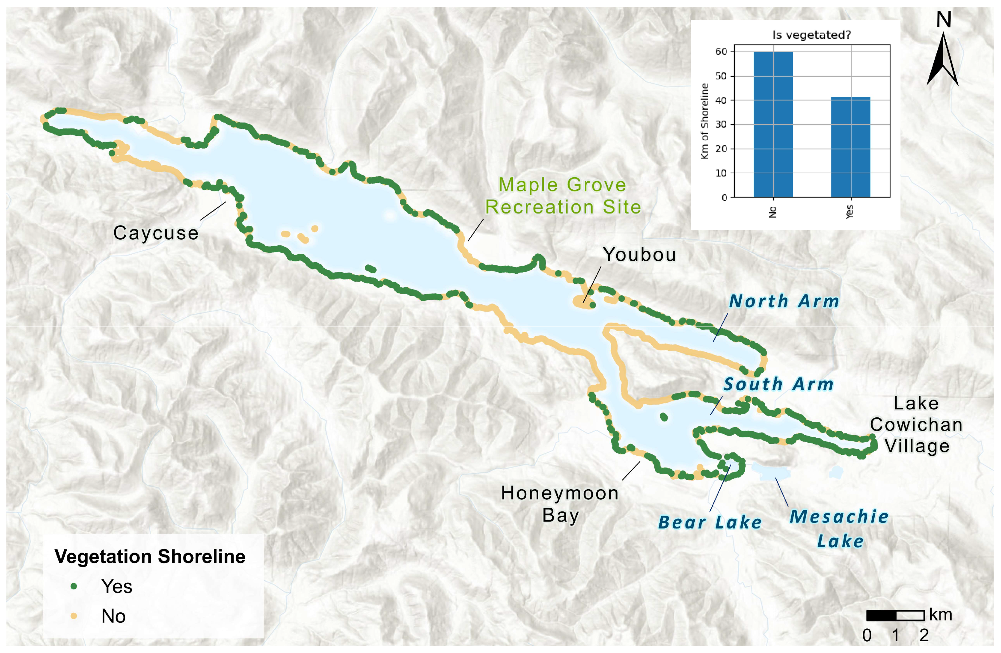
The shoreline band above the water line at the time of the field assessment (El. 162.27 m) was visually classified and mapped based on the sediment type and the presence of vegetation. Sediment was classified into the following Wentworth grain size categories: boulder (>256 mm), cobble (64–256 mm), gravel (2–64 mm), sand (0.063–2 mm), and silt (<0.063 mm). Additional shoreline classes of bedrock and revetment (e.g., walls, riprap, groynes, etc.) were also delineated.
The classification of the sediment around Lake Cowichan is shown in
Figure 3. The inset of
Figure 3 provides a histogram of sediment classes. The presence of vegetation at the 162.27 m contour around Lake Cowichan is shown in
Figure 4. The inset of
Figure 4 provides a histogram of the presence of vegetation.
4.1.5. Winds, Waves, and Water Levels
Two small weather buoys were deployed from February to September 2021. The buoys recorded wave and wind conditions, and were deployed in the south arm and near Youbou. For the purposes of comparison with modelled wind speeds, the observations were scaled from 1 to 10 m using a log profile and a friction factor of 0.01.
Daily observations of lake levels, river levels, and river flow rate at the Cowichan Lake Weir were obtained from the Canadian Water Survey for the period of 1952 to 2021 inclusive.
4.2. Computational Models
4.2.1. Water Level Model
Though an excellent record of lake levels is available at the Cowichan Weir, it was necessary to develop a water level model to estimate water level conditions with the implementation of the proposed weir upgrades. A model was developed which simulates the lake water level and river discharge using a water balance calculation with daily time-step:
where
is the lake level at timestep
i,
is the average net-inflow rate,
is the average outflow rate,
is the duration of the time step, and
is the surface area of the lake at the current water level.
Net inflows to the lake over the historic record were inferred based on the observed incremental change in lake water levels and river discharge. A rating curve for the upgraded weir system was developed by Stantec [
15] using hydrodynamic simulations of the weir, gates, and adjacent watercourses. The control logic for the upgraded weir system was developed by Stantec with guiding input from the Cowichan Water Use Plan [
16].
Using this new rating curve and control logic, along with the inferred inflows, the lake water levels resulting from the weir upgrades were estimated.
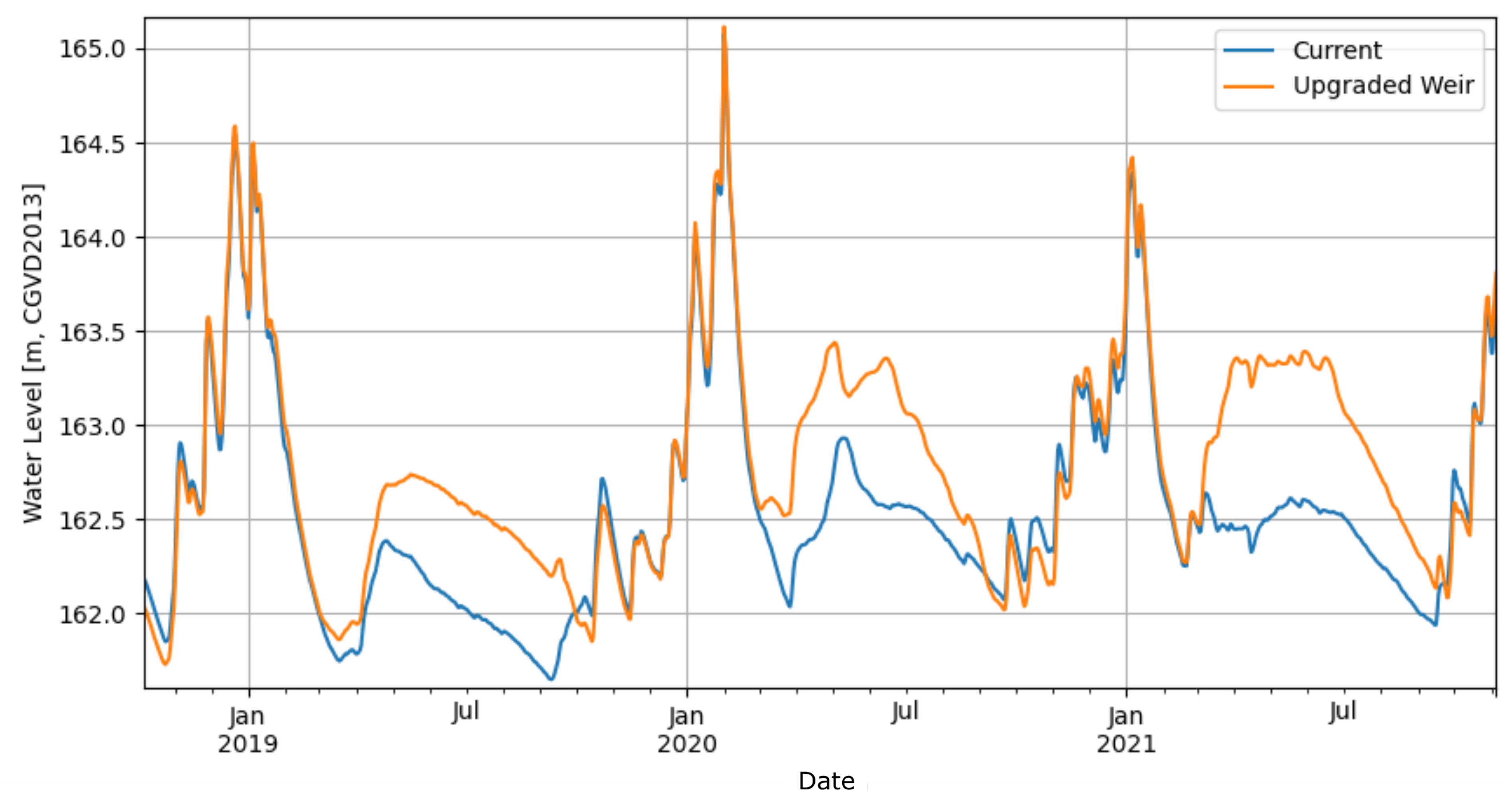
Figure 5 shows an example time series of lake level for the existing and upgraded weir. The model was used to estimate lake levels with the weir upgrades over the period from 1981 to 2021.
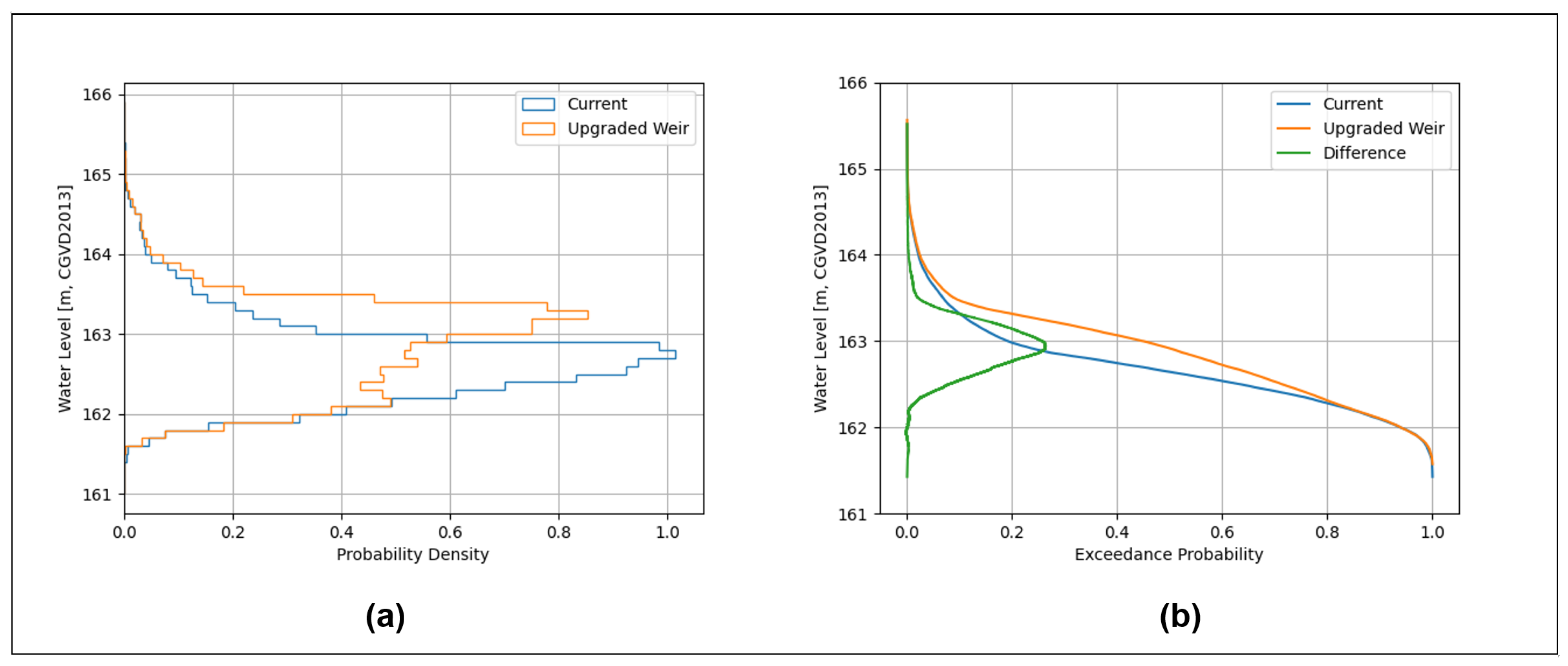
Figure 6 shows the (a) probability density curves and (b) the exceedance probability curves for current conditions and for the proposed raised weir. As designed, the proposed raised weir will store more water in the lake during spring, increasing availability for discharge during the dry summer months. The proposed raised weir has little impact on lake levels during the fall and winter. In both scenarios, water levels typically range from 161 to 165 m. The difference in average lake levels between historic and proposed weir conditions is 18 cm.
4.2.2. Wind and Wave Models
To estimate the wave climate of Cowichan Lake, a high-resolution spectral wave model was developed based on the SWAN wave modelling software v41.31 [
17]. An unstructured computational grid was used, with resolution varying from 100 m in deep water to 5 m at the shoreline. The model was run in stationary mode with sequential simulations at one hour time steps.
Initially the wave model was forced by 2.5 km wind fields from Environment and Climate Change Canada’s High Resolution Deterministic Prediction System (HRDPS) [
18,
19]. However, it was found that the wind fields and resulting wave estimates did not agree well with observations from the weather buoys. The mountainous topography surrounding the lake significantly affects local wind conditions. The HRDPS model, even with 2.5 km resolution, is not sufficiently resolved to capture the details of the local wind fields. This was most pronounced with winds blowing perpendicular to the axis of the lake, when the HRDPS wind estimates tend to be much larger than those observed on the lake surface.
To better capture the details of the local fields, the HRDPS model was down-scaled to about 100 m using the WindNinja Software v3.7.1 [
20]. WindNinja is developed by the Missoula Fire Sciences Laboratory for the US Department of Agriculture and is primarily used to support wildfire management operations in wild, mountainous terrain. The model was run in stationary mode, using a domain-averaged wind boundary condition, and using the conservation of mass and momentum solver (which uses a specialized version of the OpenFOAM [
21] solver in the background). WindNinja was run for a range of wind speed and direction boundary conditions and the results were assembled into a response matrix. The time series of wind fields was recovered by using the domain-averaged HRDPS wind velocity series to interpolate the response matrix.
The wave model results using the down-scaled wind fields show much better agreement with observations from the two weather buoys (see
Figure 7 for locations).
Table 1 shows the model evaluation statistics for significant wave height (
). At both buoys the root-mean-square
and bias (
B) in
is low, as is the Pearson correlation coefficient (
R). This indicates that, on average, the model error is low, but that the model lacks skill in deterministically estimating the
. However, for both buoys, the slope of the quantile–quantile plot (
) is close to 1.0, indicating that the model is skillful at estimating the statistical distribution of
. This is in line with qualitative observations that, because of limited fetch, wave conditions change rapidly on the lake with small changes in wind direction and speed, making deterministic estimates more challenging than the typical coastal environment.
The wave model was used to estimate wave conditions over the lake for the period of 2017 to 2021 (the period for which HRDPS data is available). Two different runs were executed. The first run (hind-cast) was for historic conditions, with water level boundary conditions specified based on the observed conditions. The second run (future-cast) was for the same period, with the only difference being that the water levels were specified assuming that the weir upgrades were in place through that period.
Figure 7 shows the average wave power (AWP) over Cowichan Lake for the hind-cast run. AWP is calculated as:
where
is the wave power transport in W/m for the
ith hour in the dataset, and
N is the total number of hours. As expected, because of the limited fetch, the south arm of the lake has low wave power compared to the rest of the lake. Wave power is higher in areas with larger fetch, in the northern portion of the lake (northwest of Youbou), where there is significant fetch from both the NW and SE.
To facilitate regression analysis with the other shoreline variables, it was necessary to calculate the shoreline incident AWP at each reach. First, the parametric wave results were interpolated onto the shoreline transect nodes. Then, at each time step, the wave conditions along each transect node were evaluated sequentially, starting offshore. The wave conditions at the node closest to shore, but before depth induced wave breaking, were selected to represent the shoreline incident wave conditions. This resulted in a single time series of wave conditions for each transect throughout the modelling period.
To better represent the possible range of wave power and water level combinations, the wave hind-cast was re-sampled over the period 1981–2021. Bootstrap re-sampling with replacement was carried out in monthly blocks. Selections from the source datasets were made randomly +/− one month. For example, in the re-sampled dataset, January 1981 might be filled with any of the December, January, or February months from the source dataset. The same re-sampling was used for both the hind-cast and future-cast datasets.
5. Analysis
5.1. Hydrologic Climate
5.1.1. Historic Conditions
Peak and mean wind speeds, as well as water levels, tend to be larger in the winter months compared to the summer. However, there are important differences in the characteristics of each season.
During winter, winds are driven primarily by large-scale weather systems propagating through the region. This season is characterized by frequent storms, with peak wind speeds up to about 15 m/s, wave heights up to about 0.6 m, and lasting up to several days. Lull periods between storms, where wind speeds are below 5 m/s and waves are small, may last days to weeks. The direction of the largest wind speeds tends to align with the northwest and southeast axes of the of the lake. Winds blowing perpendicular to the axis of the lake tend to be lower in magnitude due to the sheltering effect of the surrounding mountains. Lake levels are highest in this season due to significant precipitation, which primarily falls as rain at lower elevations. The control gates are fully open during this season and the weir is overtopping.
Through the spring, the frequency and magnitude of strong large-scale weather systems decline, and the influence of thermally driven sea-breezes increases. On the east coast of Vancouver Island and Cowichan Lake, the sea breeze is usually from the easterly direction. The sea breeze typically peaks around 6 m/s, producing significant wave heights of up to about 0.25 m on Cowichan Lake. Precipitation through the spring is variable year-to-year, with some years much drier than others. Water level control is initiated in the spring (1 April) to retain run-off from snow-melt at higher elevations. Regulation holds water levels relatively constant from April to June.
During the summer, strong large-scale weather systems are infrequent, so sea breeze tends to be the dominant driver of wind conditions. When the sea breeze is dominant, lull conditions typically last only the night-time hours. Inflows to the lake through run-off and precipitation are small through this season, and it is primarily lake storage that maintains river base-flows. Because of this, the lake level declines at approximately 1 cm per day. In very dry years, the water level may fall below the weir crest, necessitating the pumping of water over the weir to maintain river base-flows.
In the fall season, the occurrences of sea-breeze diminish, and wind conditions quickly transition to be dominated by large-scale weather systems, similar to the climate experienced through the winter months. However, on average, wind speeds are somewhat lower than in the winter months. With the onset of the rainy season, the lake storage will begin to recharge. The onset of rains is variable and may begin anywhere from early September to late October.
Vessel wakes were quantified by MarineLabs, using published techniques [
22,
23], based on time-series measurements from the two weather buoys. It was found that, on average, vessel wakes accounted for less than 5% of the overall wave energy. Consequently, vessel wakes were not included in this analysis.
5.1.2. Changes with Weir Upgrades
The proposed weir upgrades will raise the weir by 70 cm and initiate regulation earlier in the spring (1 March). Because the control gates are open in the winter, the lake levels during this period will not change substantially. During the spring, the water levels will hold the lake level at a higher elevation for longer. During the summer, water levels will decline at a similar rate; however, because the levels at the start of the season are higher, the levels by the end of the season will not be as low. Lake levels through the fall will be slightly higher because of the higher starting condition.
The change in average wave power with the weir upgrades are small throughout most of the body of the lake but are larger closer to shore. The difference in AWP close to the shoreline between the scenarios is typically less than 5% but is up to 30% in some cases, and in both the positive and negative direction. For example, in sheltered areas, the average wave power can decrease, as deeper water reduces the tendency of refraction to bend waves towards some sections of the shoreline. Wave power can increase in areas with shallow foreshores which break larger waves and dissipate energy under current conditions but do so to a lesser extent with increased lake levels.
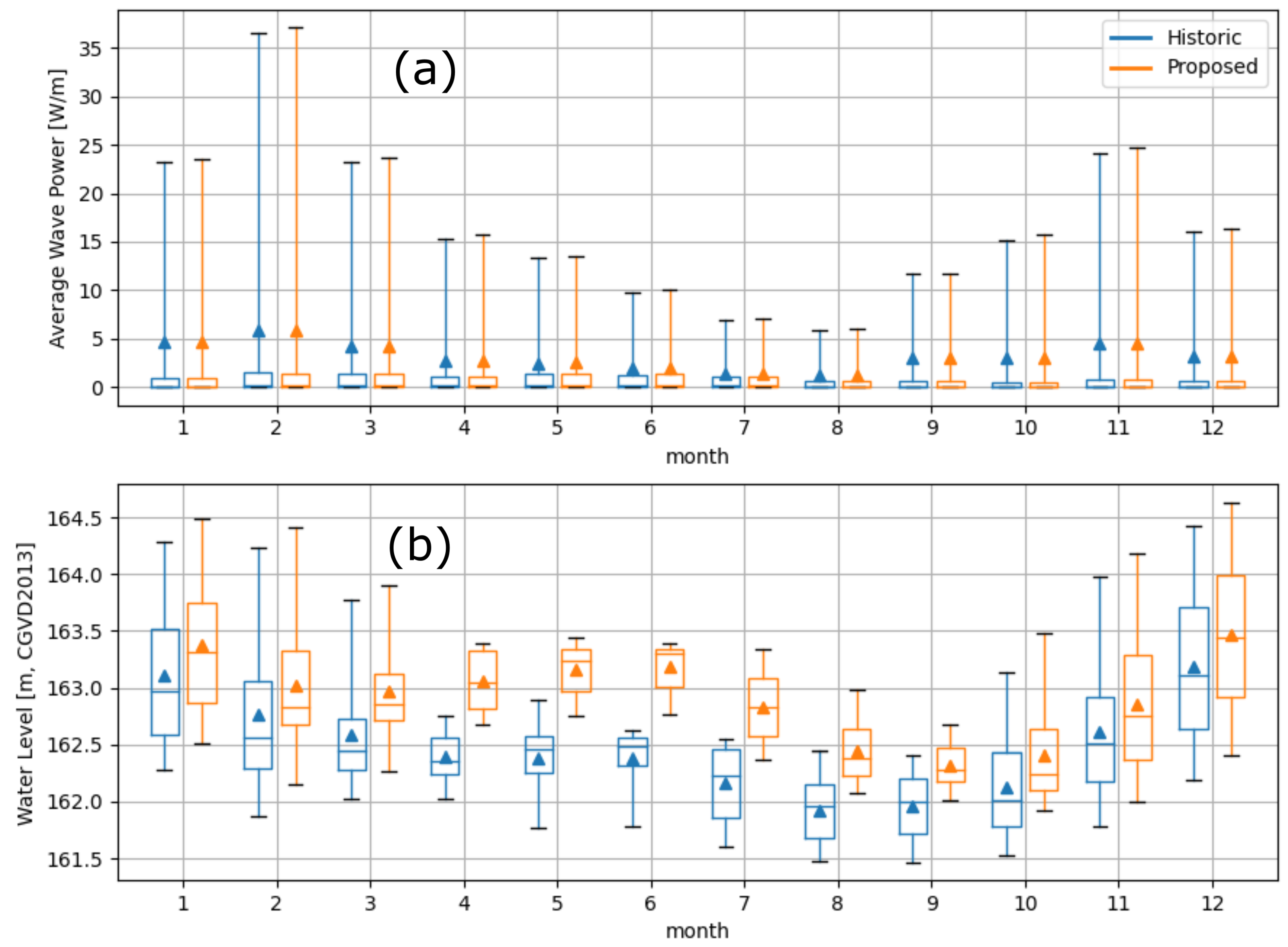
The monthly boxplots in
Figure 8 provide detail on how the average wave power (AWP) and water levels probability distributions change throughout the year.
Figure 8a represents shoreline incident AWP near the Maple Grove Recreation Site. At this location there is very little difference in AWP for historic and proposed weir conditions. Of note is that, except for the summer, the mean value of AWP is considerably higher than the 75th quantile. This indicates that a significant portion of the overall wave energy is from infrequently occurring events. The bulk of the wave energy occurs in the fall and winter months.
Figure 8b indicates that the main change in lake levels with the raised weir occurs during the spring and summer regulation period. The range of water levels in the late summer is also reduced in the late summer due to the increased effectiveness of the regulation. There is a small increase in winter water levels as well, but the difference in the most extreme events is very small (<10 cm).
5.2. Variability of the Natural Boundary Elevation
This analysis takes the atypical approach of quantifying the natural boundary in terms of its elevation, rather than the more common surveying approach of using its location in a 2D plan. This selection was made because it facilitates quantitative comparison to other morphological or hydrological variables. However, before proceeding, the suitability of the elevation metric was assessed.
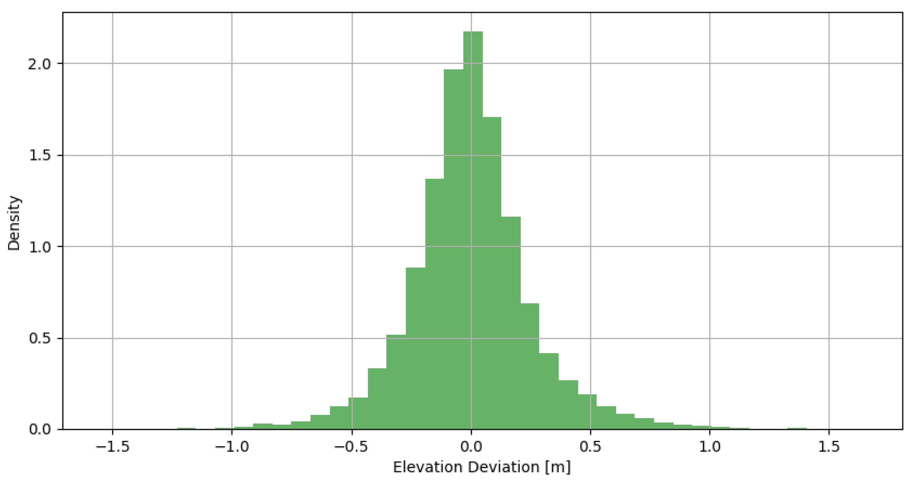
The natural boundary was quantified at 5 m alongshore resolution, while the other variables were quantified for each 50 m reach. This provides the opportunity to assess the intra-reach variability of the present natural boundary elevation. The deviation of the PNB elevation within each reach from the reach-mean was aggregated over all reaches, and plotted as a PDF in
Figure 9. The standard derivation is 0.25 m and the 90% confidence interval ranges from −0.40 to 0.42.
Figure 9 illustrates the significant variability of PNB elevation, even within a 50 m reach. This variability is thought to be the result of several factors, both real and resulting from data collection and processing approaches. Real factors include the true variability of the PNB elevation over short distances, while data collection and processing factors include the subjectiveness of identifying the natural boundary location, the density of surveyed PNB locations, and the associated interpolation of the PNB location and conversion of the interpolated location into an elevation using the DEM. The reach-mean PNB elevation (
) was selected as the PNB location metric for this study because the objective of the study was to develop a best estimate of PNB change around the lake perimeter and, therefore, it is thought that the average value over the reach is more representative of the PNB elevation than the value at, for example, a spot location on the transect.
5.3. Regression Analysis
Statistical analysis was used to uncover the relationship between the hydrologic variables (waves, beach slope, sediment, vegetation) and the PNB elevation. The data from the 2021 reaches provided the basis for this analysis. The influence of the water level itself on the natural boundary elevation could not be tested because the water level is essentially constant over the lake.
Linear regression analysis was applied between each of the hydrologic variables and . The results indicate that 27% of the variance in can be attributed to AWP, with values below 3% for the other variables. The use of higher quantiles of wave power were explored in the regression analysis, but showed no improvement in explaining the variance in .
Multiple linear regression analysis with AWP, sediment type, and presence of vegetation as independent variables increased the
variance explained to just 28%. Further, sediment type becomes statistically insignificant, and vegetation type nearly so. This indicates that, of the variables tested, AWP is by far the most significant predictor of
. It should be acknowledged that AWP is responsible for 27% of the
variance and the other 73% remains unaccounted for. There are many potential causes of this difference in variance, including the assumption of linearity, uncertainties in the
estimates (
Section 5.2), uncertainties in the AWP estimates (
Section 4.2.2), human influence on
(disturbance), and the use of AWP as the sole parameter to represent the wave climate (e.g., the influence of extreme events are not explicitly considered).
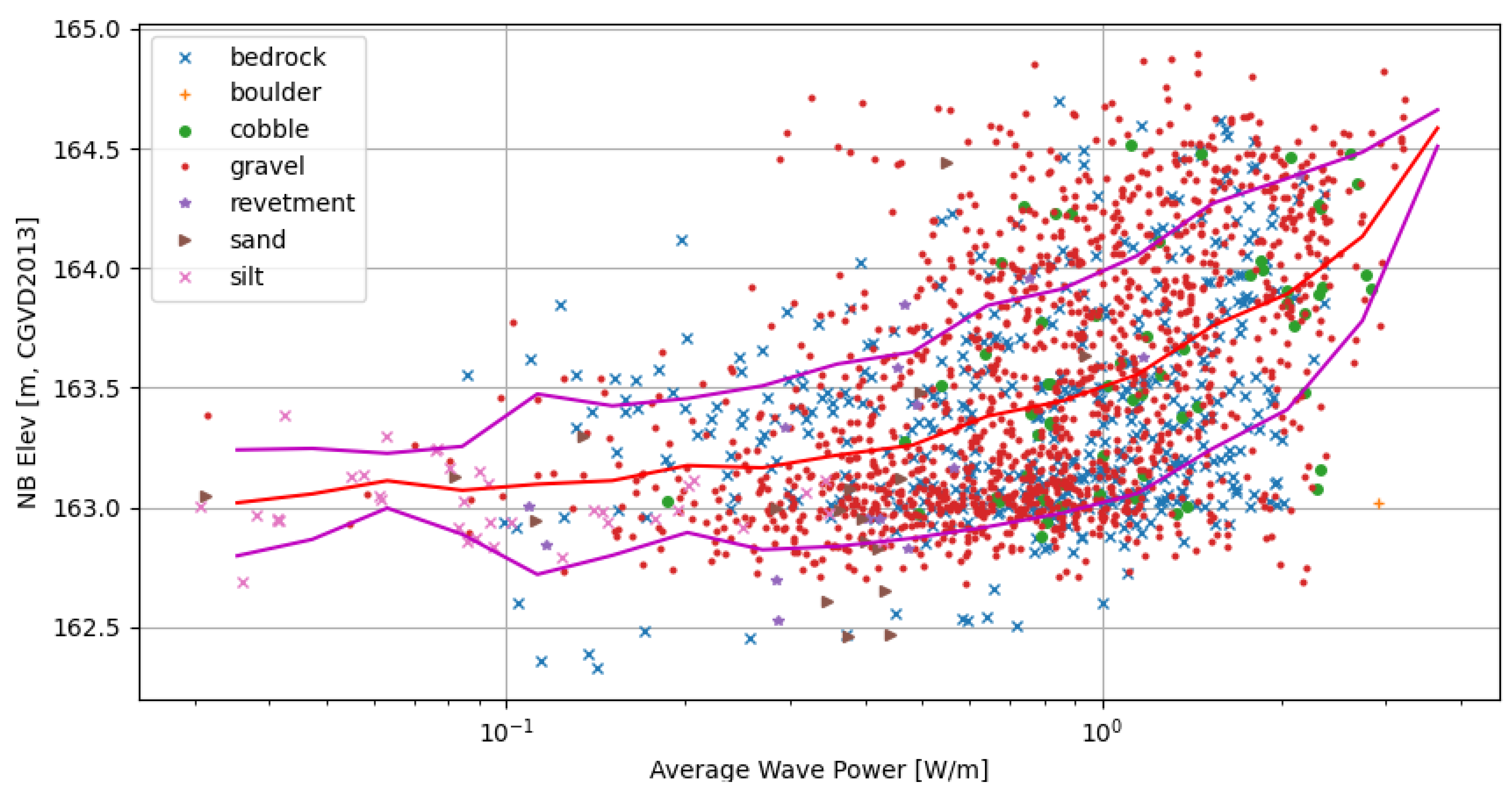
Figure 10 illustrates the relationship between
and AWP on a log scale, with the marker colour and shape indicating sediment types. In this plot, each marker represents a different shoreline reach. As suggested by the regression analysis, the binned-mean trend shows that an increase in AWP corresponds with an expected increase in
; however that increase is not linear. Below about 0.4 w/m of AWP, the trend line is almost flat, suggesting that, below this threshold, AWP has little influence on PNB elevation. This makes sense when considering the definition of the natural boundary from
Section 3: for low wave energy areas the natural boundary is likely primarily a function of the presence of water, rather than the action of water.
As suggested by the regression analysis, limited correlation can be discerned in the distribution of sediment types with PNB elevation. It is clear that silt only exists where wave power is very low, and that gravel is the most predominant sediment type. There is some indication in
Figure 10 that the PNB elevation of bedrock reaches tends to be lower than the average trend. This is backed up by some specific in-field observations of bedrock-adjacent sand or gravel beaches, where the difference in PNB elevation was over a metre. However, the scatter is large and, in general, the relationship between the sediment type and the PNB elevation is unclear.
While a clear relationship between AWP and PNB elevation has been demonstrated, a satisfactory explicit equation for PNB elevation could not be developed based on the data available. The variability in the natural boundary elevation appears to play a large role in this challenge, but uncertainty in the hydrologic data or an incomplete or over-simplified representation of morphologic characteristics may also play a role.
5.4. Estimating Natural Boundary Change
5.4.1. Hypothesis Refinement
The regression analysis indicates that, of the variables considered, wave conditions have the most influence on . However, the relationship between AWP and remains unclear. This section uses the results of the regression analysis and physical arguments to refine the original hypothesis
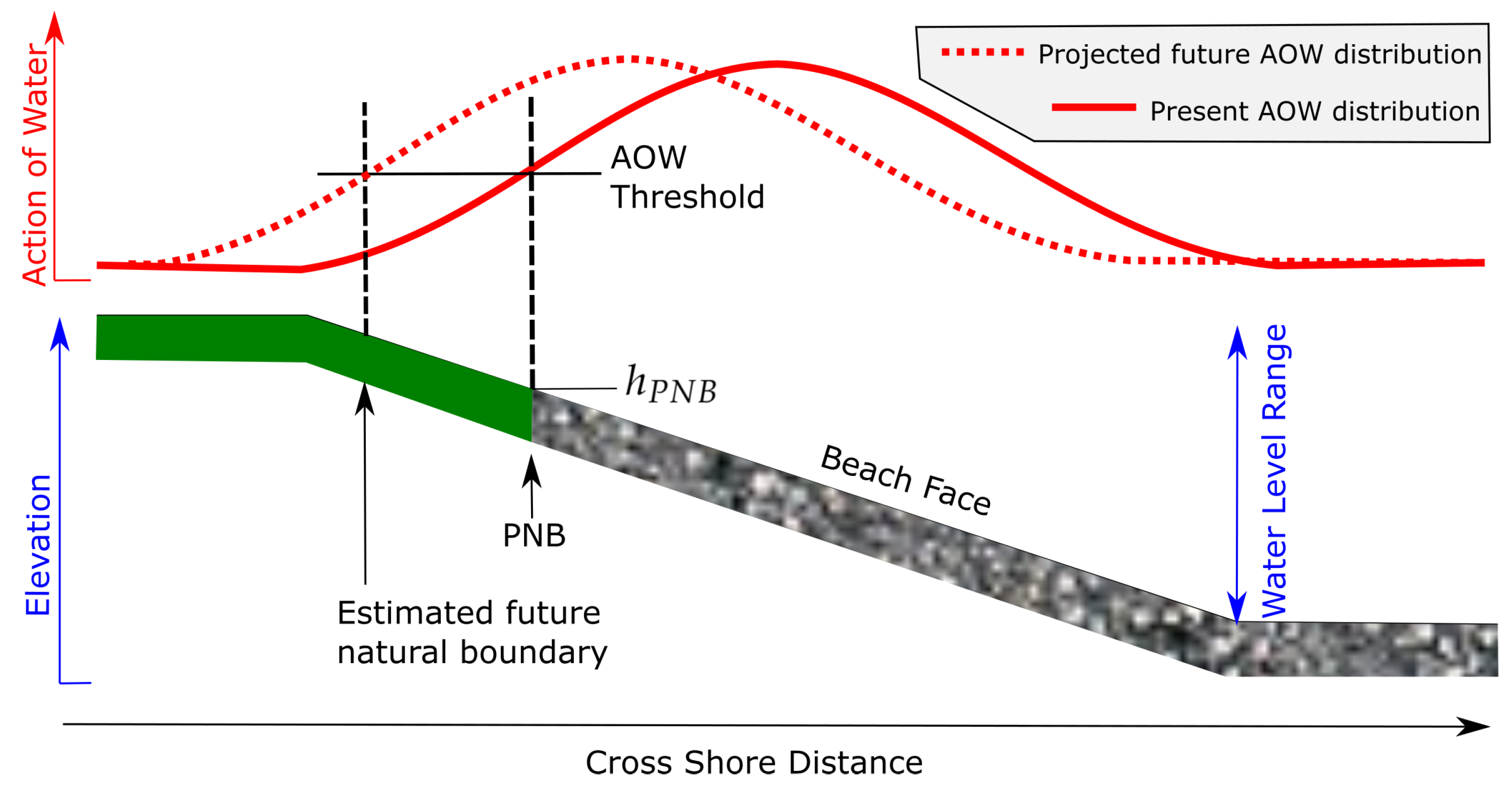
In low wave energy environments, it may be assumed that is dictated by the presence of water alone, as indicated by a transition from aquatic to terrestrial vegetation. However, in higher wave energy environments we expect to be a function of both the presence of water and the action of water. Generally, waves can only act on that portion of the shoreline that the swash can reach There are specific conditions, such as undercutting where this may not be true, but no evidence of substantial undercutting was observed at Cowichan Lake in our field work. Water levels can significantly modulate the portion of the shoreline that waves are able to act on.
The action of water (AOW) may be conceived as the dissipation of wave energy, wave-induced bottom stress, or another similar metric. In the multi-year averaged sense, the AOW varies in the cross-shore direction, with a peak somewhere near the mean of the water level range and tapering to zero at the maximum landward extent of wave swash. Below the PNB, the AOW is large enough to remove organics and fines to render the beach face essentially sterile; above the PNB, the opposite is true. So, the AOW at the PNB must represent a threshold for that particular shoreline. If the hydrologic climate changes and the threshold value of the AOW migrates up or down the beach face, then we would expect a corresponding change in
and PNB location.
Figure 11 illustrates this concept in a schematic.
The AOW threshold may be used to estimate changes in , however implicit in the calculation is the use of the . In doing so, information about the inherent shoreline character and resilience is included in the estimate of natural boundary change. For example, if we have a shore that experiences a high AOW, but has a relatively low , we conclude that this shoreline is particularly resilient to the AOW. This may be because of the shoreline slope, the sediment type, the local vegetation, or because the shore experiences few external disturbances (animals, humans, surface runoff, sedimentation, pollution, etc). Even with changes to the prevailing wave or water level regime, we would expect that the shoreline character and associated resilience would remain similar in the future.
5.4.2. A Parametric Approach
Proposed here is a simple approach where the AOW is quantified as the AWP when water levels are above the PNB elevation. This metric (
) is calculated as:
where
is the water level at hour
i, and the relation in square brackets indicates that the sum is conditional on the water level being greater than the natural boundary elevation.
A similar relation was developed for reaches with low wave energy (AWP < 0.4 W/m), where the natural boundary is presumed to be primarily dictated by the presence of water. With this approach, an inundation threshold is calculated based on the water level exceedance probability at the natural boundary elevation, .
This parametric approach has the advantage of efficient computations and that detailed wave runup modelling is not required. However, this approach lumps together all AOW occurring above the PNB, neglecting the details of how AWP is distributed on the beach profile. This assumption is likely acceptable where is close to the high end of the water level range, because waves occurring with water levels above will generally be acting on the same section of beach face. However, this assumption may break down when is relatively low compared to the range in , because the range in water levels above is so large, that at different times the waves could be acting on different sections of the beach face.
5.4.3. A Modelling Approach
While the parametric approach is efficient, it neglects the fact that the AOW on the shoreline will be distributed over the beach face in a non-uniform manner depending on the beach slope, wave conditions and, lake level.
A modelling-based approach was developed using the XBeach wave hydrodynamics and morphodynamics modelling software v1.23 [
24]. This approach aims to overcome some of the simplifications of the parametric approach by explicitly modelling the AOW on the beach face.
The XBeach software was configured as in
Table 2. The non-hydrostatic simulation option is computationally expensive but is required in this application, because the waves and shoreline on Cowichan Lake are such that swash action occurs primarily at the frequency of the incident waves, not as surfbeat. The morphodynamic and groundwater modules of XBeach were not used in this analysis.
For the purpose of this analysis, the AOW along the beach slope was quantified as the mean plus one standard deviation of bottom shear stress (). Bottom stress is the force per unit area acting over the beach face, which tends to cause movement of sediment, and erosion. Using the standard deviation as well as the mean recognizes that the natural boundary is affected by, not just the net stress, but also the oscillating component, which will tend to suspend fines and organics. Contrary to the parametric approach, the AOW threshold was identified at the natural boundary location, rather than the sum of the AOW above .
Each transect was set up as a one-dimensional XBeach model. A suite of model runs was defined for a range of significant wave height () and water level input conditions. For each transect peak wave period, () was defined as a function of . Each run used a different model grid, where the grid resolution in the swash zone was approximately 2.5 cm, increasing up to 50 cm on the outer boundary. Each run was executed for one hour of simulated time. The model results were interpolated based on the shoreline incident significant wave height and water level to recover a time series of bottom stress along the beach slope at one-hour timesteps. The time series was then averaged and smoothed to produce a characteristic distribution of the AOW along the beach face. This procedure was executed for both the existing and upgraded-weir wave and water level datasets.
6. Results and Discussion
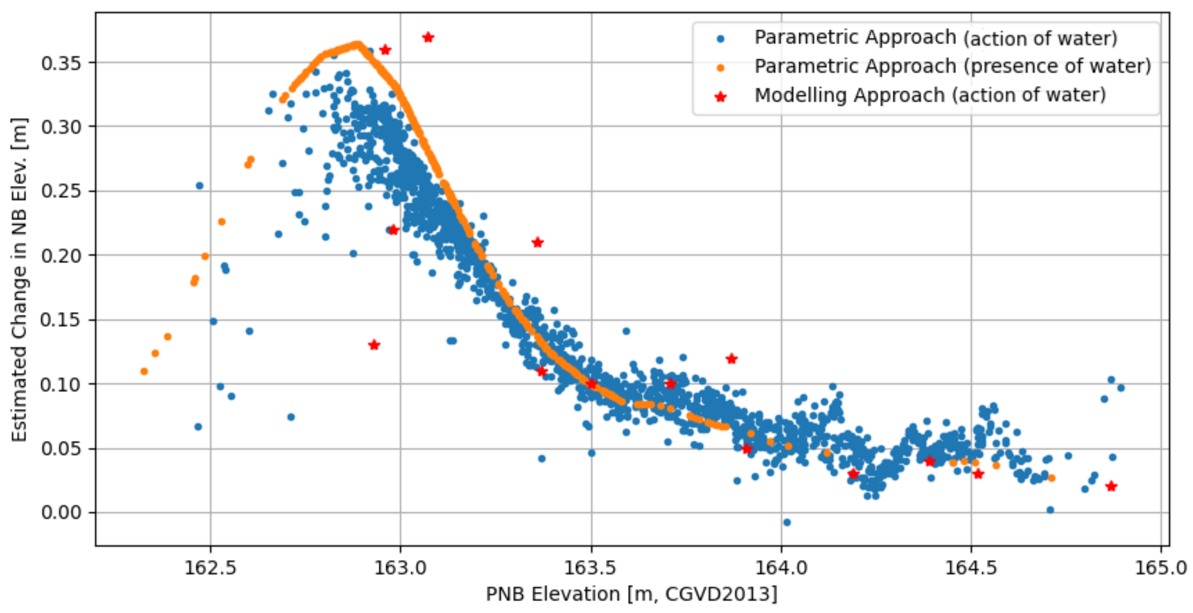
In this Section, the projected change in water levels with the proposed weir upgrades at Cowichan Lake are used to test and inter-compare the parametric and modelling-based approaches for estimating natural boundary elevation change (), proposed in the previous section.
First, the parametric method was used to estimate
for all reaches. The action of water approach was used on all reaches where
W/m, and the presence of water approach was used for transects with lower AWP. The resulting estimates are shown as blue dots (water action) and orange dots (presence of water) in
Figure 12. The maximum estimated
is about 0.4 m and occurs for PNB elevations of 162.9 m. This coincides with the largest shift in lake level occurrences associated with the proposed raised weir (refer to
Figure 6).
The results illustrated in
Figure 12 indicate much greater variability in
than the change in average water levels (18 cm) would imply. This variation occurs because the method depends not on water levels directly, but primarily on the change in inundation frequency (or exceedance probability) at the PNB. Due to the raised weir, water levels are higher in the spring and summer period (about 163.1 m compared to 162.5 m). This is reflected in the water level exceedance probability and difference curves in
Figure 6b. Reaches where
is in this range will be more frequently inundated with the proposed weir upgrades, and it is estimated that the natural boundary will migrate upwards. The magnitude of that migration (
) depends on the change in inundation probability.
The estimates using the parametric approach based on the action of water and the presence of water differ, as one would expect. Because lake levels are the same at all reaches, the estimated based on the presence of water follow a continuous curve with . The wave climate, on the other hand, changes from reach to reach, so there is scatter in the curve. Both methods follow a similar trend because both depend on the how often the PNB is inundated. The estimates are larger for the presence of water approach for PNB elevations near 162.9 m. This is because there is a weak positive correlation between and AWP, so that at lower there is less change in between the scenarios than the change in inundation frequency alone would suggest.
The modelling approach was applied to fourteen reaches with
W/m and a range of
. The number of reaches was limited by computational cost. The
estimates for all fourteen transects are summarized in
Table 3. The parameter
is the mean bottom stress plus one standard deviation, and
is the modelled value at
. Through the modelling, it was found that the oscillating component was dominant over the mean component, typically by an order of magnitude or more.
If all reaches were characterized by similar sediment and vegetation, then one would expect the value of to be similar between reaches. The results of the modelling indicate that the value of varies considerably between each reach, but most are in the order of Pa. Those reaches with a relatively high and low AWP, such as reach M-854 and M-1900, tend to have a lower . This may indicate that the PNB at these locations is controlled by a few wave events which coincide with high water levels. For the remainder of the reaches, the value of is within an order of magnitude. This would appear to be a plausible range given the likely differences in sediment and vegetation between the reaches, and the inherent uncertainties is the assessment.
The modelling results are plotted against the statistical estimates in
Figure 12. In general, the
estimates agree well between the two methods. There is a mean difference of −1 cm, a root-mean-square difference of 8 cm, and a mean absolute difference of 5 cm. It is notable that the largest differences are found for transects with relatively low average wave energy. This difference is expected because at lower
the water action above the natural boundary will be spread over a relatively large swath of beach, some of which will not impact the location of the PNB. The modelling approach captures this nuance, but the parametric approach does not.
Despite these issues, given the many differences in the assessment methods and the approximations and assumptions inherent in each method, the results are similar, providing some confidence that they are reasonable. In-field testing is required to further test the refined hypothesis and to evaluate the appropriateness of the proposed methods.
7. Conclusions
This paper explores the relationship between the natural boundary and the hydrologic and morphologic climate on a large lake. Based on the analysis of extensive data from Cowichan Lake, Canada, it is hypothesised that the present natural boundary elevation is related to the average action of water (waves) occurring when water levels are at or above the natural boundary elevation.
Two process-based methods for estimating natural boundary change are proposed based on this hypothesis. As the authors were unable to identify any pre-existing methods for estimating natural boundary change, the methods developed here are preliminary, requiring significant simplifications and assumptions. Without field data for validation, the methods are verified through inter-comparison of results.
The natural boundary is usually determined on the ground through survey. To facilitate quantitative analysis in this study, the natural boundary was parametrized in terms of its elevation. On average, the present natural boundary elevation was found to have a standard deviation of 0.25 m within each 50 m of shoreline reach. To reduce this variability, the reach-average present natural boundary was used for quantitative analysis.
Linear regression analysis of the available data show insignificant correlation between the variables beach slope, sediment type, and presence of vegetation with natural boundary elevation. However, there were some specific in-field observations of bedrock-adjacent sand or gravel beaches, where the difference in PNB elevation was over a metre. Significant correlation was found between average wave power and natural boundary elevation. Below 0.4 W/m of average wave power the correlation with natural boundary elevation is very weak, suggesting a transition from dominance of the action of water (waves) to the presence of water.
This research was not able to develop a satisfactory method for explicitly estimating natural boundary elevation. Instead, physical arguments, supported by data were used to develop two implicit methods for estimating natural boundary change, one based on the observed statistical relationship between the shoreline morphology, the hydrologic climate and the natural boundary elevation, and another method based on detailed analytical modelling of the bottom stress from shore-incident waves. These methods are both based on the concept that a threshold of the action of water acts at the present natural boundary, and that a shift in the location of that threshold will result in a corresponding shift in the location of the natural boundary.
The parametric and modelling methods suggest similar levels of natural boundary change with the proposed raising of the weir at Cowichan Lake, though there is significant scatter. The agreement is best for reaches with high present natural boundary elevation, and degrades for reaches with lower elevations. This is likely due to simplifications in the parametric approach, which start to break down at lower elevations.
The modelling approach requires significant preparation effort by a qualified professional and is computationally expensive, so is problematic for practical application at a large scale. Both methods are limited by the requirement of a survey of the existing natural boundary and the practical difficulties of performing a natural boundary survey of a large shoreline.
This work could be improved by reducing the uncertainty in some of the input datasets. While the natural boundary dataset used in this analysis was extensive, it relied on interpolating elevation from a limited number of point survey locations from a DEM. The DEM was based primarily on LiDAR measurements, which had relatively high uncertainty in areas of dense vegetation. It may be possible to reduce this variability through in-situ surveying of the PNB elevation at all reaches; however, this is practically difficult for large shorelines, and where trees obstruct GPS signal at the natural boundary.
The wind fields used to drive the wave hind-cast were limited in their ability to deterministically reproduce the winds observed at Cowichan Lake. It may be possible to improve the wave hind-cast through the adoption of new, more sophisticated wind hind-cast models as they become available.
Planned upgrades to the Cowichan Lake weir will affect the water level regime. This planned change presents a unique opportunity to monitor the response of the natural boundary location to changing hydrologic conditions. Future work is planned to collect this data and to quantitatively evaluate the performance of the discussed methods for estimating natural boundary change. In addition to the existing lake and river level monitoring stations, future monitoring should include shoreline weather conditions (including wind) and wave measurements with sufficient fidelity to detect and quantify boat waves. Following weir upgrades, the natural boundary elevation should be surveyed annually at a selection of locations around the lake until it is observed to stabilize.


