1. Introduction
Dissolved oxygen (DO) plays a pivotal role in water environmental science, serving as a critical indicator of the health and sustainability of aquatic ecosystems [
1,
2,
3,
4]. Oxygen dissolved in water is essential for the survival and growth of aquatic life, including fish, invertebrates, bacteria, and plants [
5,
6]. Maintaining a healthy balance of DO is essential, as both excessive and inadequate levels can pose severe risks to the ecosystem [
7]. High concentrations of DO can lead to the excessive growth of an organism, thereby disrupting the ecosystem balance [
8]. Conversely, low DO levels can result in hypoxic conditions that jeopardize aquatic life [
9]. Predicting DO concentrations facilitates the management and conservation of aquatic resources, aids in the planning and operation of water treatment processes [
10], and helps in the timely detection and mitigation of potential environmental risks [
11]. A precise prediction model can offer valuable insights into the future state of the ecosystem, thus providing a powerful tool for decision makers in crafting effective strategies for water resource management and pollution control [
12]. Despite its significance, the accurate prediction of DO levels remains a challenging task due to the complexity of aquatic ecosystems, the multifaceted interactions between numerous influencing factors, and the spatiotemporal variability in DO levels [
13].
Existing methods for predicting DO concentrations can generally be classified into three categories: physical models, statistical models, and data-driven models [
14]. Physical models are developed based on the physical laws governing DO dynamics, such as the Streeter–Phelps model [
15]. These models utilize differential equations to represent the oxygen balance in water, taking into account factors, like biochemical oxygen demand, reaeration, photosynthesis, and respiration [
16]. While these models are theoretically sound, they often require a multitude of precise measurements and fail to account for the complex interactions among various environmental factors, making their application, in practice, quite challenging [
17,
18]. Statistical models, such as regression models, time-series analysis, and Box–Jenkins models, have also been applied to DO prediction [
19,
20]. These models rely heavily on historical data, and their success depends on the inherent linear relationships among variables [
21,
22]. However, the interactions between different environmental factors influencing DO levels are complex and often non-linear, which restricts the accuracy and applicability of these models [
23,
24,
25]. Data-driven models, including machine learning and deep learning models, have gained popularity in recent years owing to their capability to capture complex non-linear relationships and their adaptability to various situations [
26,
27,
28]. These models, such as artificial neural networks [
29,
30], support vector machines [
31,
32], and random forest models [
33,
34], have shown promising results in DO prediction. However, most existing data-driven models consider only temporal dependencies, overlooking the spatial interactions among different locations, which can lead to suboptimal prediction performance [
13,
35,
36,
37].
To mitigate the limitations of traditional models and incorporate spatial dependencies, recent studies have turned to hybrid models, such as Convolutional Neural Networks (CNNs) combined with Long Short-Term Memory (LSTM) networks [
38,
39,
40]. CNNs, renowned for their success in image processing tasks, are used to capture spatial correlations by considering the area of interest as an image-like structure [
41,
42,
43]. Meanwhile, LSTMs handle the temporal dependencies due to their unique architecture that can learn and remember over long sequences [
44], alleviating issues encountered with traditional recurrent neural networks, like vanishing or exploding gradients [
45].
However, these models present their own set of constraints [
46]. Firstly, they usually assume a Euclidean space to capture spatial dependencies [
47], which might not accurately reflect the geographical and topological properties of the real-world scenarios, where different meteorological stations and bodies of water exhibit non-Euclidean relationships. Secondly, the heterogeneity of data [
48], which is often a combination of structured and unstructured data (like temperature, wind speed, etc.) [
49], presents a challenge. Existing models may not fully capture the complex correlations between these different types of data [
50]. Moreover, the architecture of these models is rigid, which can hinder the comprehensive incorporation of multiple meteorological factors [
51]. These factors, such as temperature, pressure, dew point, wind direction, wind speed, and precipitation, have intricate and non-linear impacts on DO dynamics [
52]. For instance, the fixed kernel sizes in CNNs are not conducive to capturing these varying influences and interactions [
53], leading to insufficient consideration of environmental factors and, thus, inaccurate predictions.
In light of these limitations, there is a need for a more flexible and sophisticated modeling approach. This approach should accommodate the complex, non-linear interactions among various factors in non-Euclidean spaces and consider both temporal and spatial dependencies simultaneously. This underpins the primary motivation of our study.
The realization of such a sophisticated modeling approach calls for the exploration of advanced data representation and learning techniques. Recently, two techniques have shown exceptional promise in various domains for handling data with complex dependencies and non-Euclidean structures: Graph Embedding techniques [
54] and the Transformer model [
55]. Graph Embedding techniques have the potential to capture non-Euclidean spatial dependencies effectively [
56]. By transforming the nodes of a graph into a continuous vector space while preserving the structural information of the original graph [
57], these techniques facilitate the understanding of complex inter-node relationships and topological properties. They have been successfully applied in several domains, including social network analysis [
58], bioinformatics [
59], and recommendation systems [
60], yielding significant improvements over traditional methods. On the other hand, the Transformer model, a deep learning model primarily designed for natural language processing tasks [
61], presents a powerful tool for temporal dependency modeling. Its unique self-attention mechanism can effectively capture long-range dependencies in time-series data by weighing the influence of different time steps based on their relevancy [
62].
In response to these challenges and opportunities, we propose a novel, sophisticated model for accurate DO concentration predictions that effectively leverages the spatial and temporal dependencies present in multiple meteorological factors across various meteorological stations. Our approach comprises the following: a Meteorological Graph Construction module, wherein meteorological stations are treated as graph nodes; a Geospatial Graph Convolutional Embedding module, applying Graph Convolutional Networks and a Multilayer Perceptron to obtain a comprehensive feature vector; a Feature Encoding and Temporal Concatenation module for feature refining and sequence formation; and, finally, a Temporal Transformer Prediction module, which uses the Transformer’s self-attention mechanism for capturing long-term dependencies in data. Our proposed model, tested and validated on real-world data, significantly outperforms existing models, effectively demonstrating its utility in handling the complex, non-linear interactions in DO concentration predictions. We anticipate that this work will contribute to environmental science by improving our understanding of DO dynamics and advancing the predictive modeling techniques in the field.
2. Materials
2.1. Study Area
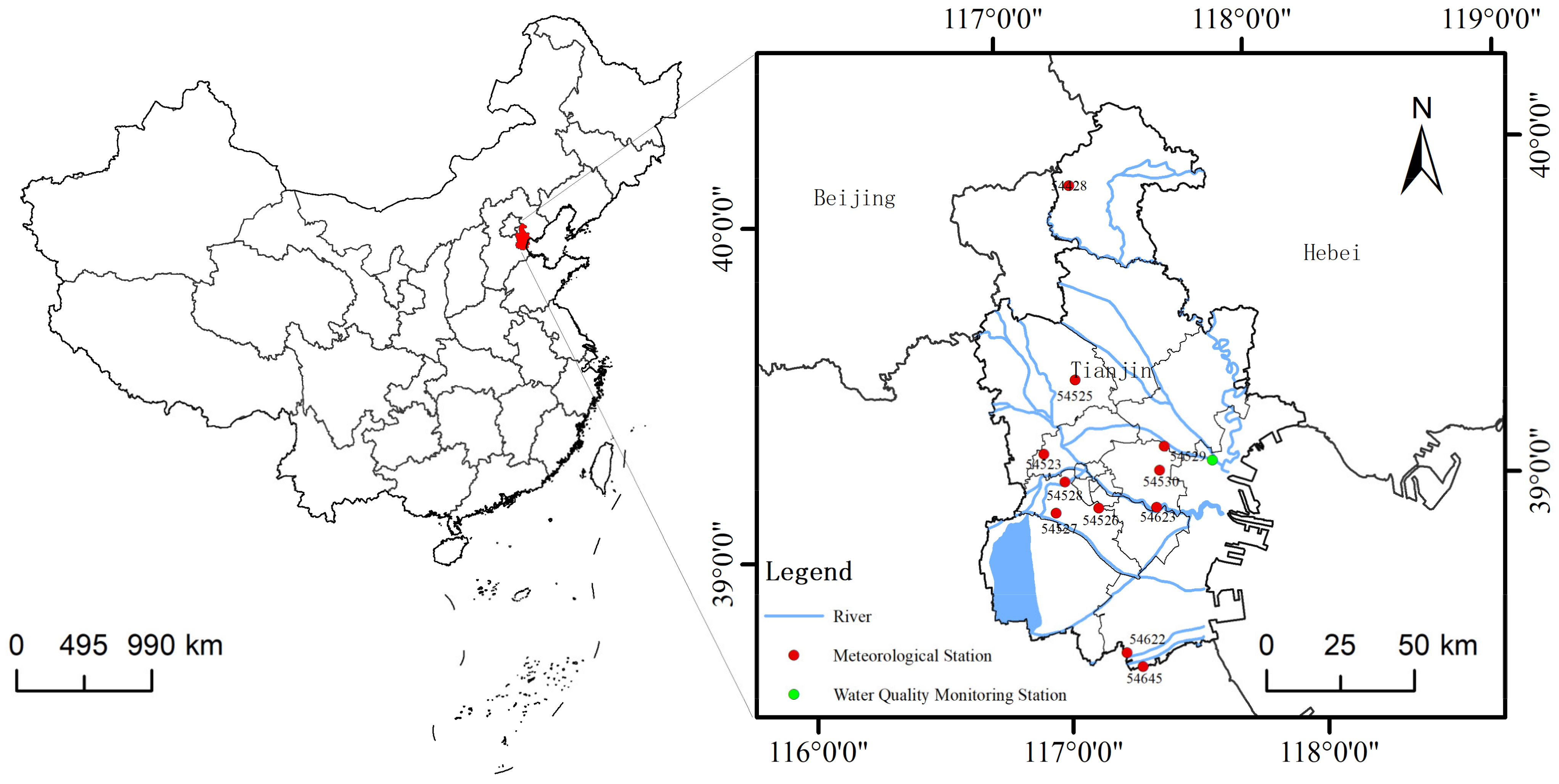
The focus of this investigation is the city of Tianjin, located in the eastern coastal region of North China, approximately 120 km southeast of the capital, Beijing. Encompassing an expansive geographic expanse exceeding 11,300 square kilometers, Tianjin offers a diverse backdrop for studying various meteorological patterns and their impacts on water quality parameters.
Positioned uniquely, Tianjin experiences a humid continental climate influenced by monsoon winds. This climatic influence results in distinct seasonal variations—hot, rainy summers juxtaposed with cold, dry winters. Such seasonality, especially the heavy rainfall during the summer season, significantly influences the region’s water bodies. The intricate interrelationship between meteorological factors and the hydrological characteristics of Tianjin’s aquatic systems generates a complex environment for the study and prediction of the dissolved oxygen concentrations in these bodies of water. Tianjin boasts a network of diverse water bodies, including rivers, canals, and lakes, interconnected through the prominent Haihe River that empties into the Bohai Sea. Notably, our research pays particular attention to the Binhai New Area, specifically focusing on the Ji Canal Tide Gate within the Haihe River Basin. Given the considerable influence of both natural and human-induced activities on the Ji Canal Tide Gate, it represents a suitable site for examining the typical water quality challenges in the region.
The urbanized nature of Tianjin city, together with its distinct hydrogeological features, introduces multifaceted aspects to its water quality parameters. Our focus, the dissolved oxygen concentrations—a crucial determinant of aquatic health—is impacted by an array of factors. These factors span meteorological elements, including temperature, atmospheric pressure, and wind dynamics, as well as precipitation levels. Moreover, these influencing factors exhibit considerable spatial and temporal variability across Tianjin’s vast geography.
Through this investigation, we aim to elucidate the intertwined dynamics between meteorological conditions and water quality, particularly the dissolved oxygen concentrations. This study intends to enhance the predictability of dissolved oxygen levels in Tianjin’s water bodies. We anticipate that the insights gleaned from this research will contribute to the academic discourse on water quality prediction and pave the way for more informed, sustainable water resource management practices in Tianjin, aligning with both its ecological imperatives and urban development objectives.
Figure 1 illustrates the distribution of the research area and the locations of the data collection sites.
2.2. Data Source and Collection
The objectives of this research necessitate the collection of detailed and well-documented datasets from diverse sources. For this study, the data were aggregated from two primary sources: the China National Environmental Monitoring Center (CNEMC) and the United States National Climatic Data Center (NCDC).
The CNEMC, a respected repository of environmental data in China, provides the critical water quality parameter—dissolved oxygen concentrations. The data were systematically harvested from the CNEMC’s official online portal (
https://szzdjc.cnemc.cn/, accessed on 8 February 2023). The period of data collection extended from 1 January 2021 to 31 December 2022. The data were registered with a temporal resolution of four hours, affording a detailed perspective on the dynamics of dissolved oxygen concentrations over the chosen period. The water quality monitoring station employed for gathering dissolved oxygen concentration data is situated in the Binhai New Area within the Ji Canal Tide Gate of the Haihe River basin, with geographical coordinates of 117.7274° E, 39.1185° N.
On the other hand, meteorological data were sourced from the NCDC (
https://www.ncei.noaa.gov/, accessed on 17 April 2023), a preeminent institution within the purview of the National Oceanic and Atmospheric Administration (NOAA), USA. This research incorporated a spectrum of meteorological parameters, including temperature, pressure, dew point, wind direction and speed, and precipitation. Contrasting with the water quality data, meteorological data were captured at a temporal resolution of three hours, thereby yielding a more granular understanding of the atmospheric conditions. The acquisition of meteorological data adhered to the same timeframe as the dissolved oxygen data. Notably, the data from 2021 served as a foundation for subsequent model training, while the 2022 dataset was reserved for model validation and testing. These datasets, combined, will help in building a robust and accurate predictive model, addressing the complex interplay between water quality and meteorological parameters.
The geographical distribution of the monitoring stations is extensively detailed in
Table 1, specifying the monitoring areas, longitude, latitude, sensor altitude, and station altitude for each station.
Table 1 offers a detailed view of the distribution of monitoring stations across the research region, with longitude and latitude allowing for precise geographical coordination. The altitudes provide an indication of the vertical profile of the station locations, which may influence certain meteorological and environmental factors. Further,
Table 2 provides the specifics of the collected parameters, their respective physical meanings, and their units.
Table 2 elucidates the physical meanings of the parameters, offering a comprehensive view of their significance in environmental studies. The designated instruments ensure precise data collection, crucial for subsequent data analysis and model development.
2.3. Data Preprocessing
Data preprocessing is a pivotal component in our study, as it ascertains the completeness, consistency, and accuracy of our dataset, thereby ensuring the credibility and robustness of our model predictions.
Our dataset is gathered from two primary sources: meteorological stations and water quality monitoring stations in Tianjin. However, due to various issues, such as equipment failure, station maintenance, and technical complications, the raw dataset might contain missing and outlier values. To counter the potential negative impacts these factors could exert on our analysis results, we implemented a two-step procedure:
Elimination of missing values: Initially, we discarded records containing missing values that could occur due to issues, like equipment malfunction, station maintenance, or other technical problems. This ensures the completeness of our dataset, enhancing the accuracy of our analysis.
Removal of outliers: Subsequently, we excluded outlier values from the dataset, i.e., readings significantly deviating from the normal range. Such readings could occur due to equipment malfunction or transient, non-representative environmental conditions. This step aids in reducing data noise and enhances the accuracy of the model’s predictions.
Upon cleaning the data, we encountered a crucial issue: aligning data with different time resolutions. Specifically, our meteorological data were recorded every three hours, while water quality parameters (i.e., dissolved oxygen concentrations) were recorded every four hours.
To address this, we adopted a straightforward yet effective method: resampling. We sampled the data every 12 h. This not only solved the inconsistency in time resolution but also made our data more manageable. For the water quality parameters, sampling every 12 h meant that we had two samples each day. Over the span of two years, this would yield approximately 1460 (365 days/year × 2 years × 2 samples/day) samples. The meteorological factors were treated similarly, sampled every 12 h.
Through this, we could directly associate the meteorological conditions at each timestamp with the corresponding dissolved oxygen concentrations. Furthermore, through resampling, we preserved the essential information, allowing us to account for temporal variations in meteorological conditions impacting the dissolved oxygen concentrations. This preprocessing step, hence, resolved the inconsistency in time resolution and enriched our data, providing a more comprehensive and detailed input for subsequent analysis and model prediction.
3. Methodology
3.1. Overview of the Model Architecture
Building predictive models to anticipate changes in critical ecological parameters, such as dissolved oxygen concentrations, is a significant challenge in environmental science and engineering. Addressing this complex task requires processing heterogeneous data sources and accounting for spatial and temporal correlations between these data points.
In this study, we propose a comprehensive model architecture that integrates data from eleven meteorological stations spread across Tianjin City. These stations provide a wealth of meteorological information, including temperature, pressure, dew point, wind direction, wind speed, and precipitation. Our aim is to predict the dissolved oxygen concentrations in the “Production Circle Gate” section of the Tianjin Southern District.
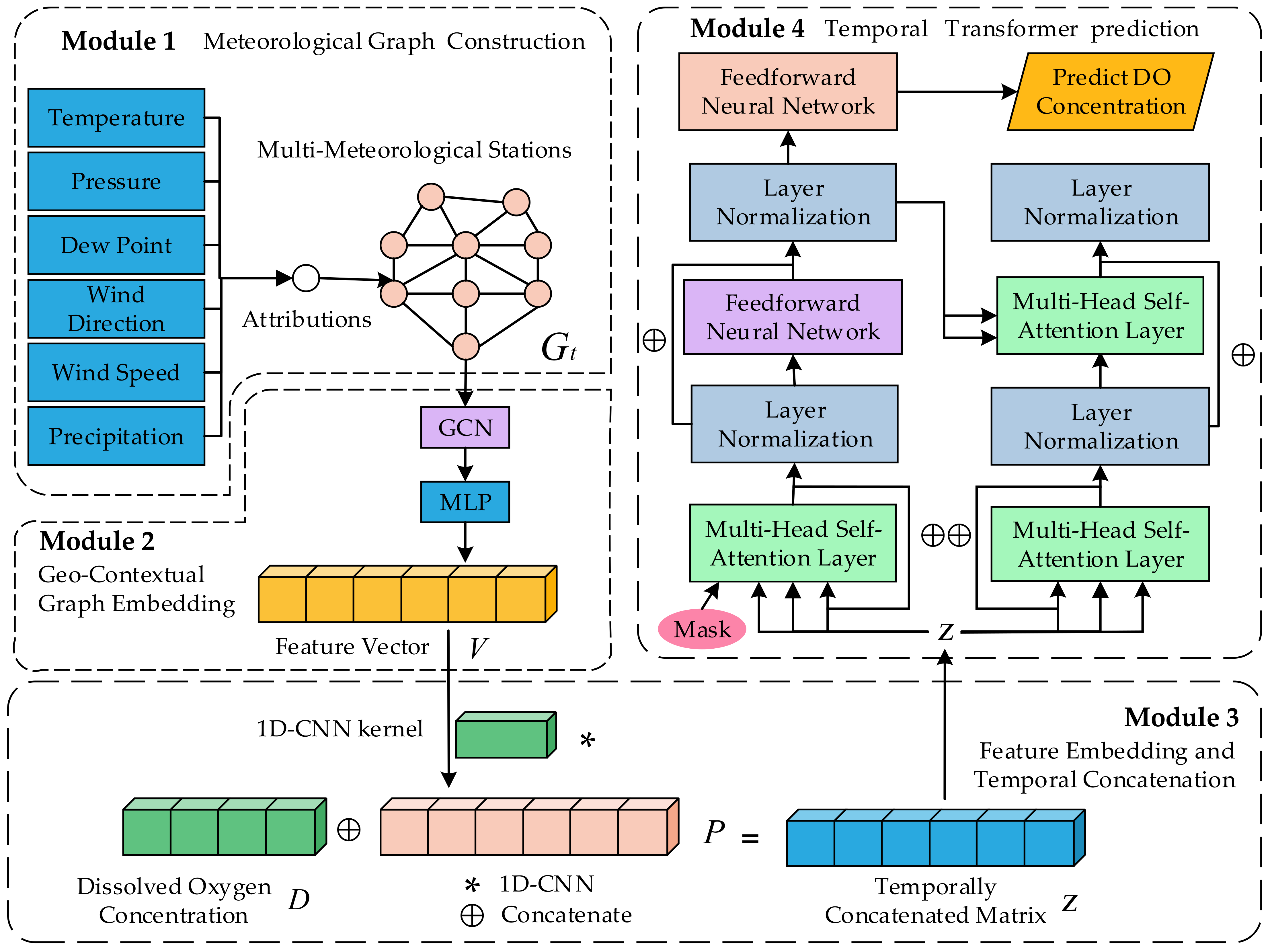
Figure 2 presents the entire framework of the model, providing a comprehensive overview of its structure and components.
In our modeling, the subscript notation denotes the time window that starts with and ends at , encompassing meteorological data from multiple stations and dissolved oxygen concentrations for analysis. Specifically, we denote the time series of meteorological factors for each station , where corresponds to the number of meteorological stations, as . Here, refers to the current time step, and , which defaults to 5 in this study, defines the temporal window size. Furthermore, represents the historical dissolved oxygen levels at the “Production Circle Gate” section during the same time window. The primary objective of our model is to predict the future dissolved oxygen levels at time , denoted by .
Our model’s design is composed of a layered architecture, systematically processing the data through a sequence of sequential operations represented by the composite function:
This function captures the hierarchical nature of our model concisely. Here, represents the Geo-Contextual Graph Embedding Module. It processes the time-series meteorological factors from the different stations and generates a unified feature vector that encapsulates the spatiotemporal characteristics and correlations of these stations. The function denotes the Feature Encoding and Temporal Concatenation Module. It encodes the feature vector output from the Graph Embedding Module along with the historical dissolved oxygen data at the target site into a temporally concatenated feature vector. Finally, the function corresponds to the Temporal Transformer Prediction Module. The combined feature vector is input into a Transformer model to predict future dissolved oxygen levels at time .
By structuring our model into these modularized steps, we can account for the complex spatiotemporal dynamics inherent in the meteorological and dissolved oxygen data. The following sections provide a more detailed discussion of the inner workings and motivations behind each module:
Meteorological Graph Construction Module: This module forms the foundation of our methodology. It capitalizes on the graph-based representation of the meteorological data, enabling us to capture the spatial configuration of meteorological stations and the intricate relations between their respective data.
Geo-Contextual Graph Embedding Module: As the heart of our model, this module provides a sophisticated mechanism for transforming the raw meteorological data into a meaningful representation. It utilizes the power of Graph Convolutional Networks to process and compress the high-dimensional meteorological data into a lower-dimensional feature vector, capturing both local and global patterns.
Feature Encoding and Temporal Concatenation Module: This module acts as a bridge between the Geo-Contextual Graph Embedding Module and the Temporal Transformer Prediction Module. It prepares the model’s input data by encoding the meteorological feature vector and combining it with the historical dissolved oxygen data, creating a richly informative input for the final prediction module.
Temporal Transformer Prediction Module: This module is the terminal point of our model architecture. It leverages the potent capabilities of Transformer models in handling sequential data and makes the final prediction of dissolved oxygen concentrations, providing valuable insights for environmental management and policymaking.
Through the intricate combination of graph-based representation, convolutional processing, and transformer-based prediction, our model offers a pioneering approach to predicting dissolved oxygen concentrations using meteorological data. The proposed model is designed to cope with the inherent challenges of environmental data, namely its high dimensionality, complex dependencies, and spatiotemporal variability. With its robust architecture and advanced components, our model stands as a promising tool for environmental monitoring and management.
3.2. Meteorological Graph Construction Module
To harness the inherent spatial and temporal correlation between various meteorological stations and effectively feed these into our model, we opt for a Graph Neural Network (GNN)-based representation. GNNs offer a promising approach to capture non-Euclidean characteristics, thereby overcoming the limitations of traditional Convolutional Neural Networks (CNNs) that are primarily designed for Euclidean or grid-like data. Moreover, GNNs are highly capable of embedding heterogeneous data types, which is particularly advantageous given our diverse set of meteorological factors across multiple stations.
Within this framework, each meteorological station is represented as a node in our graph, while the meteorological factors of each station serve as the node’s attributes. Let us denote by
the time series of meteorological factors for each station
, where
corresponds to the number of meteorological stations, and
denotes the time window under consideration. Then, the attribute tensor
for our graph can be formed as:
Furthermore, the connections between these nodes are determined based on the geographic proximity of the stations. Here, we represent these connections using an adjacency matrix . The matrix is an matrix, where indicates whether there is an edge between node and node .
The geographic proximity is calculated using the Haversine formula, which computes the distance
between two points,
and
, on the Earth’s surface:
where
is the average radius of the Earth, approximately 6371 km. A threshold of 85 km is then set. If the distance between two stations is less than or equal to this threshold, an edge is created between these two nodes (i.e.,
). Otherwise, no edge is formed (
). Formally, the adjacency matrix
is defined as follows:
The choice of an 85 km threshold was not made arbitrarily but was determined through extensive experimentation.
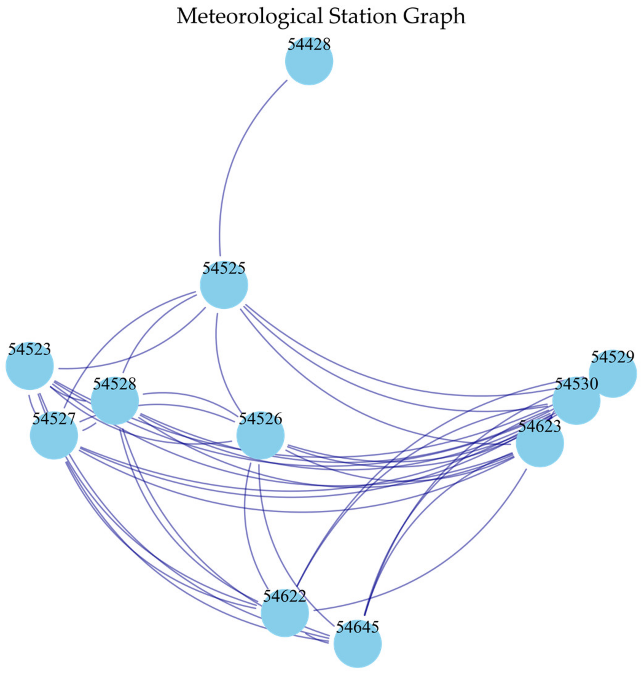
Figure 3 illustrates the connections between 11 meteorological stations under the optimal threshold condition of 85 km. In
Section 4, we present a detailed discussion on the selection of the threshold, highlighting how various options were evaluated to ensure the optimal representation of the spatial correlations between the meteorological stations.
With the construction of the adjacency matrix and attribute tensor, our model can efficiently exploit the spatial correlations among the meteorological stations. By leveraging the intrinsic benefits of graph-based representation, the proposed architecture caters to the complexities and nuances of environmental data, offering a sound basis for further stages of the model, including feature encoding and temporal prediction.
3.3. Geo-Contextual Graph Embedding Module
Graph embedding methods have garnered significant attention for their prowess in encoding nodes from a graph into a continuous vector space. This facilitates the deeper understanding of not only the graph structure but also the relationships and attributes between nodes. In this research, we specifically harness the power of the Graph Convolutional Network (GCN), a renowned variant of GNN methodologies. The GCN’s ability to integrate localized information from the graph structure proves integral in our study.
On the basis of the adjacency matrix and attribute tensor, as developed in
Section 3.2, we establish a graph representation
consisting of
nodes. These nodes embody meteorological stations, each possessing a set of specific meteorological attributes. The edges that connect these nodes are determined through geographical proximity and convey the relational network among the stations. The nodes within the graph
are symbolized by an attribute tensor
with dimensions
, where
represents the dimension of the meteorological factors at each individual station. The adjacency matrix of graph
, labelled as
, features dimensions
. In this matrix,
reflects the presence of an edge or connection between stations
and
.
Within the adopted GCN framework, a graph convolution operation can be mathematically denoted as follows:
In this equation, signifies the features of nodes at layer , with serving as the initial condition. acts as the weight matrix learned during the training phase at layer . is the degree matrix with , and acts as a non-linear activation function—in this research, the ReLU function.
The above operation signifies the dual process of feature transformation and neighborhood information aggregation. The newly transformed feature for each node amalgamates information from its immediate neighbors, providing a localised yet comprehensive summary of the node’s context within the graph. By performing this operation over multiple layers, we ensure the assimilation of a more extensive array of contextual information. The output derived from the GCN, denoted by , embeds crucial geographical and meteorological contexts for each meteorological station, thereby acting as a potent intermediate representation.
To further hone this intermediate representation, we introduce an additional transformation step facilitated by a Multilayer Perceptron (MLP). The MLP operates as a transformative function
that maps its input to a higher-dimensional feature space, thereby introducing non-linearity that is capable of capturing complex patterns within the data. The transformation operation of the MLP, which takes
from the last GCN layer as its input, is as follows:
where,
act as weight matrices,
denote bias vectors, and
represents an activation function. This configuration of the MLP facilitates the extraction of higher-level features from the graph embeddings, transforming the information into a more compact, information-rich representation. The resulting feature vector
encapsulates the output of the Geo-Contextual Graph Embedding Module, melding the geographical and meteorological context to provide a robust foundation for subsequent stages of our model.
In combining the GCN and MLP in this module, we effectively capture complex spatiotemporal patterns that are inherent in environmental data, significantly enhancing the representational power of the feature vector . Our Geo-Contextual Graph Embedding Module, through the adept combination of graph-structured data and multilayer neural networks, heralds a novel approach to processing spatiotemporal environmental data.
3.4. Feature Encoding and Temporal Concatenation Module
In this section, we delve into the Feature Encoding and Temporal Concatenation Module, a critical stage that bridges the graph-embedded meteorological features and the historical dissolved oxygen concentration measurements, laying the foundation for the subsequent Temporal Transformer Prediction Module. The Geo-Contextual Graph Embedding Module outputs a feature vector for each meteorological station, which is of dimension .
The first phase of this module entails the positional encoding of the feature vector
, employing a one-dimensional Convolutional Neural Network (1D-CNN). The process aims to uncover the latent spatial correlations within the meteorological features. For the feature vector
, the 1D-CNN applies a convolution operation, followed by a non-linear activation function; here, we consider the ReLU function. This can be represented mathematically as:
where
denotes the convolutional kernel,
is the bias,
represents the convolution operation, and
is the ReLU activation function. The output
is the positionally encoded feature vector of dimension
, where
is the dimension of the feature vector after CNN encoding.
The next step integrates the positionally encoded feature vectors with historical measurements of the dissolved oxygen concentrations. Let
be the historical dissolved oxygen concentrations from time
to
, which is of dimensions
. These historical measurements are appended to the positionally encoded feature vector
, forming a temporally concatenated matrix
of dimensions
:
where the brackets denote the concatenation operation, and the output
represents the temporally concatenated matrix.
The temporally concatenated matrix is a comprehensive time-series dataset that fuses the positionally encoded meteorological features with historical dissolved oxygen concentrations. The data are now prepared for the next module, the Temporal Transformer Prediction Module, that predicts the future dissolved oxygen concentrations. This Feature Encoding and Temporal Concatenation Module effectively brings together the meteorological data and dissolved oxygen history and instills a temporal facet to the model.
3.5. Temporal Transformer Prediction Module
The Temporal Transformer Prediction Module, drawing on the power of the Transformer model [
55], forms the heart of our proposed system, synthesizing the preceding stages’ outputs to predict future dissolved oxygen concentrations. The Transformer model’s pivotal strength, the self-attention mechanism, demonstrates proficiency in modeling both local and long-range dependencies in sequences, rendering it aptly suitable for our predictive task from the spatio-temporal environmental data. The Transformer architecture can be conceptually segregated into two primary components, the Encoder and Decoder, both of which are formed of multiple identical layers, each consisting of a self-attention mechanism and a position-wise feed-forward network.
The Encoder operates as a complex, sequential data interpreter. The input to the Encoder is the combined feature sequence , and its output is a high-dimensional representation of the input. This output is a result of the input sequence flowing through layers of self-attention mechanisms and feed-forward networks.
A critical aspect of the self-attention mechanism within the Encoder is the implementation of a mask over the future time steps. This mask is applied to prevent the attention mechanism from incorporating information about future dissolved oxygen concentrations during the training process. This ensures that the predictions made by the model are based solely on past and current information, thereby preserving the temporal sequence’s integrity and avoiding any data leakage that would artificially enhance the model’s performance.
Following the Encoder, the Decoder takes the encoded sequence and uses it alongside its own prior outputs to generate the future sequence for dissolved oxygen concentration levels. The Decoder has its own self-attention mechanism that allows it to recognize patterns in the sequence it is generating while simultaneously considering the encoded information. This dual mechanism enhances the prediction process by enabling the Decoder to be aware of the broader context, thereby improving the overall predicting accuracy.
The self-attention mechanism can be formulated as:
where
,
, and
represent the query, key, and value matrices, respectively, and
is the dimensionality of the keys. The mechanism calculates attention scores based on the compatibility of each query with each key. These scores are then used to form a weighted sum of the values.
The final step of the Temporal Transformer Prediction Module is the application of a linear transformation layer on the output from the Decoder. This transformation produces the corresponding prediction for the future dissolved oxygen concentrations:
where
and
represent the weight matrix and the bias term of the final linear layer, respectively. The length of the predicted sequence
equals the predicting step of the dissolved oxygen concentrations, which forms the final output of the Temporal Transformer Prediction Module.
In summary, the Temporal Transformer Prediction Module effectively captures and utilizes local and global spatio-temporal dependencies in the input data to provide accurate predictions of future dissolved oxygen concentrations. This contributes to effective water quality prediction and holds substantial potential in aiding environmental science research and water quality management.
3.6. Model Configuration and Experimental Framework
In the preceding subsections, we detailed the construction of our novel environmental data prediction model, which comprises four main modules: the Meteorological Graph Construction module, the Geo-Contextual Graph Embedding module, the Feature Encoding and Temporal Concatenation module, and the Temporal Transformer Prediction module. Herein, we designate this model as the Meteorological Graph and Temporal Transformer, abbreviated as MegaTT, to accurately describe its primary features and functionality.
Table 3 provides an overview of the key parameter settings for each module in the MegaTT model.
In addition to the MegaTT model’s architectural parameters, the optimization strategies utilized during the training process also play a significant role in determining the predictive performance. This section delineates the particular parameters associated with the training procedure, ranging from the selected loss functions to optimizers. The dataset, which was employed for model training and testing, spans from 1 January 2021 to 31 December 2022, furnishing a total of 1460 data samples with the assumption of two collected samples per day. The chronological segmentation of the data into training and testing sets involved utilizing the first year’s data for training and the subsequent year’s data for model validation.
A sliding window approach was incorporated during the model’s training, wherein each window consisted of five sequential data samples (equivalent to a 2.5-day duration) employed to forecast the following data sample. This approach determined the prediction window and step length to be equivalent to one data sample or a half-day duration, indicating that the previous 2.5 days of meteorological data were utilized to forecast the weather conditions for the following half-day duration.
The selection of the optimizer, loss function, and other related training parameters is crucial for securing optimal model performance. These parameters were ascertained based on a systematic series of optimization trials.
Table 4 displays some of the settings used during the model training, providing details on the specific configurations and parameters.
In the wake of the aforementioned training and optimization, we employ several key metrics to evaluate the predictive performance of our model, MegaTT. These include the Root Mean Square Error (
RMSE), Mean Absolute Error (
MAE), and the coefficient of determination,
R2. Both
RMSE and
MAE provide us with measures of prediction error, while
R2 provides a measure of the explanatory power of the model. Their equations are as follows:
where
is the actual value,
is the predicted value,
is the average of the actual values, and
is the total number of observations.
In the upcoming
Section 4.1, we will conduct a comparative study between our MegaTT model and other extant models for dissolved oxygen concentration predictions. This comparison will focus on contrasting the predictive performance, thereby underscoring the superior attributes of the MegaTT model. In
Section 4.2, we delve into the discussion on how variations in the distance threshold in meteorological graph construction impact model performance.
Section 4.3 outlines an ablation study of the meteorological module, assessing the spatial impact of meteorological features on by using only the Temporal Transformer for dissolved oxygen concentration predictions. Additionally, we investigate the model’s behavior using the nearest single-station approach, focusing on the impact of the nearest meteorological station within the deep learning method. This exploration will help us better understand the key drivers of model performance and potential avenues for optimization.
4. Results and Discussion
4.1. Performance Analysis and Model Comparison
In this section, we provide a detailed comparison of our proposed model, MegaTT, with a series of established benchmark models extensively utilized in the field of environmental data prediction. For the sake of transparency, reproducibility, and fairness in our experimental setup, each model’s specific architectural configurations and principal parameters are comprehensively explained.
Support Vector Machine (SVM) [
32]: The SVM model implemented in this study utilized the Radial Basis Function (RBF) kernel to map the input space into a higher dimension. The penalty parameter C and kernel coefficient gamma, both essential to the SVM’s operation, were finetuned through a grid search in the range of {0.1, 1, 10, 100}, with the goal of minimizing the prediction error on a separate validation set.
Random Forest (RF) [
33]: The RF model, a robust ensemble learning method, was employed with varying numbers of decision trees. The optimal number of trees, chosen from the set {100, 200, 500, 1000}, was determined via cross-validation to mitigate overfitting and to ensure that the model generalized well to unseen data.
Extreme Gradient Boosting (XGBoost) [
37]: The XGBoost model, renowned for its predictive power and efficiency, was configured with a learning rate of 0.1, a maximum tree depth of 5, and 100 estimators. Further finetuning of these parameters was performed based on a validation set to optimize the balance between learning speed and prediction accuracy.
Long Short-Term Memory (LSTM) [
34]: The LSTM model was implemented with a two-layer architecture, each layer comprising 50 units, to capture temporal dependencies. A dropout rate of 0.2 was introduced to control overfitting, thus preventing the model from excessively relying on particular features or training instances.
Gated Recurrent Unit (GRU) [
21]: The GRU model, a variant of the recurrent neural network, was utilized with a single hidden layer composed of 100 units. Similar to LSTM, a dropout rate of 0.2 was applied to maintain model generalization.
In order to ensure a fair and unbiased comparison, all models were trained and evaluated using an identical dataset. The determination of hyperparameters was guided by grid search, coupled with cross-validation on the training data. The performance of the models was gauged using the same metrics RMSE, MAE, and R2, providing a holistic and comprehensive evaluation of their prediction accuracy and generalizability.
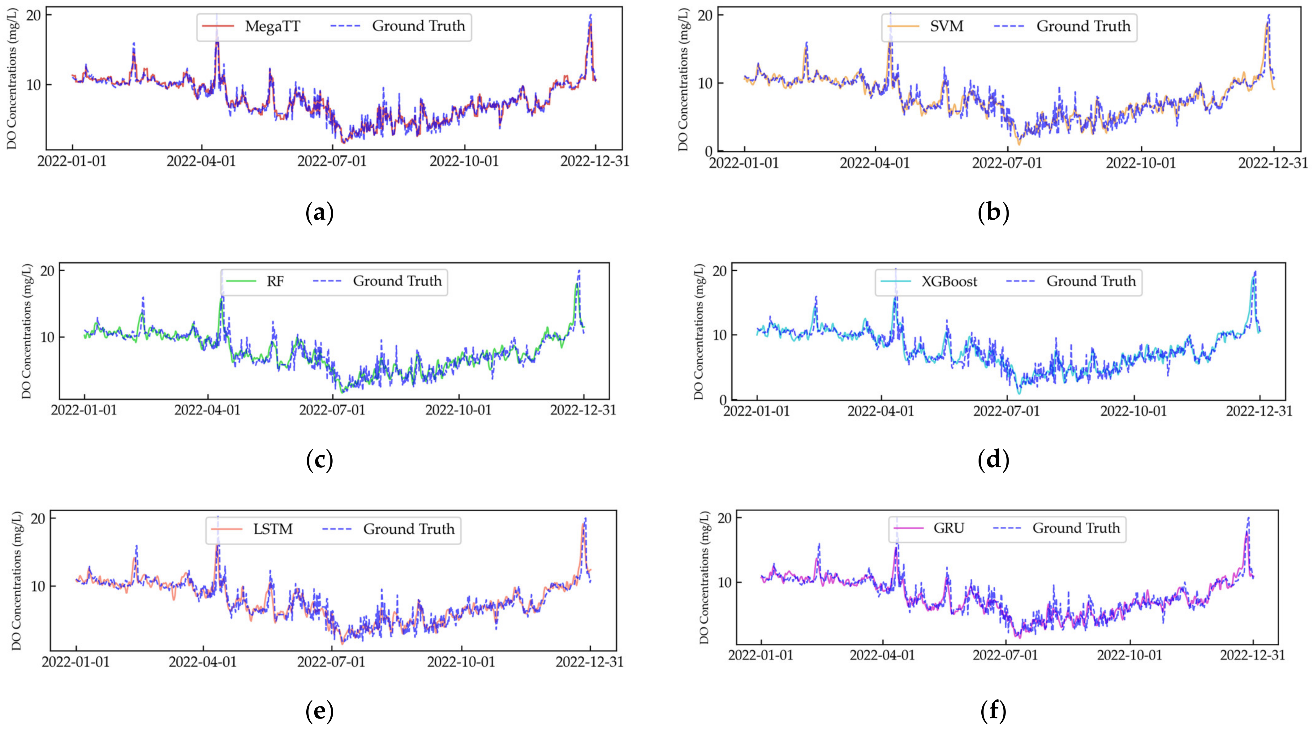
Figure 4 provides a visual time-series analysis, highlighting the comparative predictive accuracy of MegaTT and the benchmark models. It can be observed that the MegaTT model captures the variations in dissolved oxygen concentrations effectively, closely following the observed values. In comparison, although all models demonstrate competence in capturing the general trend, they fail to capture sudden changes or maintain consistent accuracy across the time span, a challenge efficiently tackled by our proposed MegaTT model.
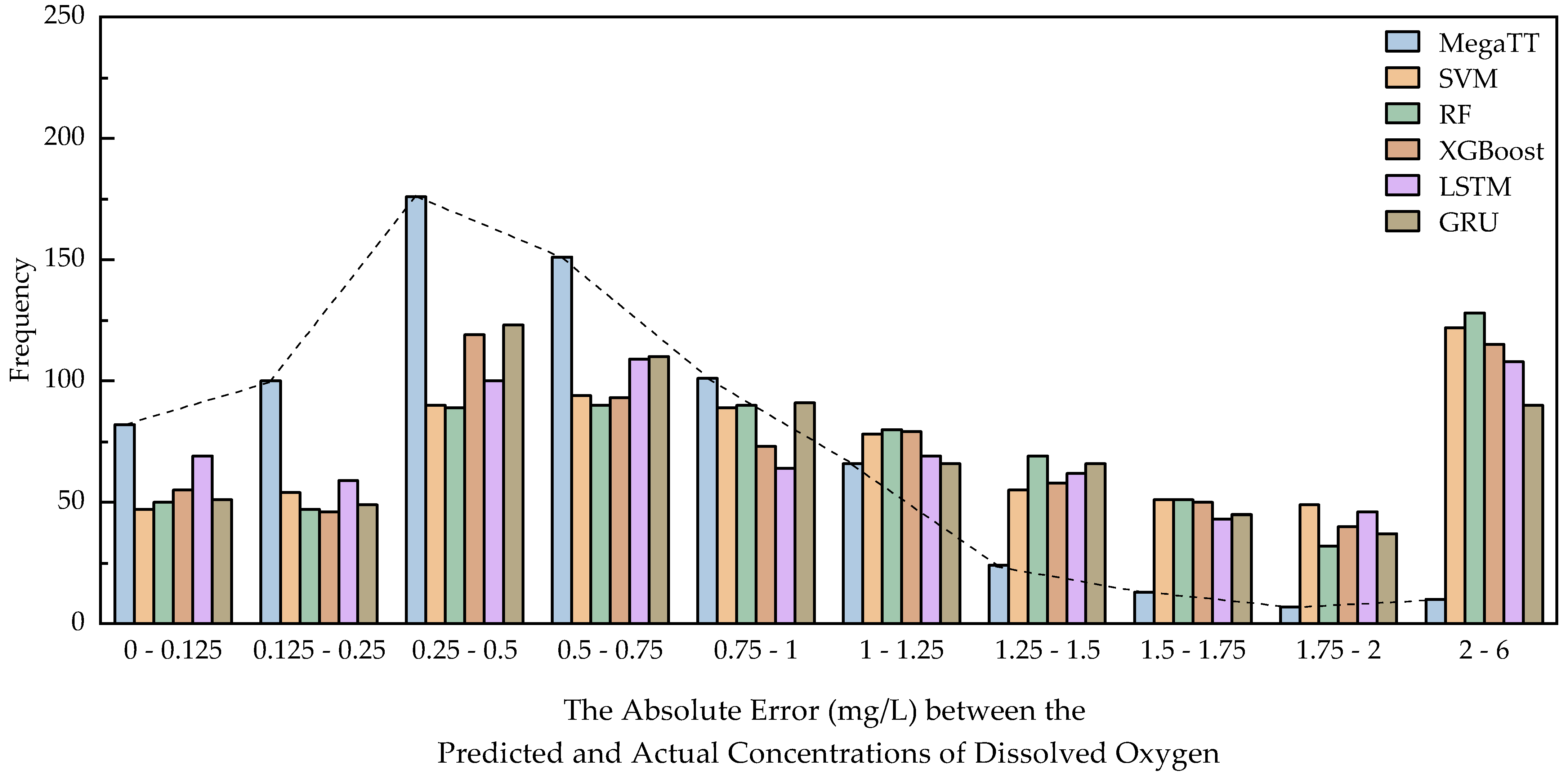
The comparative error distribution of all models is illustrated in
Figure 5. Here, we can observe that MegaTT’s prediction errors are mostly concentrated in lower error intervals, implying higher prediction accuracy. In contrast, other models demonstrate wider error distributions, indicating less stable predictive performances.
The comparative performance metrics are further tabulated in
Table 5. These results provide quantitative evidence to the superiority of MegaTT over the benchmark models. Specifically, MegaTT outperforms all other models with the lowest
RMSE and
MAE and the highest
R2 score. This implies that our MegaTT model achieves superior precision, lower tendency of large errors, and better consistency with the observed data.
In conclusion, through the rigorous comparisons in this section, it is unequivocally demonstrated that our proposed MegaTT model outperforms a variety of established models in the field. The superior performance is evident in both the time-series analysis and the error distribution, and it is further corroborated by the performance metrics. This suggests that our novel approach of employing the graph embeddings of meteorological stations, coupled with a temporal transformer for optimized predictions, provides a more robust and accurate tool for predicting dissolved oxygen concentrations in water bodies.
4.2. Impact of Meteorological Graph Connectivity Variation on Model Performance
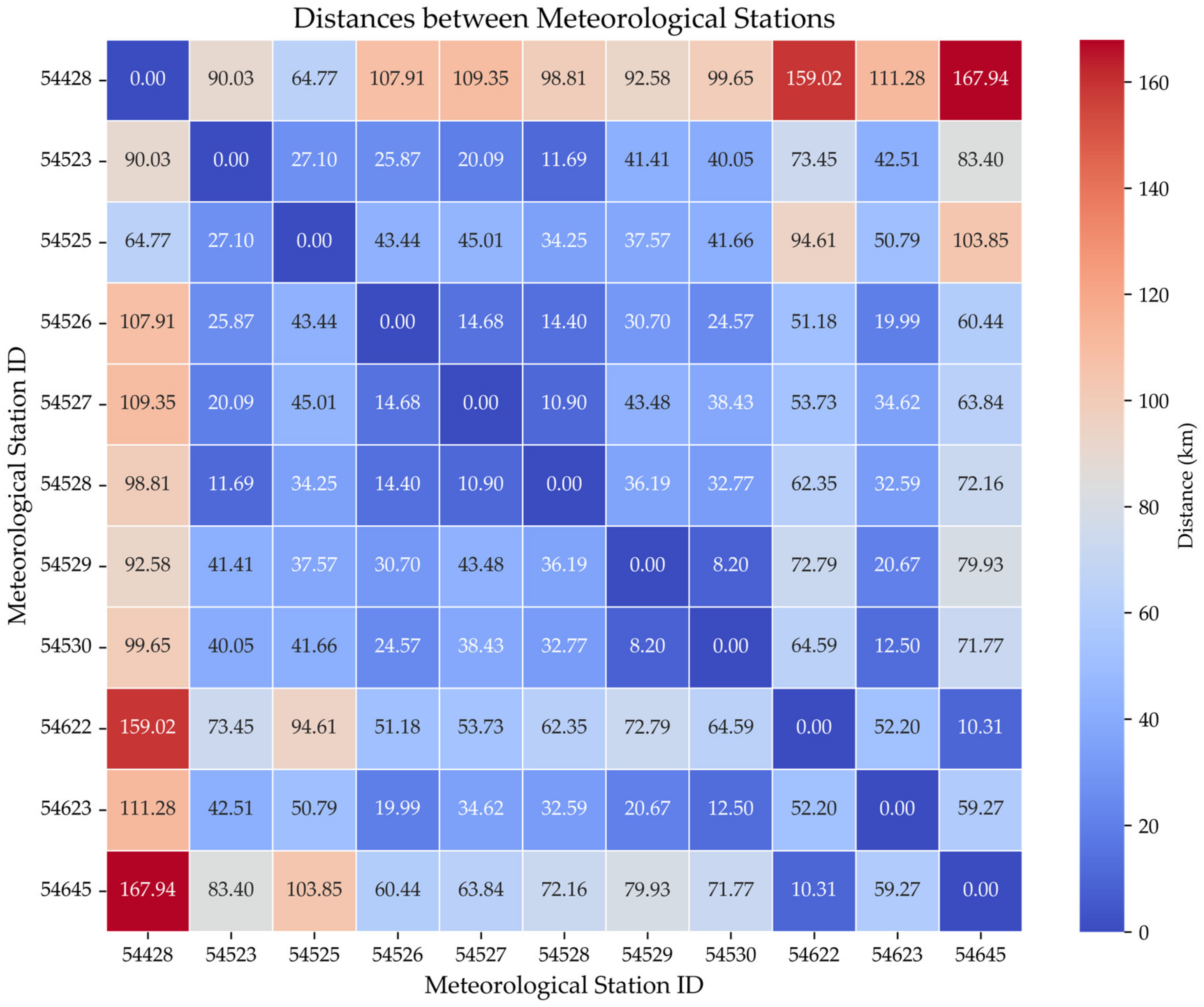
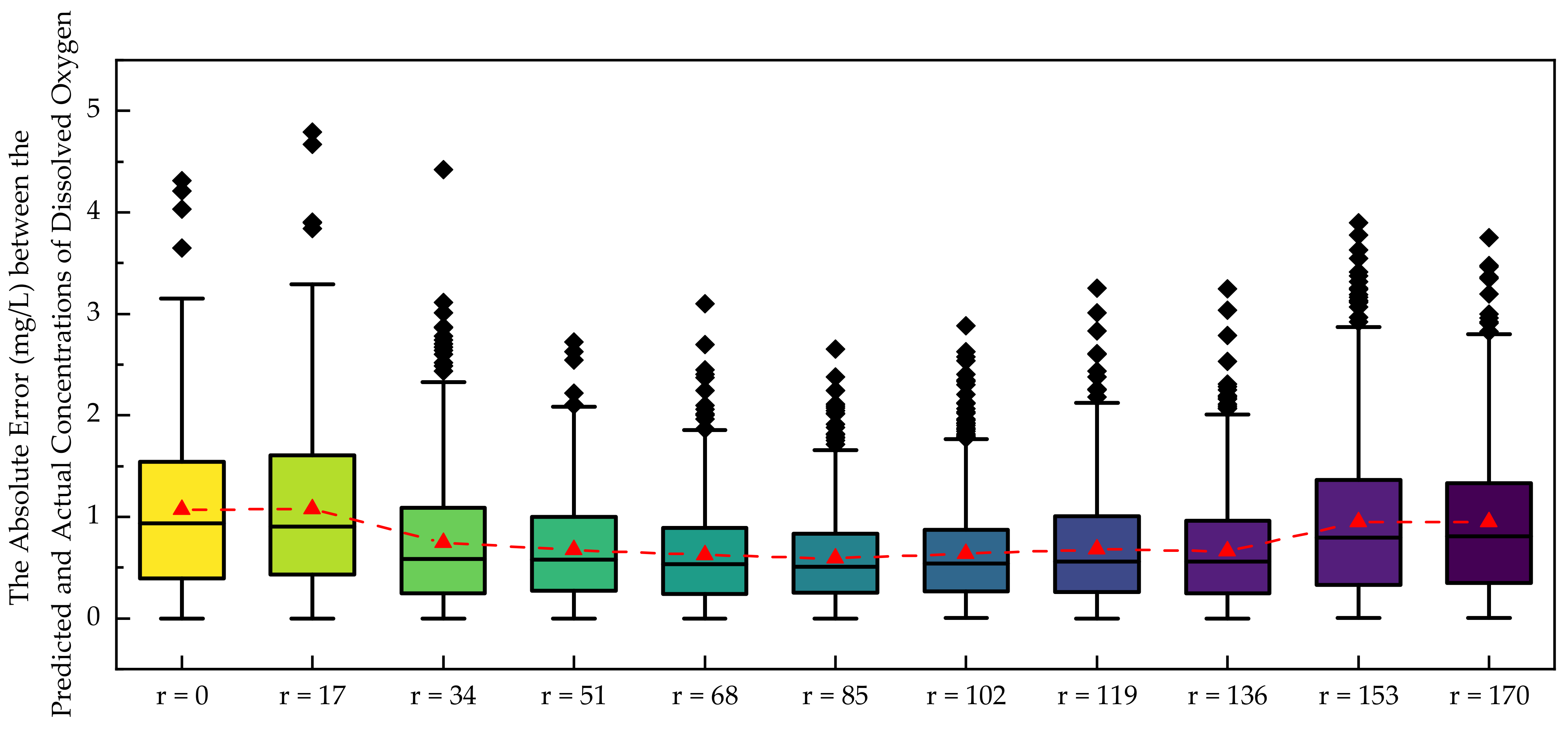
The role of meteorological graph connectivity in enhancing the prediction performance of the MegaTT model is explored in this section. In an effort to understand the effects of varying graph connectivity on the model’s performance, we incrementally adjusted the spatial threshold from zero (signifying no connections among vertices) up to 170 km (a distance surpassing the longest inter-station gap, thereby resulting in a fully connected graph).
Figure 6 serves as a heatmap of the spatial distances between the 11 meteorological stations and the resultant impact on model performance is illustrated in
Figure 7 and
Table 6.
Figure 7’s boxplot indicates the absolute prediction errors of the model corresponding to each spatial threshold. Each box’s median value is linked to visualize the trend of error variation with the changing threshold.
Notably, as the spatial threshold increased from 0 to 85 km, the model’s Root Mean Squared Error (RMSE) and Mean Absolute Error (MAE) exhibited a general downward trend, despite slight fluctuations. Concurrently, the coefficient of determination (R2) increased. This outcome suggests that, within this range, expanding the spatial threshold—thus broadening the information exchange between meteorological stations—enhances the model’s predictive accuracy for dissolved oxygen concentrations. It could be due to the fact that meteorological stations within this range likely capture similar atmospheric conditions, which contribute significantly to the dissolved oxygen concentration levels in the associated water bodies.
However, when the spatial threshold extended beyond 85 km, the RMSE and MAE began to climb while the R2 declined. This suggests that an excessively high threshold, leading to a fully connected graph, may introduce irrelevant associations. For example, meteorological stations that are geographically distant might not share similar atmospheric conditions, and forcibly connecting them could introduce noise into the model. Consequently, this unnecessary information exchange may distort the model’s learning, causing a decline in prediction performance.
Table 6 corroborates the observations from
Figure 7, revealing an optimal threshold of 85 km for constructing the meteorological graph, a key factor in the MegaTT model’s performance. This optimal threshold is vital for capturing the spatial-temporal structure of multi-site meteorological data. When the threshold was below 85 km, suburban meteorological stations 54622, 54645, and 54428 gradually disconnected from the main central city area meteorological graph, impacting the prediction accuracy. Conversely, when the threshold exceeded 85 km, the connections became overly dense, introducing noise and distorting the model’s learning. An 85 km threshold allowed for connections that were neither too dense nor too sparse, achieving the highest prediction accuracy for dissolved oxygen concentrations in the target area, located in the central city. This finding underscores the importance of a well-defined threshold for the meteorological graph, emphasizing the significance of balanced connections between remote suburban and central city meteorological stations. It not only enhances the prediction of dissolved oxygen concentrations but also provides essential guidance for future research on graph-structured environmental data analysis, laying a foundation for a more precise and robust modeling of environmental phenomena.
4.3. Ablation Study of Meteorological Module and Impact of Nearest Single-Station Approach
In this section, two principal experiments are designed to evaluate the effectiveness of the proposed MegaTT model in capturing meteorological factors that influence dissolved oxygen concentration predictions in water bodies.
The first experiment involves a comparison between the full MegaTT model and its reduced form, referred to as the Temporal Transformer (TT) model. By eliminating all meteorological station inputs and retaining only the Temporal Transformer Prediction Module, this comparison serves to highlight the contributions of the integrated meteorological modules in the MegaTT model.
The second experiment emphasizes a specific configuration, where only the meteorological factors from the nearest station are retained in the MegaTT model (NS-MegaTT).
Table 7 lists the distances between 11 meteorological stations and the target water quality monitoring site, highlighting the proximate relationships. Among them, station 54529 is identified as the closest to the target water quality monitoring site. By employing data exclusively from this nearest meteorological station, the analysis aims to assess the impact of nearest single-station information on the model’s capability in predicting dissolved oxygen concentrations accurately.
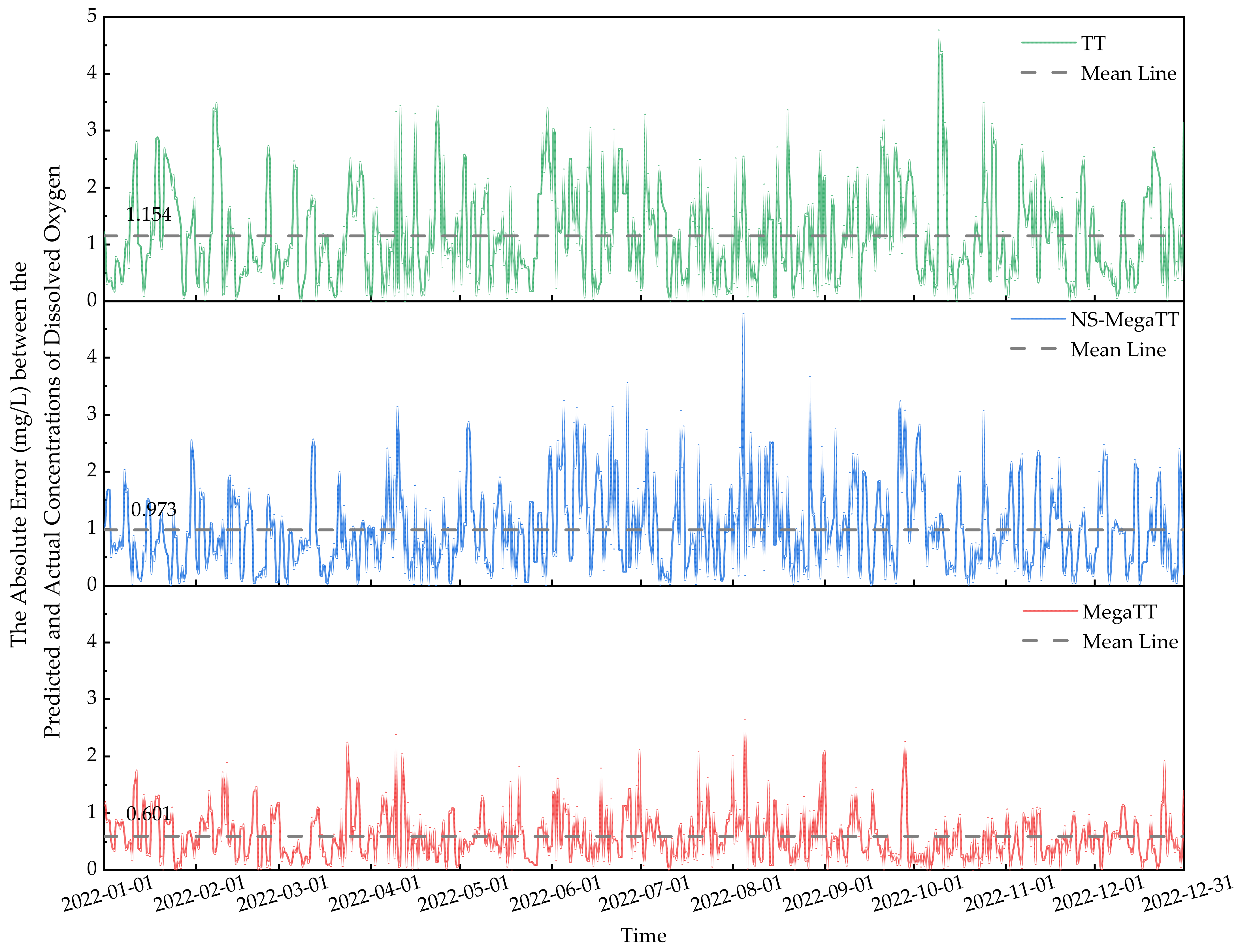
Figure 8 provides a visual representation of the absolute errors for each model. The grey dashed lines marking the
MAE in each subplot further elucidate the differences between the models.
The TT model, without meteorological inputs, displays higher errors (RMSE: 1.427, MAE: 1.154) and a relatively lower determination coefficient (R2: 0.798). NS-MegaTT, which incorporates data only from the nearest meteorological station, improves performance slightly (RMSE: 1.236, MAE: 0.973, R2: 0.848). The full MegaTT model shows substantial improvements with the lowest errors (RMSE: 0.754, MAE: 0.601) and the highest determination coefficient (R2: 0.936). The comparison emphasizes the contribution of multi-station meteorological data in predicting dissolved oxygen concentrations. The MegaTT model’s superiority is apparent, with significantly better performance in terms of error minimization and R2 value.
The results of the ablation study offer profound insights into the importance of meteorological data integration. The MegaTT model’s significant enhancement in prediction accuracy underscores the effectiveness of the dynamic meteorological graph construction.
5. Conclusions
This study aimed to enhance the prediction of dissolved oxygen concentrations in water bodies through a novel approach, the Meteorological Graph and Temporal Transformer (MegaTT) model. This model effectively exploited the spatial-temporal structure of multi-site meteorological data, providing a comprehensive understanding of the water bodies’ characteristics and their impacts on dissolved oxygen concentration predictions.
Our MegaTT model outperformed traditional machine learning models, including Support Vector Machine (SVM), Random Forests (RFs), Extreme Gradient Boosting (XGBoost), Long Short-Term Memory (LSTM), and Gated Recurrent Unit (GRU), demonstrating its superiority in handling complex geospatial and temporal patterns.
Furthermore, the study determined an optimal distance threshold of 85 km for constructing the meteorological graph, achieving the highest prediction accuracy for dissolved oxygen concentrations in the target area. This threshold maintained a balanced connection between remote suburban and central city meteorological stations. This finding emphasizes the importance of carefully defining connections within the graph and provides essential guidance for future research on graph-structured environmental data analysis.
An ablation study further underscored the essential role of the meteorological module, with the MegaTT model significantly outperforming its reduced versions, namely the Temporal Transformer (TT) model and the Nearest Single-Station MegaTT (NS-MegaTT). This in-depth analysis provided a robust justification for integrating multi-station meteorological data, leading to improved dissolved oxygen prediction accuracy.
The MegaTT model presented in this paper opens up a new perspective on dissolved oxygen concentration predictions. It not only shows promising results but also paves the way for the potential incorporation of other environmental factors, advancing the development of holistic and effective water quality management strategies. Future research directions could involve exploring other types of environmental data and applying the MegaTT model to different water quality parameters, which would be of great significance for environmental management and policymaking.
