Article

Groundwater Level Trend Analysis and Prediction in the Upper Crocodile Sub-Basin, South Africa

by
Tsholofelo Mmankwane Tladi
1,*,
Julius Musyoka Ndambuki
1,
Thomas Otieno Olwal
2 and
Sophia Sudi Rwanga
3
1
Department of Civil Engineering, Tshwane University of Technology, Pretoria 0183, South Africa
2
Department of Electrical Engineering, Tshwane University of Technology, Pretoria 0183, South Africa
3
Department of Civil Engineering Science, University of Johannesburg, Johannesburg 2006, South Africa
*
Author to whom correspondence should be addressed.
Water 2023, 15(17), 3025; https://doi.org/10.3390/w15173025
Submission received: 17 July 2023 / Revised: 16 August 2023 / Accepted: 16 August 2023 / Published: 22 August 2023
(This article belongs to the Section Hydrology)

Abstract

:
Disasters related to climate change regarding water resources are on the rise in terms of scale and severity. Therefore, predicting groundwater levels (GWLs) is a crucial means to aid adaptive capacity towards disasters related to climate change in water resources. In this study, a Gradient Boosting (GB) regression modelling approach for GWL prediction as a function of rainfall and antecedent GWL is used. A correlation analysis carried out from 2011 to 2020 demonstrated that monthly GWLs can be predicted by antecedent GWLs and rainfall. The study also sought to understand the long-term effects of climate events on groundwater levels over the study area through a Mann–Kendall (MK) trend analysis. A total of 50% of the groundwater stations revealed declining trends, while 25% had no trends and the other 25% showed an increasing trend. Again, the correlation analysis results were used in justifying the trends. The GB predictive model performed satisfactorily for all groundwater stations, with the MSE values ranging from 0.03 to 0.304 and the MAE varying from 0.12 to 0.496 in the validation period. The R2 ranged from 0.795 to 0.902 for the overall period. Therefore, based on projected rainfall and antecedent groundwater levels, future GWLs can be predicted using the GB model derived in this study.

1. Introduction

Climate change has led to a recurrence of hydrological extremes such as droughts and floods and future projections reveal an increase of such events [1,2]. Mishra & Singh [3] reported a number of droughts in Africa, Europe, Asia, Australia and North America dating as far back as 1890. Wanders et al. [4] projected an increase in drought duration and severity over 27% of the world; this includes most parts of South America, Southern Africa and the Mediterranean. Most parts of Southern Asia have been experiencing accelerated droughts due to rising temperatures in the past few decades [5,6]. In Uganda, 2465 human lives were lost due to droughts, and this was globally the highest mortality due to droughts in 2022 [7]. Climate change has also led to a number of floods at a global scale, which resulted in 7954 human lives lost in 2022 [7]. This number exceeds the global average from 2002 to 2021. Countries with the highest mortality due to floods in 2022 include India at 2035, Pakistan at 1739, Nigeria at 608 and South Africa at 544 lives [7].
The impacts of these hydrological extremes in an arid to a semi-arid country like South Africa are significant. For example, the droughts experienced in most parts of the country in the hydrological year 2015 to 2016 led to negative socio-economic impacts [8]. The agricultural industry contracted by 6.5%, while the electricity, gas and water industry contracted by 2.8% in the first quarter of 2016 [8]. Various parts of the country experienced water restrictions due to the droughts. These droughts in the Western Karoo region of the Eastern Cape province occurred until early 2020 [9]. The multi-year drought in the Eastern Cape resulted into low groundwater levels and subsequently dried up some boreholes [10]. On the other hand, the neighbouring province, Kwa Zulu Natal (KZN), has been experiencing frequent floods, like in April 2019 [11,12]. Recently, in April 2022, KZN experienced one of the major floods in the country, resulting in over 400 lives lost over the disastrous floods [13]. What is evident in literature is that disasters related to climate change are on a steep rise, but the adaptive capacity towards these extreme events seems to be lacking [14,15,16]. This gap, coupled with freshwater scarcity, thus exacerbates the importance of understanding the interplay between climate and water resources, and such knowledge is essential for the sustenance of water resources.
The growing number of extreme climate events and population growth have further strained surface water resources, making it an unreliable source. Groundwater thus plays a vital role in an arid to semi-arid region like South Africa. A study by the Department of Water and Sanitation [17] revealed that an additional 7500 million m3 per annum of groundwater storage was available for use by small towns, mines, villages and individuals. Moreover, this groundwater potential could be increased by recharging aquifers during wet periods and preserving groundwater supplies for use during dry/drought periods [18]. Pietersen et al. [18] further showed that over 80% of rural communities in the North West and the Kwa-Zulu Natal provinces of South Africa receive their water from groundwater sources, and the same applies to over 50% of communities in the Eastern Cape Province. In terms of urban areas, the City of Tshwane combines water from boreholes with surface water in its bulk distribution system. Some towns such as De Aar rely solely on groundwater sources for their water supply.
Groundwater availability is affected by a wide range of factors which include land use land cover (LULC), baseflow index, which refers to the proportion of baseflow to the total streamflow [19], soil type, catchment area, catchment slope, precipitation, evapotranspiration and catchment geology [19,20]. Precipitation is by far the climatic parameter that most closely relates to groundwater availability and water resources in general, serving as a major input into the hydrological cycle. In South Africa, the most available form of precipitation is rainfall. Rainfall, according to a study conducted by Mohan et al. [21] was found to be one of the major factors that contributes to groundwater recharge. A similar study in the United States of America also found that 80% of recharge variation is explained by Mean Annual Precipitation [22]. Similarly, findings by Sun & Cornish [23] revealed that variations in recharge can primarily be explained by the climatic factor compared to land-use changes. The studies outlined above illustrate the importance of rainfall events in groundwater recharge. Recently, there has been a growth in representing groundwater systems through models, and models also aid in understanding the interplay between processes involved in a system.
There is, however, a lack of data on the actual use of groundwater resources, and the state of aquifers is unknown in many parts of the world. Modelers are faced with dispersed data or data scarcity, especially in arid to semi-arid areas. Data such as aquifer geometry or hydraulic parameters are often unknown [24,25]. Monitoring networks and consistent in situ groundwater measurements are unavailable in some places [26]. There are inaccuracies in recharge and pumping estimates [27].
Various groundwater quantity models have been used in the past to enhance the management of groundwater resources. The models include physically based numerical models such as MODFLOW [28,29], data-driven models employing artificial intelligence [26,30], and a hybrid of the two [31,32,33]. In the past, physically based numerical models were extensively employed in modelling and predicting groundwater levels [34,35]. The physically based numerical models, however, are often time-consuming, require extensive amounts of input data that are often not available and require some level of expertise in measuring the parameters used in the models [36]. The growing availability of big data, through remote sensing and the Internet of Things (IoT) have made data-driven modelling such as machine learning (ML) a favourable modelling tool. Machine learning is a field of artificial intelligence that employs algorithms to learn complex patterns from data and is able to predict unobserved data [37,38]. According to Osman et al. [39], ML models are estimated to be adequately efficient in modelling groundwater levels. Artificial Neural Networks (ANNs) and Support Vector Machines (SVM) rank amongst the widely used ML models in groundwater level modelling [34,36]. Recently, a growth in the use of ensemble machine learning techniques has been observed and one of the advantages that the ensemble techniques offer is lower computational cost [40]. One of the commonly used ML ensemble techniques is the Gradient Boosting (GB) algorithm. The GB algorithm was successfully used in Iran for predicting monthly GWL [36]. In Slovenia, GB outperformed linear regression, random forest and decision tree algorithms for predicting GWLs. Again, in a Moroccan study, where ten ML models were compared in predicting groundwater withdrawals, GB outperformed all the algorithms [41]. In a South African study, GB also outperformed five ML algorithms, among which ANNs and Support Vector Regression (SVR), the dominantly used ML algorithms, were included [42].
The common limitations among ML algorithms are that they lack interpretability and they are often subjected to overfitting problems [40,43]. Some of the ML algorithms have limitations to non-linear and non-stationery processes [44] and would often require modifications of the ML algorithm [40,44]. SVMs, for example, are generally sensitive to input parameter selection [45], while GB, on the other hand is known to handle a wide range of input parameters, is resistant to non-stationery processes, and is more robust to outliers [46,47]. Despite the accuracy and computational efficiency of GB, literature on the use of ensemble ML techniques such as GB in predicting GWL is still lacking [36,39].
The selection of optimal input variables in ML modelling is an essential step. Some methods that can be used in the selection of input variables include principal component analysis, stepwise approach [48], mutual information [38,42] and correlation analysis. In time series studies, optimal lags also need to be selected. Autocorrelations, partial autocorrelations and cross-correlations are among the most efficient statistical methods for the selection of lag times in artificial intelligence (AI) modelling techniques [42,49]. Few studies, for example, Derbela & Nouiri [50], used correlation analysis in predicting groundwater levels through ANN, and Wei et al. [40] employed correlation analysis in selecting input variables for groundwater level prediction through Support Vector Machines (SVM) and Random Forest (RF) [51]. Literature on the application of correlation analysis in the selection of lags for AI models is, however, still lacking [49].
Considering the growing rate of disasters related to climate change, freshwater scarcity and the gap that exists in adaptive capacity to climate change related disasters, there is a need for a proactive approach in managing groundwater resources. An envisioned groundwater management system should comprise a monitoring component that analysis historical data, monitors real time or near real time conditions [52] and predicts future groundwater conditions [53]. This study focuses on the historical data analysis and the prediction component of an envisioned groundwater management system. The main goal of this study is to predict GWLs, and it was broken down into the following objectives: (1) To evaluate the strength of the relationships and determine lag times between input variables and the response variable using autocorrelations, cross-correlations and multiple correlations. (2) To gain an understanding of the effects of climate events on groundwater levels over a decade through a trend analysis. (3) To predict GWLs in quaternary A21D of the Upper Crocodile sub-basin through a ML approach. To the best of our knowledge, no works in the literature were found that used correlation analysis in the selection of input variables for GWL prediction through GB, especially in the South African context.

2. Materials and Methods

2.1. Study Area Description

The study area is the Upper Crocodile (West) located in the North-West and Gauteng province of South Africa. Its geographic location is between the coordinates −25.678 latitude; 27.341 longitude and −25.678 latitude; 28.472 longitude. The towns covered in the Upper Crocodile (West) area are Krugersdorp, Magaliesburg, Centurion, Midrand and Kempton Park. This basin is the second-most-populated basin in the country [54].
The Upper Crocodile is a semi-arid region. It is characterised by warm summers with average daily minimum temperatures of 10 °C to maximum temperatures of 30 °C and cold winters with minimum temperatures of 1 °C to maximum temperatures of 15 °C [54]. The rainy season is in summer, which commences in October and ends in March the following year. Rainfall usually peaks in December and January. The mean annual rainfall ranges between 600 mm and 800 mm per annum [55]. The mean annual evaporation exceeds the mean annual rainfall, with the mean annual evaporation at an average of approximately 1600 mm per annum [54].
Hydrologically, the Upper Crocodile (West) falls under the Limpopo water management area, primary drainage region A. The primary drainage regions are further broken down into secondary, tertiary and subsequently quaternary drainage regions. To be more exact, the Upper Crocodile (West) is in the secondary drainage region A2 and tertiary drainage A21. For this study, the quaternary drainage regions lying upstream of the Hartbeespoort dam were considered, which make up approximately 4100 km2 (quaternary drainage A21A to A21H). The main rivers in the Upper Crocodile are the Crocodile, Magalies, Jukskei and Hennops. The main dams are the Hartbeespoort dam in quaternary A21H and the Rietvleidam in A21A. Figure 1 below displays the study area.
The main source of water supply in the study area is the Vaal dam, which is transferred through the Rand Water bulk distribution system from the Upper Vaal Water Management Area. The other important source of water supply in the study area is groundwater from dolomitic aquifers, which are mainly found in the quaternaries: A21A (North East of Johannesburg), quaternary A21B (near Centurion) and quaternary A21D (near Krugersdorp). Dolomite-based aquifers (karst aquifers) are among the most prolific water-bearing formations due to their soluble nature [56]. Groundwater from these karst aquifers is used in the City of Tshwane, North East of Johannesburg and Krugersdorp area for agricultural, domestic and industrial use [54]. Projections reveal more potential for the usage of this groundwater resource [57], which may be beneficial for this rapidly developing area.
The Upper Crocodile is characterised by karst aquifers, which are generally deep and high-yielding, as well as fractured aquifers which are shallow and have lower yield [56]. The specific yield of the fractured aquifers in the study area ranges between 0.01 L/s and 0.98 L/s, while the karst aquifers’ yield is in the range of 15 L/s to 124 L/s. Approximately 10% of the City of Tshwane’s water supply is from these Karst aquifers. Recharging the karst aquifers in Gauteng ranges between 7% to 15% of the mean annual precipitation (MAP) [57], and this could be attributed to the mean annual evaporation, which far exceeds the MAP. Borehole depths in the karst aquifers reach 250 m depth and water table levels can go below 10 m to 50 m [54]. The economic activities taking place in the Upper Crocodile are mainly industrial, mining and residential, which contribute a significant amount of the country’s Gross Domestic Product (GDP) [54]. This study area was chosen because of groundwater data availability and the economic importance of this area in South Africa. Due to the availability of consistent data, the existence of shallow boreholes in the area and the high spatial–temporal variability of the parameters under study, this study focused on quaternary A21D of the Upper Crocodile. The total area of A21D is 371.54 km2.

2.2. Data Sources and Acquisition

Daily rainfall data were obtained from the South African Weather Service (SAWS). The station that was selected for data analysis was 05127467, shown in Figure 1. The choice of this station was informed by historical data availability and the proximity of the rainfall station to shallow groundwater monitoring stations. The station is located at latitude −25.9436 and longitude 27.9188, as shown in Figure 1.
Groundwater data were obtained from the Department of Water and Sanitation (DWS) through the National Ground Water Archive, available online. The stations that were selected for analysis in this study are shown in Table 1. Most of these stations are shallow and were selected based on data availability. Also, the stations, unlike most stations, had daily groundwater levels in some instances. All the stations listed in Table 1 are still active.
Raw hydrometeorological data very rarely come complete and ready to use, especially in situ data, as a result cleaning and processing is required. One of the major challenges incurred with raw time series data is the inconsistent frequency of data collection, handling blanks and the data size is often big to detect the errors using the human eye. This particular groundwater dataset came with inconsistent frequencies; the frequencies were first fixed to a monthly frequency using the resample function in Pandas. Pandas is a data analysis tool built in the Python Programming language. After fixing the time frequency using the function ‘pd.to_datetime’, the missing groundwater levels were filled in using the function ‘resample(‘M’).mean()’, which replaces the blanks with the mean between the two available measurements.
The existence of outliers in in situ data is also common and needs to be scrutinized in the early stages of data cleaning and processing. Outliers are defined as the minority of the observations in the dataset that have different patterns from the majority of the observations in a dataset [58]. The analysis of outliers in both the rainfall and the groundwater data was carried out using the traditional boxplot outlier detection method [59,60].
Two extreme values in the upper range were identified from the rainfall data and fell under the rainy seasons. These extreme values were not removed from the dataset as they were representative of the high rainfalls that occurred in the study area in early 2017 and 2018. All groundwater stations had extreme values except for groundwater station A2N0794. The percentage of the extreme values for the groundwater stations ranged from 2% to 8% of the dataset. These extreme values were also not removed from the data set, as the extremes agree with what is expected during the period in which they were encountered in the study area, for example, extremely deep groundwater levels towards the end of the non-rainy seasons or shallow groundwater levels during rainy seasons or just after the rainy season.

2.3. Methods

2.3.1. Correlation Analysis

(a)
Cross correlation analysis
A cross-correlation function measures the strength of a linear relationship between two time series data depending on a time lag between them [61]. It assesses the similarity between a time series and a lagged version of another time series as a function of the lag [62]. Theoretically, the cross-correlation functions are explained in Equation (1) to Equation (2) [61], where x represents the input time series while y represents the output time series from a hydrological system. Equation (1) defines the covariance function between x and y , both with length n .
c x y k = 1 n t = 1 n k x t μ x y t + k μ y ; k = 0 , ± 1 , ± , , m
where μ x is the mean of x and μ y is the mean of y . m is the time interval in which the analysis is carried out or rather the total number of correlation coefficients obtained from the analysis, and k is the number of time lags. Equation (2) defines the cross-correlation function between time series x and y .
r x y k = c x y k σ x σ y ; k 0 c y x k σ x σ y ; k < 0
where σ x is the standard deviation of x and σ y is the standard deviation of y .
The application of cross-correlations play a vital role in hydrology, and this is evident in, Rahmani & Fattahi [62], Seo et al. [63] and Valois et al. [64]. What is common in the three studies is that the studies cross-correlated climatic parameters with the availability of water resources, with Valois et al. [64] focusing on precipitation and groundwater recharge, which is closely related to this study, while Seo et al. [63] demonstrated the importance of pre-processing climate data through using cross-correlations. In the study it was deduced that precipitation and temperature cross-correlations aid in improving hydrologic simulations. One of the vital features of cross-correlation analysis is its ability to express the interdependence of parameters, a feature that is helpful in selecting input parameters for models that are data-driven. In this study, rainfall was cross-correlated with groundwater levels for the study period 2011 to 2020, and the data were analysed at a monthly time step k . Cross-correlations between rainfall from rainfall station 0512746 7 and the eight groundwater stations selected for this study were computed, and the highest possible lags for this analysis was 117 lags k .
(b)
Autocorrelation Analysis
Groundwater level fluctuations are greatly influenced by historical groundwater levels [40], and thus knowledge on how the previous month’s groundwater levels affect the succeeding month’s groundwater levels is essential. Autocorrelation analyses were thus conducted in this study to determine the interdependence of succeeding groundwater levels and to determine the optimal lag between succeeding records. An autocorrelation function refers to the measure of strength of the linear relationship among succeeding values in a time series depending on the lag time between the values [61]. The function is represented in Equation (3):
r x x k = c x x k σ x 2   ; k 0
In this study, an autocorrelation analysis was performed on historical groundwater levels for the study period 2011 to 2020.
(c)
Multiple correlation analysis
Lastly, multiple cross-correlation analysis was carried out, which reveals the strength of the relationship between more than one independent variable with the one dependent variable. The independent variables in this study were rainfall, representing the climate aspect, and antecedent GWLs, representing the hydrogeological aspect of the analysis.

2.3.2. Trend Analysis

The Mann–Kendall test was applied for studying trends for data obtained from eight groundwater stations. Figure 1 shows the location of the groundwater stations in relation to one another and the rainfall station. The Mann–Kendall test is a non-parametric test used to identify trends in time series data [65]. The test has successfully been used in analysing hydro-meteorological datasets concerning climate, environmental parameters, streamflow and groundwater levels in the past [66,67,68]. One of the advantages of this test is that it does not require data to be normally distributed [68], and hydrometeorological data are usually not normally distributed. The Mann–Kendall test is founded on the correlations between sequences and ranks. In this test, a test statistic S is obtained by computing the difference between subsequent data values. Equations (4)–(8) describe the test and xi and xj in the equations represent the values of a sequence where j is greater than i and n represents the length of the time series. The Mann–Kendall statistic (S) is given as [65]:
S = i = 1 n 1 j = i + 1 n s g n x j x i i = 1 n 1 j = i + 1 n s g n θ
where s g n θ satisfies any of the following conditions:
s g n θ = 1   i f   θ > 0 0   i f   θ = 0 1   i f   θ < 0
When n ≥ 8, the statistic S is approximately normally distributed with the mean and variance, as follows:
E S = 0
V S = n n 1 2 n + 5 i = 1 m t i   i i 1 2 i + 5 18
where m   is the number of groups of tied ranks and t i   is the number of ties of extent i. The standardized Z M K is computed as follows:
Z M K = S 1 V a r S   S > 0         0           S = 0 S + 1 V a r S   S < 0
ZMK measures the significance of the test. In this study, the null hypothesis (H0) assumed that there is no trend, while the alternative hypothesis (H1) assumed that there is a trend. The null H0 was rejected if Z M K > Z 1 α at a significance interval of α = 0.05. The Mann–Kendall analysis was conducted using Python.

2.3.3. Gradient Boosting Regression

Gradient boosting (GB) regression is a machine learning technique that uses ensemble trees by stacking them additively to provide final predictions [36]. It sequentially adds predictors to an ensemble, with each predictor correcting its predecessor [69]. A GB model consists of the predictor and response variables, a base learner, a differential loss function and a number of iteration trees. In each iteration, a negative gradient is calculated, the base learner function is fitted to the negative gradient, and then the base learner function is trained and the best gradient is found.
The algorithm GradientBoostingRegressor from the Scikit-learn library of ML in Python was employed in this study. The input variables for the predictive model were antecedent groundwater levels and rainfall. Rainfall (R) and antecedent groundwater level were the most used input variables for predicting GWLs using ML models [34]. In this study, the choice of these input variables was informed by the results obtained from a correlation analysis (autocorrelation, cross-correlation and multiple correlation coefficients). Lag times for the input variables were generated using cross-correlations for rainfall and autocorrelations for antecedent groundwater levels. Training data for the model were from January 2011 to April 2018, which was around 75% of the dataset, and validation data were from May 2018 to September 2020, which was around 25% of the dataset. Generally, a minimum of 70% to 90% of dataset is used for calibration [50]. Hyperparameter tuning was carried out using GridSearchCV for the selection of optimal parameters. GridSearchCV is a function found in the Scikit-learn library for ML using Python. The maximum depth of decision trees was selected as 2, the learning rate was selected within the set {0.15,0.01,1,10} and the number of trees were chosen between the set {10,50,250,900}.

2.3.4. Support Vector Regression

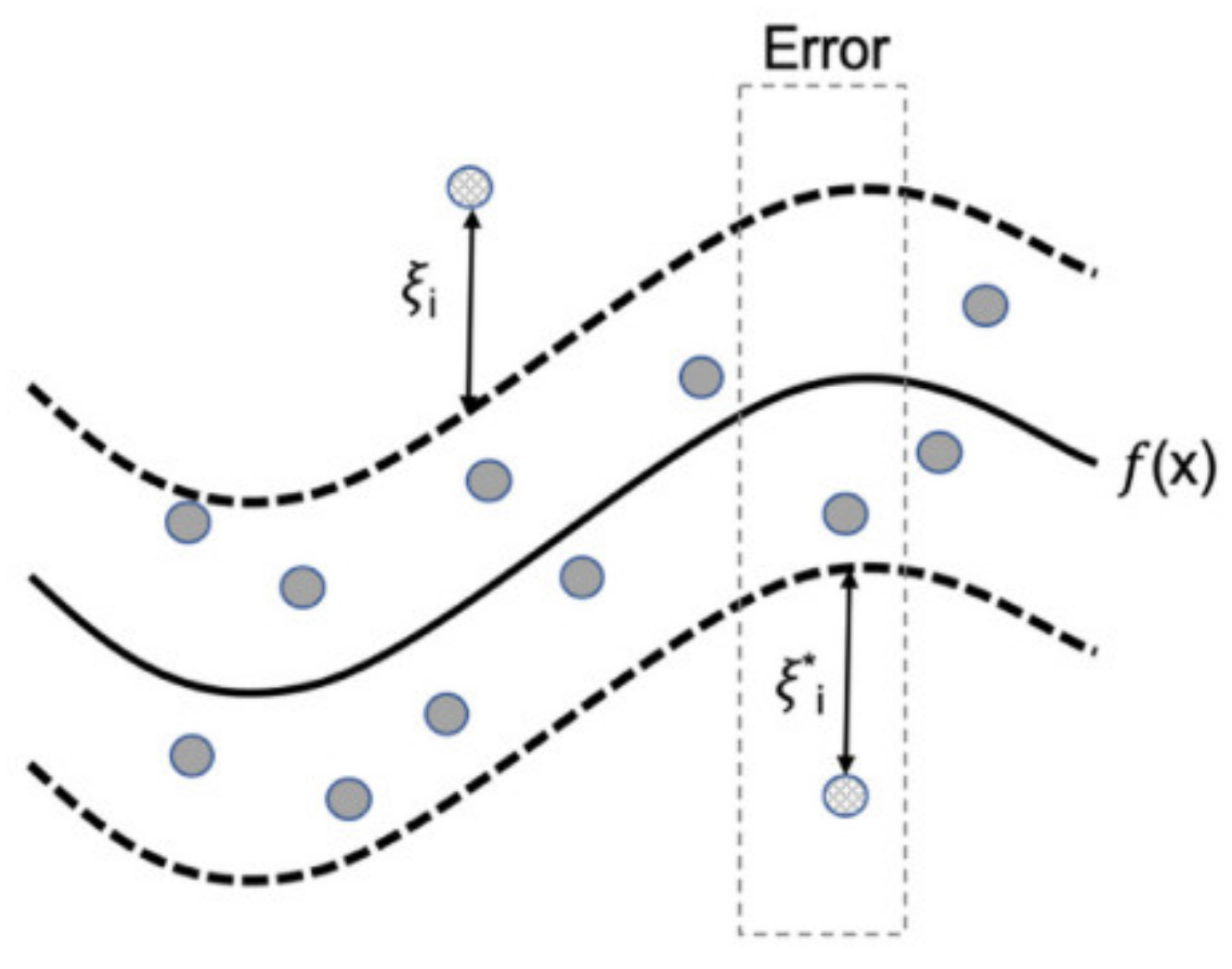
Support Vector Machine (SVM) is a machine learning algorithm based on the structural risk minimization (SRM) principle [70]. SVMs are used in classification and regression problems. When an SVM is applied in a regression problem, like in this study, wherein continuous data is predicted, groundwater levels, the regression component of SVM, named Support Vector Regression (SVR), is applicable. Figure 2 depicts the principle behind SVRs, and ε in Figure 2 is a precision parameter which represents the radius of the tube located around the regression function f(x). In an SVR, a kernel function maps inputs into a higher dimensional space and the SVR then considers a training data set and attempts to estimate a function with less deviation than ε from the observed target for all input data values [30,71].
In this study, the SVR algorithm was employed in predicting GWLs using antecedent GWL and rainfall as input variables. SVR has been extensively used in the literature to model GWLs when compared to GB, and thus the algorithm was introduced in this study to check the performance of GB. The training data for the SVR model were around 75% of the dataset, while the validation model was around 25% of the dataset. The model hyperparameter tuning used GridSearchCV for determining the optimal parameters to use for the model. The main parameter used in tuning the model was the epsilon ε in the range 0 to 1.5.

2.3.5. Performance Evaluation of Predictive Models

The performance of the predictive model was evaluated using the coefficient of determination (R2), the Mean Squared Error (MSE) and the Mean Absolute Error (MAE). The expressions for R2 and MSE are given in (9) to (11), respectively.
R 2 = i = 1 n O i S i S i S ¯ i = 1 n O i O ¯ 2 0.5 i = 1 n S i S ¯ 2 0.5 2
M S E = 1 n i = 1 n O i S i 2
M A E = 1 n O i S i
where Oi = observed data, Si = predicted data, O ¯ = mean of observed data, S ¯ = mean of predicted data and n = number of observations.
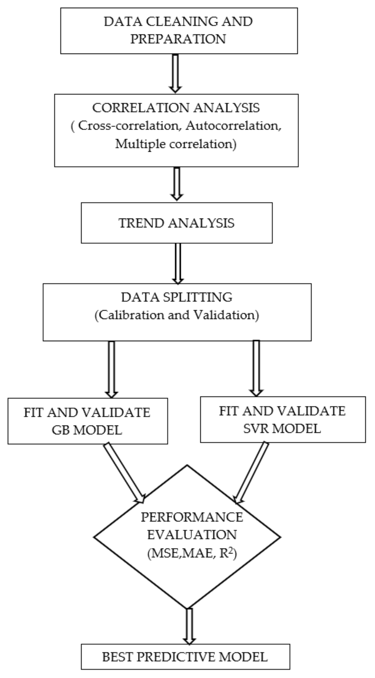
R2 describes the proportion of the variance in observed data explained by the model; its values range between 0 and 1, with values close to 1 indicating a variance with less error and values close to 0 indicating a high error variance. MSE measures the average of the squares of the errors. The MSE is always positive, and it is 0 for predictions that are completely accurate. It captures the bias (i.e., the difference of estimated values from the actual values) and variance (i.e., how far are the estimates spread out). An MAE value of 0 represents a completely accurate prediction model. Figure 3 depicts the workflow of arriving at the predictive model.
The data were firstly cleaned, and then a correlation analysis was carried out using cross-correlations, autocorrelations and multiple correlations. The correlation coefficients and the lags obtained were used in selecting the optimal input variables for the predictive model. The correlation coefficients were also used in interpreting the trends obtained in the study. After determining the optimal input variables, the data were split into the calibration and validation dataset. The SVR and the GB models were then trained and validated. A performance evaluation of the two models was carried out and informed the choice of the final predictive model for the study.

3. Results and Discussions

3.1. Correlation Analysis

Correlation analyses were carried out on a total of eight stations for the selection of input variables in the predictive model and to aid trend analysis. Four stations were ultimately selected for reporting and are presented in Table 2. The maximum cross correlation coefficients (CCmax), which represent the correlation between rainfall (R) and groundwater levels (GWL), were the lowest at a range of 0.145 to 0.288. The low CCmax can be associated with the underlying hydrogeological parameters, as rainfall is not the only variable that affects groundwater table fluctuations, although it is the main source of recharge. Also, the weak CCmax can be attributed to the spatial-temporal resolution at which the GWLs are measured, which is at a monthly time step in most of the stations. The autocorrelation coefficients (ACF) representing the response of predicted GWL to antecedent GWL were reasonably high, ranging between 0.851 and 0.940.
Lastly, the multiple correlations coefficients represent the combined effect of R and antecedent GWL to the dependent variable. They are the highest among the correlation coefficients in Table 2, at a range of 0.858 to 0.955. This thus implies that the combined independent variables, which are R at a 2-month lag and antecedent GWL at a 1-month lag, are valid for use as predictors for the predictive model.

3.2. Trend Analysis

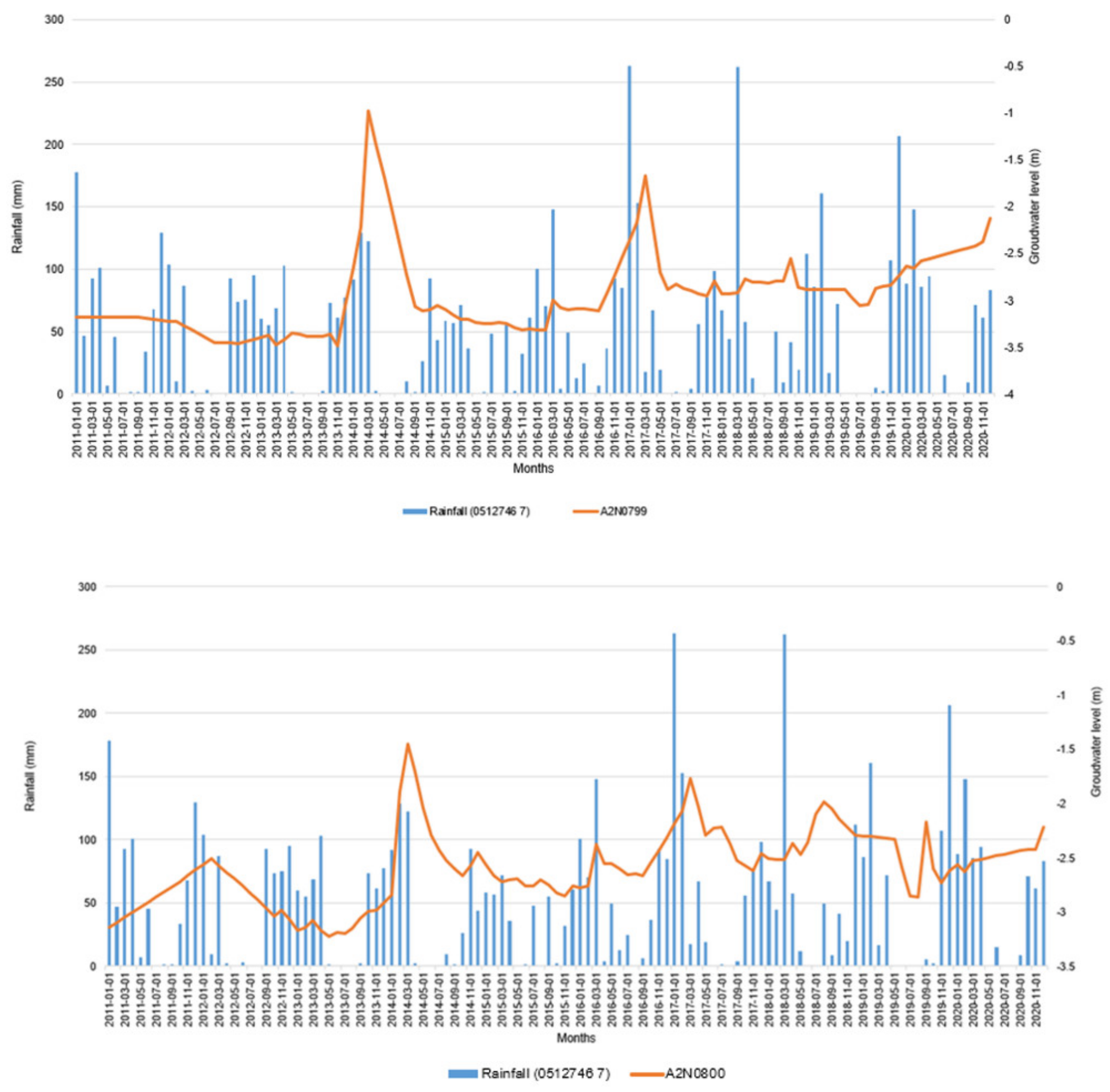
Two increasing trends were detected for groundwater station A2N0800 and A2N0799, making up 25% of the groundwater stations under study. As mentioned in the introduction, rainfall is a major input into the hydrogeological system and in this study, a significant multiple correlation coefficient, which was above 0.7, was obtained in all stations. The increasing trends can imply that there was generally higher rainfall than losses from the hydrogeological system in these two stations. The rainfall that occurred in early 2017, which according to Figure 4 is the maximum rainfall, may have served as a major contribution to this increasing trend.
Secondly, the two stations lie furthest from the Bloubankspruit river, and they are located close to each other and are at higher elevations compared to the other stations. The increase may be attributed to lower surface water and groundwater interchange when compared to the stations that lie closest to the Bloubankspruit river, because they may be losing water to the river during dry periods.
There were four stations that showed a decreasing trend, A2N0795, A2N0794, A2N0802 and A2N0805, amounting to 50% of the total groundwater stations under the study. The decreasing trends can be attributed to the low rainfall in 2015; according to Figure 5, 2015 recorded the lowest rainfall, of around 423 mm. Generally, lower rainfall was observed between 2012 and 2015, and it was below the mean annual rainfall for the study area, of around 600 mm to 800 mm [55]. There was also another dry hydrological year, 2018 to 2019, which could also be a contributing factor to the declining trend.
Groundwater can be a vital source of streamflow, particularly during droughts/dry seasons [64]. The shallow boreholes lying along the Bloubankspruit river may have lost water to the river during the drier hydrological years. Again, the variables of interests in this study are antecedent GWLs and rainfall, which gave a good (greater than 0.7) multiple correlation coefficient. Thus, the second factor that could be attributed to the declining trend may be the losses within the hydrogeological system, which are beyond the scope of this study.
The remaining 25% of stations did not indicate a trend: stations A2N0801 and A2N0806, shown in Figure 6. What is in common with these two stations is that they are located somewhere between the stations with increasing trends and those with decreasing trends. The cause of this could also be attributed to the abrupt climate change events that have occurred in the country during the past decade as well as the heterogeneity of the nature of hydrogeological systems.

3.3. Performance Evaluation of the Predictive Model

3.3.1. MSE and MAE

The MSE and MAE results for the calibration and validation models are presented in Figure 7 and Figure 8. The MSE values are in the range of 0.003 to 0.185, while the MAE values are from 0.04 to 0.345 in the calibration period. The station with the highest MSE and MAE values was station A2N0794, which was the station with the deepest water table among the stations, in the range of 23.4 m to 20.5 m below the ground. The station with the lowest MSE and MAE was A2N0801. Also, from Figure 7 the GB model had lower MSE and MAE values in all the stations when compared to the SVR model. Lower MSE and MAE imply good model performance.
Similarly, Figure 8 shows lower MSE and MAE values for the GB model in all the stations. The MSE values for the validation period range from 0.03 to 1.536, while the MAE values range from 0.12 to 1.188. Again, station A2N0794 had the highest MSE and MAE values, while station A2N0801 had the lowest MSE and MAE values.
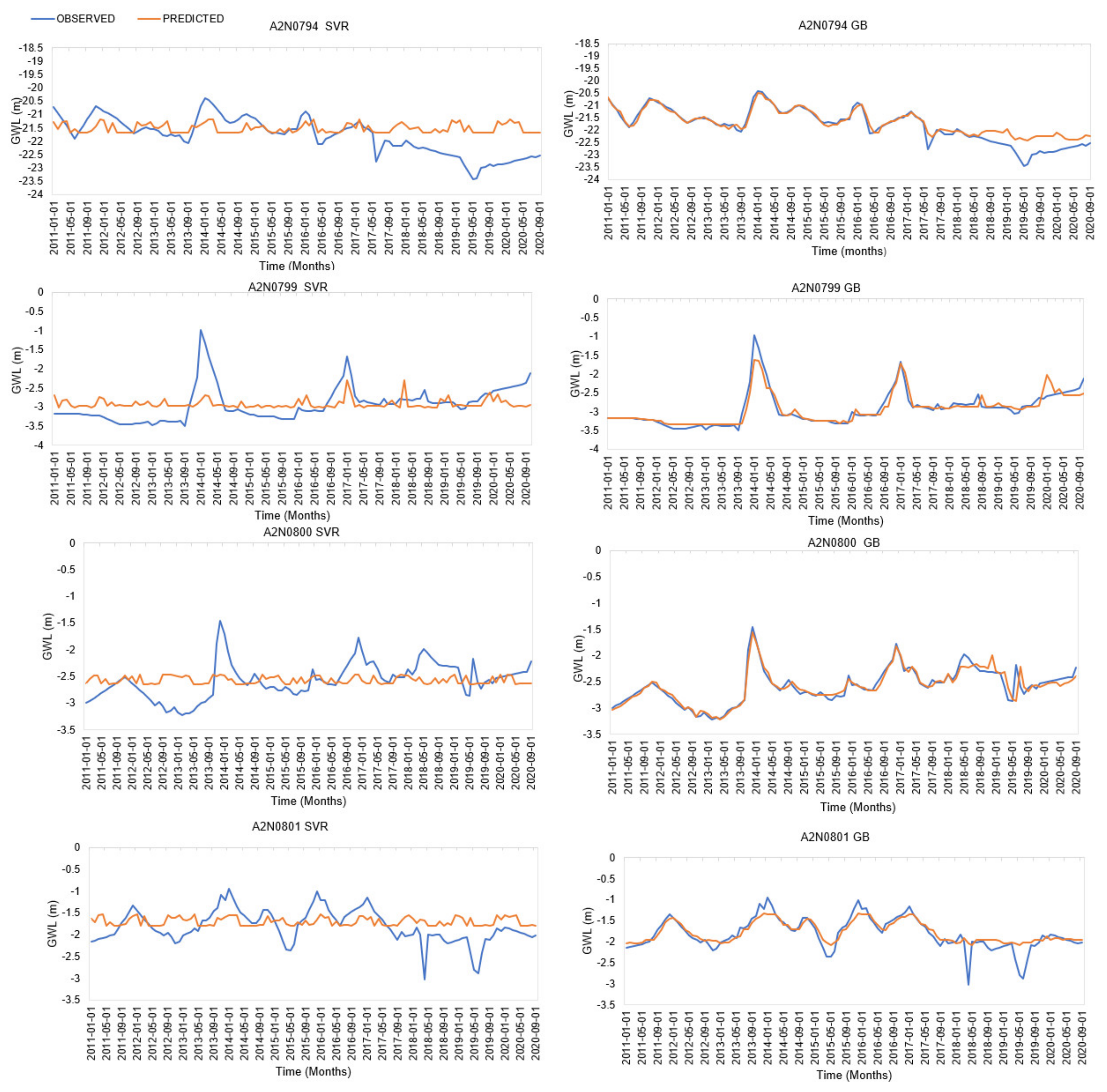
Both the GB and the SVR model reveal a better calibration model than a validation model, which could be attributed to the size of the dataset during the validation phase. In this particular study, around 75% of the data were used for calibration, while around 25% were used for validation. Figure 9 clearly shows that the GB model provides a better fit between the predicted and the observed GWLs during the calibration and the validation period of the model. What is also evident in Figure 9 is that the SVR prediction seems to agree with the trend of the observed data but fails to capture the low and the high values that are captured by the observed data. This failure to capture the low and the high values of the SVR model may be attributed to the input parameters, as the SVR is generally sensitive to input parameters [45]. However, based on Figure 9, the GB is able to capture the trend and closely agrees to the low and the high values depicted through the observed data. This concurs with some studies that have shown the robustness of GB against extreme values and abrupt inconsistencies [43,46,47].

3.3.2. Scatterplot Analysis

Figure 10 shows the scatterplots for the predicted and observed GWL for all four stations. High R2 values, which are between 0.7 and 1, reveal a good correlation between the predicted and observed GWL. R2 values for the GB model show a good performance of the model, ranging from 0.795 to 0.9, while the SVR model shows very poor R2 values at a range of 0.0018 to 0.1253. Again, findings obtained from the MAE and the MSE are supported by the scatterplots and the related R2 values. Again, the results agree with similar studies. For instance, Kanyama et al. [42] compared SVR, GB, ANN, Random Forest (RF) and Decision Trees (DT) in predicting GWLs. GB was the best model among the models, with R2 values above 0.7 in all the stations that were studied.
Sharafati et al. [36] also obtained accurate and consistent prediction results in assessing the use of GB for short-term and long-term GWL predictions.

4. Conclusions and Recommendations

In this study, a trend analysis over a study period from 2010 to 2020 was carried out and a GWL prediction model was derived. Trends and predictive models play a crucial role towards informing proactive decision making. Correlation analysis informed the choice of input variables in the predictive model. Multiple correlation analysis revealed coefficients greater than 0.7 in all the stations; ACF were also greater than 0.7, while the CCmax were the lowest among the correlation coefficients. The low CCmax were attributed to the lack of GWL measurements at a finer temporal resolution. The stations that were studied were generally shallow and thus shorter response times to rainfall were expected from these boreholes, but such data are not available. The multiple correlation coefficients showed that there is a relationship between the variables that were studied and informed the choice of the antecedent GWL and rainfall as input variables into the predictive model. The antecedent GWLs represented the hydrogeological aspect, while rainfall represented a climatic aspect. The correlation results also provided grounds to justify the GWL trends obtained using rainfall. Through trend analysis, it was deduced that 50% of the stations that were studied are undergoing a negative trend, 25% a positive trend and 25% of the stations do not indicate a trend. Thus, the negative trend was mainly attributed to low rainfall between 2012 and 2015, and the high surface-water–groundwater exchange that occurs in the stations that lie along the rivers, particularly when rainfall amounts are low. The positive trends were associated with higher rainfalls that took place around 2017. The 25% of no trend may be attributed to the heterogeneity that exists in the hydrogeological context.
Predictive models were developed, and the best predictive model was found to be the GB model with the lower MSE and MAE values and the higher R2 when compared to the SVR model. Therefore, based on projected rainfall and existing groundwater levels, future GWLs can be predicted using the GB model derived in this study area. What is unique about this study is that data-driven approaches were employed to depict the historical trends and in predictive modelling, while most of the studies in this study area focused on the physically based models. Furthermore, the processes of input variable selection through correlation analysis and GB were not computationally intensive.
The poor performance of the SVR methods could be improved by modifying the SVR model through combining the SVR with wavelet transform. Generally, the performance of both the models in the validation period was lower and could be improved by increasing the data size through increasing the temporal resolution of the input variable in the future. Due to the computational efficiency of the methods used in this study, their application is recommended in other aquifers.
The missing component of the envisioned groundwater management system that was not captured in this study, and which is quite important, is real-time data analysis. The next paper will thus look at the real-time groundwater management component. Real-time or near-real-time analysis will aid in improving rainfall–GWL cross-correlation coefficients and the accuracy of their lags, which will enhance the robustness of the predictive model.
The findings of this study, in light of climate change, imply that trends can be used for gaining insights into the long-term behaviour of GWLs as they indicate whether GWLs have been declining or increasing over time, while predictive modelling can aid in gaining insights into future GWLs conditions. Thus, information from the detected trends and predicted GWLs can be used in devising future groundwater utilization strategies through the application of real-time decision support systems. Consequently, this will aid in preserving groundwater resources when faced with climate-change-related disasters.

Author Contributions

Conceptualization, T.M.T.; Methodology, T.M.T.; Software, T.M.T.; Validation, T.M.T.; Formal analysis, T.M.T.; Investigation, T.M.T.; Resources, T.M.T., J.M.N. and T.O.O.; Writing—original draft, T.M.T.; Writing—review & editing, T.M.T., J.M.N., T.O.O. and S.S.R.; Visualization, T.M.T. and S.S.R.; Supervision, J.M.N., T.O.O. and S.S.R.; Project administration, J.M.N., T.O.O. and S.S.R.; Funding acquisition, J.M.N. All authors have read and agreed to the published version of the manuscript.

Funding

This research received no external funding.

Data Availability Statement

Not applicable.

Acknowledgments

The authors would like to thank the South African Weather Service and the Department of Water of Sanitation for providing the data used in this study.

Conflicts of Interest

The authors declare no conflict of interest.

References

  1. Ziervogel, G.; New, M.; Archer van Garderen, E.; Midgley, G.; Taylor, A.; Hamann, R.; Stuart-Hill, S.; Myers, J.; Warburton, M. Climate change impacts and adaptation in South Africa. Wiley Interdiscip. Rev. Clim. Change 2014, 5, 605–620. [Google Scholar] [CrossRef]
  2. IPCC. Climate Change 2014: Impacts, Adaptation, and Vulnerability. Part A: Global and Sectoral Aspects. Contribution of Working Group II to the Fifth Assessment Report of the Intergovernmental Panel on Climate Change; Intergovernmental Panel on Climate Change: New York, NY, USA, 2014. [Google Scholar]
  3. Mishra, A.K.; Singh, V.P. A review of drought concepts. J. Hydrol. 2010, 391, 202–216. [Google Scholar] [CrossRef]
  4. Wanders, N.; Wada, Y.; Van Lanen, H.A.J. Global hydrological droughts in the 21st century under a changing hydrological regime. Earth Syst. Dyn. 2015, 6, 1–15. [Google Scholar] [CrossRef]
  5. Prodhan, F.A.; Zhang, J.; Pangali Sharma, T.P.; Nanzad, L.; Zhang, D.; Seka, A.M.; Ahmed, N.; Hasan, S.S.; Hoque, M.Z.; Mohana, H.P. Projection of future drought and its impact on simulated crop yield over South Asia using ensemble machine learning approach. Sci. Total Environ. 2022, 807, 151029. [Google Scholar] [CrossRef]
  6. Dilawar, A.; Chen, B.; Arshad, A.; Guo, L.; Ehsan, M.I.; Hussain, Y.; Kayiranga, A.; Measho, S.; Zhang, H.; Wang, F.; et al. Towards understanding variability in droughts in response to extreme climate conditions over the different agro-ecological zones of Pakistan. Sustainability 2021, 13, 6910. [Google Scholar] [CrossRef]
  7. Centre for Research on the Epidemiology of Disasters. Disasters in Numbers 2022; CRED: Brussels, Belgium, 2023. [Google Scholar]
  8. Schreiner, B.G.; Mungatana, E.D.; Baleta, H. Impacts of Drought Induced Water Shortages in South Africa: Economic Analysis Report to the Water Research Commission. 2018. Available online: www.wrc.org.za (accessed on 15 February 2023).
  9. Archer, E.; du Toit, J.; Engelbrecht, C.; Hoffman, M.T.; Landman, W.; Malherbe, J.; Stern, M. The 2015-19 multi year drought in the Eastern Cape, South Africa: It’s evolution and impacts on agriculture. J. Arid Environ. 2022, 196, 104630. [Google Scholar] [CrossRef]
  10. Holmes, M.; Campbell, E.E.; De Wit, M.; Taylor, J.C. South African Journal of Botany The impact of drought in the Karoo—Revisiting diatoms as water quality indicators in the upper reaches of the Great Fish River, Eastern Cape, South Africa. S. Afr. J. Bot. 2022, 149, 502–510. [Google Scholar] [CrossRef]
  11. Olanrewaju, C.C.; Reddy, M. Assessment and prediction of flood hazards using standardized precipitation index—A case study of eThekwini metropolitan area. J. Flood Risk Manag. 2022, 15, e12788. [Google Scholar] [CrossRef]
  12. Bopape, M.J.M.; Sebego, E.; Ndarana, T.; Maseko, B.; Netshilema, M.; Gijben, M.; Landman, S.; Phaduli, E.; Rambuwani, G.; van Hemert, L.; et al. Evaluating south african weather service information on idai tropical cyclone and kwazulu-natal flood events. S. Afr. J. Sci. 2021, 117, 1–13. [Google Scholar] [CrossRef]
  13. Madzivhandila Thanyani, S.; Maserumule, M.H. The Irony of A “Fire Fighting” Approach Towards Natural Hazards in South Africa: Lessons from Flooding Disaster in KwaZulu-Natal. J. Public Adm. 2022, 57, 191–194. [Google Scholar]
  14. Chandrasekara, S.S.K.; Kwon, H.H.; Vithanage, M.; Obeysekera, J.; Kim, T.W. Drought in south Asia: A review of drought assessment and prediction in south Asian countries. Atmosphere 2021, 12, 369. [Google Scholar] [CrossRef]
  15. Hussain, M.; Butt, A.R.; Uzma, F.; Ahmed, R.; Irshad, S.; Rehman, A.; Yousaf, B. A comprehensive review of climate change impacts, adaptation, and mitigation on environmental and natural calamities in Pakistan. Environ. Monit. Assess. 2020, 192, 48. [Google Scholar] [CrossRef] [PubMed]
  16. Quesada-Román, A.; Villalobos-Portilla, E.; Campos-Durán, D. Hydrometeorological disasters in urban areas of Costa Rica, Central America. Environ. Hazards 2020, 20, 264–278. [Google Scholar] [CrossRef]
  17. Department of Water Affairs. Groundwater Strategy 2010; Department of Water and Sanitation: Pretoria, South Africa, 2010.
  18. Pietersen, K.; Beekman, H.E.; Holland, M. South African Groundwater Governance Case Study; WRC: Pretoria, South Africa, 2011. [Google Scholar]
  19. Bloomfield, J.P.; Allen, D.J.; Griffiths, K.J. Examining geological controls on baseflow index (BFI) using regression analysis: An illustration from the Thames Basin, UK. J. Hydrol. 2009, 373, 164–176. [Google Scholar] [CrossRef]
  20. Zomlot, Z.; Verbeiren, B.; Huysmans, M.; Batelaan, O. Spatial distribution of groundwater recharge and base flow: Assessment of controlling factors. J. Hydrol. Reg. Stud. 2015, 4, 349–368. [Google Scholar] [CrossRef]
  21. Mohan, C.; Western, A.W.; Wei, Y.; Saft, M. Predicting groundwater recharge for varying land cover and climate conditions—A global meta-study. Hydrol. Earth Syst. Sci. 2018, 22, 2689–2703. [Google Scholar] [CrossRef]
  22. Keese, K.E.; Scanlon, B.R.; Reedy, R.C. Assessing controls on diffuse groundwater recharge using unsaturated flow modeling. Water Resour. Res. 2005, 41, 1–12. [Google Scholar] [CrossRef]
  23. Sun, H.; Cornish, P.S. Estimating shallow groundwater recharge in the headwaters of the Liverpool Plains using SWAT. Hydrol. Process. 2005, 19, 795–807. [Google Scholar] [CrossRef]
  24. Alfaro, P.; Liesch, T.; Goldscheider, N. Modelling groundwater over-extraction in the southern Jordan Valley with scarce data. Hydrogeol. J. 2017, 25, 1319–1340. [Google Scholar] [CrossRef]
  25. Oke, S.A.; Fourie, F. Guidelines to groundwater vulnerability mapping for Sub-Saharan Africa. Groundw. Sustain. Dev. 2017, 5, 168–177. [Google Scholar] [CrossRef]
  26. Sahoo, M.; Kasot, A.; Dhar, A.; Kar, A. On Predictability of Groundwater Level in Shallow Wells Using Satellite Observations. Water Resour. Manag. 2018, 32, 1225–1244. [Google Scholar] [CrossRef]
  27. Castellazzi, P.; Longuevergne, L.; Martel, R.; Rivera, A.; Brouard, C.; Chaussard, E. Quantitative mapping of groundwater depletion at the water management scale using a combined GRACE/InSAR approach. Remote Sens. Environ. 2018, 205, 408–418. [Google Scholar] [CrossRef]
  28. Lyazidi, R.; Hessane, M.A.; Moutei, J.F.; Bahir, M. Developing a methodology for estimating the groundwater levels of coastal aquifers in the Gareb-Bourag plains, Morocco embedding the visual MODFLOW techniques in groundwater modeling system. Groundw. Sustain. Dev. 2020, 11, 100471. [Google Scholar] [CrossRef]
  29. Ostad-Ali-Askari, K.; Ghorbanizadeh Kharazi, H.; Shayannejad, M.; Zareian, M.J. Effect of management strategies on reducing negative impacts of climate change on water resources of the Isfahan–Borkhar aquifer using MODFLOW. River Res. Appl. 2019, 35, 611–631. [Google Scholar] [CrossRef]
  30. Ibrahem, A.; Osman, A.; Najah, A.; Fai, M.; Feng, Y.; El-Shafie, A. Extreme gradient boosting (Xgboost) model to predict the groundwater levels in Selangor Malaysia. Ain Shams Eng. J. 2021, 12, 1545–1556. [Google Scholar] [CrossRef]
  31. Malekzadeh, M.; Kardar, S.; Shabanlou, S. Simulation of groundwater level using MODFLOW, extreme learning machine and Wavelet-Extreme Learning Machine models. Groundw. Sustain. Dev. 2019, 9, 100279. [Google Scholar] [CrossRef]
  32. Zeydalinejad, N. Artificial neural networks vis-à-vis MODFLOW in the simulation of groundwater: A review. Model. Earth Syst. Environ. 2022, 8, 2911–2932. [Google Scholar] [CrossRef]
  33. Rezaei, M.; Mousavi, S.F.; Moridi, A.; Eshaghi Gordji, M.; Karami, H. A new hybrid framework based on integration of optimization algorithms and numerical method for estimating monthly groundwater level. Arab. J. Geosci. 2021, 14, 994. [Google Scholar] [CrossRef]
  34. Ahmadi, A.; Olyaei, M.; Heydari, Z.; Emami, M.; Zeynolabedin, A.; Ghomlaghi, A.; Daccache, A.; Fogg, G.E.; Sadegh, M. Groundwater Level Modeling with Machine Learning: A Systematic Review and Meta-Analysis. Water 2022, 14, 949. [Google Scholar] [CrossRef]
  35. Hussein, E.A.; Thron, C.; Ghaziasgar, M.; Bagula, A.; Vaccari, M. Groundwater prediction using machine-learning tools. Algorithms 2020, 13, 300. [Google Scholar] [CrossRef]
  36. Sharafati, A.; Asadollah, S.B.H.S.; Neshat, A. A new artificial intelligence strategy for predicting the groundwater level over the Rafsanjan aquifer in Iran. J. Hydrol. 2020, 591, 125468. [Google Scholar] [CrossRef]
  37. Murdoch, W.J.; Singh, C.; Kumbier, K.; Abbasi-Asl, R.; Yu, B. Definitions, methods, and applications in interpretable machine learning. Proc. Natl. Acad. Sci. USA 2019, 116, 22071–22080. [Google Scholar] [CrossRef] [PubMed]
  38. Aderemi, B.A.; Olwal, T.O.; Ndambuki, J.M.; Rwanga, S.S. Groundwater levels forecasting using machine learning models: A case study of the groundwater region 10 at Karst Belt, South Africa. Syst. Soft Comput. 2023, 5, 200049. [Google Scholar] [CrossRef]
  39. Osman, A.I.A.; Ahmed, A.N.; Huang, Y.F.; Kumar, P.; Birima, A.H.; Sherif, M.; Sefelnasr, A.; Ebraheemand, A.A.; El-Shafie, A. Past, Present and Perspective Methodology for Groundwater Modeling-Based Machine Learning Approaches. Arch. Comput. Methods Eng. 2022, 29, 3843–3859. [Google Scholar] [CrossRef]
  40. Wei, A.; Chen, Y.; Li, D.; Zhang, X.; Wu, T.; Li, H. Prediction of groundwater level using the hybrid model combining wavelet transform and machine learning algorithms. Earth Sci. Inform. 2022, 15, 1951–1962. [Google Scholar] [CrossRef]
  41. Ouali, L.; Kabiri, L.; Namous, M.; Hssaisoune, M.; Abdelrahman, K.; Fnais, M.S.; Kabiri, H.; El Hafyani, M.; Oubaassine, H.; Arioua, A.; et al. Spatial Prediction of Groundwater Withdrawal Potential Using Shallow, Hybrid, and Deep Learning Algorithms in the Toudgha Oasis, Southeast Morocco. Sustainability 2023, 15, 3874. [Google Scholar] [CrossRef]
  42. Kanyama, Y.; Ajoodha, R.; Seyler, H.; Makondo, N.; Tutu, H. Application of machine learning techniques in forecasting groundwater levels in the Grootfontein aquifer. In Proceedings of the 2020 2nd International Multidisciplinary Information Technology and Engineering Conference (IMITEC 2020), Kimberley, South Africa, 25–27 November 2020. [Google Scholar] [CrossRef]
  43. Zhang, Y.; Haghani, A. A gradient boosting method to improve travel time prediction. Transp. Res. Part C 2015, 58, 308–324. [Google Scholar] [CrossRef]
  44. Jafari, H.; Rajaee, T.; Kisi, O. Improved Water Quality Prediction with Hybrid Wavelet-Genetic Programming Model and Shannon Entropy. Nat. Resour. Res. 2020, 29, 3819–3840. [Google Scholar] [CrossRef]
  45. He, X.; Luo, J.; Li, P.; Zuo, G.; Xie, J. A Hybrid Model Based on Variational Mode Decomposition and Gradient Boosting Regression Tree for Monthly Runoff Forecasting. Water Resour. Manag. 2020, 34, 865–884. [Google Scholar] [CrossRef]
  46. An, R.; Tong, Z.; Ding, Y.; Tan, B.; Wu, Z.; Xiong, Q.; Liu, Y. Examining non-linear built environment effects on injurious traffic collisions: A gradient boosting decision tree analysis. J. Transp. Health 2022, 24, 101296. [Google Scholar] [CrossRef]
  47. Olinsky, A.; Kennedy, B.B. Assessing Gradient Boosting in the Reduction of Misclassification Error in the Prediction of Success for Actuarial Majors. Case Stud. Bus. Ind. Gov. Stat. 2012, 5, 12–16. [Google Scholar]
  48. Maier, H.R.; Dandy, G.C. Neural networks for the prediction and forecasting of water resources variables: A review of modelling issues and applications. Environ. Model. Softw. 2000, 15, 101–124. [Google Scholar] [CrossRef]
  49. Tao, H.; Majeed, M.; Abdulameer, H.; Zounemat, M.; Heddam, S.; Kim, S.; Oleiwi, S.; Leong, M.; Sa, Z.; Danandeh, A.; et al. Neurocomputing Groundwater level prediction using machine learning models: A comprehensive review. Neurocomputing 2022, 489, 271–308. [Google Scholar] [CrossRef]
  50. Derbela, M.; Nouiri, I. Intelligent approach to predict future groundwater level based on artificial neural networks (ANN). Euro-Mediterr. J. Environ. Integr. 2020, 5, 51. [Google Scholar] [CrossRef]
  51. Yoon, H.; Hyun, Y.; Ha, K.; Lee, K.; Kim, G. Computers & Geosciences A method to improve the stability and accuracy of ANN- and SVM-based time series models for long-term groundwater level predictions. Comput. Geosci. 2016, 90, 144–155. [Google Scholar] [CrossRef]
  52. Gaffoor, Z.; Gritzman, A.; Pietersen, K.; Jovanovic, N.; Bagula, A.; Kanyerere, T. An autoregressive machine learning approach to forecast high-resolution groundwater-level anomalies in the Ramotswa/North West/Gauteng dolomite aquifers of Southern Africa. Hydrogeol. J. 2022, 30, 575–600. [Google Scholar] [CrossRef]
  53. Condon, L.E.; Kollet, S.; Bierkens, M.F.P.; Fogg, G.E.; Maxwell, R.M.; Hill, M.C.; Fransen, H.J.H.; Verhoef, A.; Van Loon, A.F.; Sulis, M.; et al. Global Groundwater Modeling and Monitoring: Opportunities and Challenges. Water Resour. Res. 2021, 57, e2020WR029500. [Google Scholar] [CrossRef]
  54. DWAF. Crocodile River (West) and Marico Water Management Area: Internal Strategic Perspective of the Crocodile River (West) Catchment; Department of Water Affairs and Forestry of South Africa: Pretoria, South Africa, 2004; Volume 3, p. 160.
  55. Schulze, R.E. A 2011 Perspective on Climate Change and The South African Water Sector. 2012. Available online: http://www.wrc.org.za/wp-content/uploads/mdocs/TT518-12.pdf (accessed on 15 February 2023).
  56. Abiye, T.A.; Mengistu, H.; Masindi, K.; Demlie, M. Surface Water and Groundwater Interaction in the Upper Crocodile River Basin, Johanesburg, South Africa: Environmental Isotope Approach. S. Afr. J. Geol. 2015, 118, 109–118. [Google Scholar] [CrossRef]
  57. Meyer, M. Hydrogeology of Groundwater Region 10: The Karst Belt (WRC Project No. K5/1916); WRC: Pretoria, South Africa, 2014. [Google Scholar]
  58. Hadi, A.S.; Imon, A.H.M.R.; Werner, M. Detection of outliers. Wiley Interdiscip. Rev. Comput. Stat. 2009, 1, 57–70. [Google Scholar] [CrossRef]
  59. Dovoedo, Y.H.; Chakraborti, S. Computation Boxplot-Based Outlier Detection for the Location-Scale Family Boxplot-Based Outlier Detection for the Location-Scale Family. Commun. Stat.-Simul. Comput. 2015, 44, 1492–1513. [Google Scholar] [CrossRef]
  60. Mushtaq, Z.; Ramzan, M.F.; Ali, S.; Baseer, S.; Samad, A.; Husnain, M. Voting Classification-Based Diabetes Mellitus Prediction Using Hypertuned Machine-Learning Techniques. Mob. Inf. Syst. 2022, 2022, 6521532. [Google Scholar] [CrossRef]
  61. Denić-Jukić, V.; Lozić, A.; Jukić, D. An application of correlation and spectral analysis in hydrological study of neighboring karst springs. Water 2020, 12, 3570. [Google Scholar] [CrossRef]
  62. Rahmani, F.; Fattahi, M.H. A multifractal cross-correlation investigation into sensitivity and dependence of meteorological and hydrological droughts on precipitation and temperature. Nat. Hazards 2021, 109, 2197–2219. [Google Scholar] [CrossRef]
  63. Seo, S.B.; Das Bhowmik, R.; Sankarasubramanian, A.; Mahinthakumar, G.; Kumar, M. The role of cross-correlation between precipitation and temperature in basin-scale simulations of hydrologic variables. J. Hydrol. 2019, 570, 304–314. [Google Scholar] [CrossRef]
  64. Valois, R.; MacDonell, S.; Núñez Cobo, J.H.; Maureira-Cortés, H. Groundwater level trends and recharge event characterization using historical observed data in semi-arid Chile. Hydrol. Sci. J. 2020, 65, 597–609. [Google Scholar] [CrossRef]
  65. Mann, H.B. Non-Parametric Test Against Trend. Econometrica 1945, 13, 245–259. Available online: http://www.economist.com/node/18330371?story%7B_%7Did=18330371 (accessed on 15 February 2023). [CrossRef]
  66. Mathivha, F.I.; Nkosi, M.; Mutoti, M.I. Evaluating the relationship between hydrological extremes and groundwater in Luvuvhu River Catchment, South Africa. J. Hydrol. Reg. Stud. 2021, 37, 100897. [Google Scholar] [CrossRef]
  67. Gyamfi, C.; Ndambuki, J.M.; Salim, R.W. A Historical Analysis of Rainfall Trend in the Olifants Basin in South Africa. Earth Sci. Res. 2016, 5, 129. [Google Scholar] [CrossRef]
  68. Alhaji, U.U.; Yusuf, A.S.; Edet, C.O.; Oche, C.O.; Agbo, E.P. Trend Analysis of Temperature in Gombe State Using Mann Kendall Trend Test. J. Sci. Res. Rep. 2018, 20, 1–9. [Google Scholar] [CrossRef]
  69. Géron, A. Hands-on Machine Learning whith Scikit-Learing, Keras and Tensorfow; O’Reilly Media: Sebastopol, CA, USA, 2019; ISBN 978-1-492-03264-9. [Google Scholar]
  70. Yu, P.; Chen, S.; Chang, I. Support vector regression for real-time flood stage forecasting. J. Hydrol. 2006, 328, 704–716. [Google Scholar] [CrossRef]
  71. Granata, F.; Gargano, R.; Marinis, G. De Support Vector Regression for Rainfall-Runoff Modeling in Urban Drainage: A Comparison with the EPA’ s Storm Water Management Model. Water 2016, 8, 69. [Google Scholar] [CrossRef]
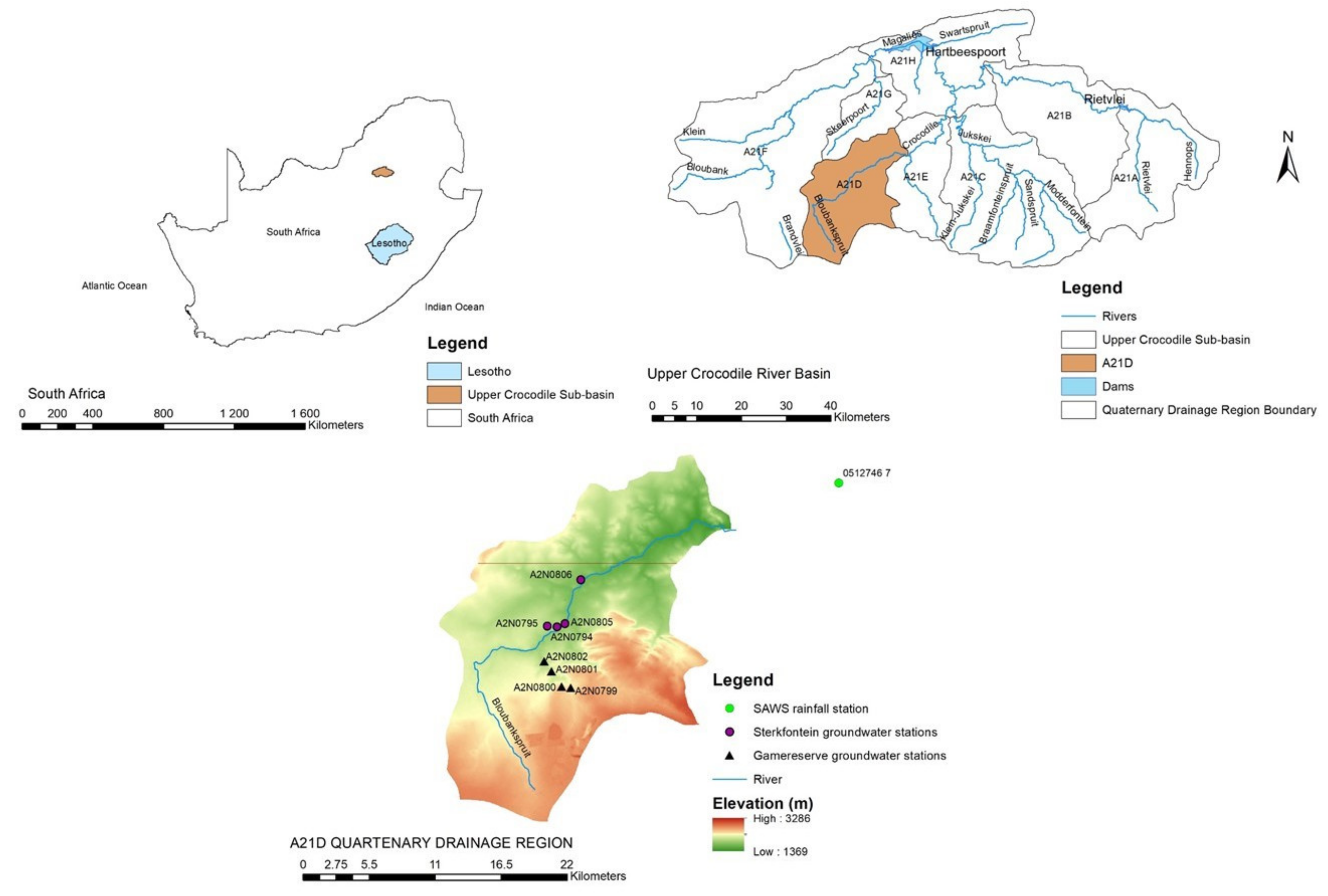
Figure 1. Study area.
Water 15 03025 g001
Figure 2. Support vector regression [30].
Water 15 03025 g002
Figure 3. Workflow diagram.
Water 15 03025 g003
Figure 4. Groundwater stations with increasing MK trend.
Water 15 03025 g004
Figure 5. Groundwater stations with decreasing MK trend.
Water 15 03025 g005
Figure 6. Groundwater stations with no trend.
Water 15 03025 g006
Figure 7. The MSE and MAE values for calibration.
Water 15 03025 g007
Figure 8. The MSE and MAE values for validation.
Water 15 03025 g008
Figure 9. Observed and Predicted GWLs in the calibration and validation periods.
Water 15 03025 g009
Figure 10. Scatterplots for the predicted versus observed GWL.
Water 15 03025 g010
Table 1. Groundwater stations selected for the analysis.
Station NumberLatitudeLongitudeStart DateQuaternary
A2N0794−26.04827.7091 September 2008A21D
A2N0795−26.04727.7021 September 2008A21D
A2N0799−26.09327.7191 September 2008A21D
A2N0800−26.09227.7121 September 2008A21D
A2N0801−26.08127.7051 September 2008A21D
A2N0802−26.07327.6991 September 2008A21D
A2N0805−26.04527.7151 September 2008A21D
A2N0806−26.01227.7271 September 2008A21D
Table 2. Correlations and selected lags for the predictive model.
Input VariableRGWLR/GWL
StationLag (Month) CCmaxLag (Month) ACFMultiple Correlation Coefficient
A2N079430.14510.940.955
A2N079920.28810.8920.91
A2N080020.210.8650.875
A2N080110.23910.8510.858
Disclaimer/Publisher’s Note: The statements, opinions and data contained in all publications are solely those of the individual author(s) and contributor(s) and not of MDPI and/or the editor(s). MDPI and/or the editor(s) disclaim responsibility for any injury to people or property resulting from any ideas, methods, instructions or products referred to in the content.