A Comparison of Saturated Hydraulic Conductivity (Ksat) Estimations from Pedotransfer Functions (PTFs) and Field Observations in Riparian Seasonal Wetlands

Abstract

Accurate saturated hydraulic conductivity (Ksat) predictions are critical for precise water flow estimations. Pedotransfer functions (PTFs) have been used to estimate Ksat based on soil structural and textural properties. However, PTF accuracy must be validated with observed Ksat values to improve confidence in model predictions. A study was conducted in the seasonal wetlands of a representative mixed land-use watershed in West Virginia (WV), USA. The observed data included soil characteristics and observed piezometric Ksat using slug tests. Soil texture was predominantly sandy, and the observed average Ksat ranged from 35.90 to 169.64 m/d. The average bulk dry density (bdry) increased, while porosity and volumetric water content decreased significantly with a depth to 45 cm (p < 0.05). The degree of saturation varied significantly between monitoring sites (p < 0.05). A Pearson correlation matrix and Principal Component Analysis (PCA) revealed that Ksat was more connected to soil textural properties, specifically clay. Single parameter PTFs that estimated Ksat as a function of clay content performed better (ME = −90.19 m/d, RMSE = 102.87 m/d) than the PTFs that used silt or sand percentages (ME= −96.86 m/d, RMSE = 108.77). However, all five PTFs predicted Ksat with low accuracy (RMSE > 100 m/d), emphasizing the need to calibrate existing PTFs with observed data or develop site-specific PTFs. These results provide valuable insights into Ksat estimation in riparian wetlands of mixed land-use watersheds and are a helpful reference for land managers and future work.

1. Introduction

Saturated hydraulic conductivity (Ksat) relates water transport to hydraulic gradients [1] and influences the relative magnitude of local water balance components, such as infiltration, soil moisture, stream discharge, and groundwater flow [2,3,4,5,6]. Accurate Ksat estimates are essential for predicting flow dynamics and pollutant loading and making effective watershed management decisions. Ksat can be directly measured in the field or laboratory using various methods, including pump tests, slug tests, borehole flowmeter tests, and hydraulic tomography [7,8,9]. However, for large-scale landscape and modeling applications, direct measurements of Ksat are often impractical, time-consuming, and costly [3,6,10].

Pedotransfer Functions (PTFs) are an acceptable alternative to obtaining Ksat estimates when direct (observed) Ksat measurements are impractical [3,6,8,11,12]. PTFs are empirical models used to estimate Ksat from relatively easily measured soil physical properties such as soil bulk density, porosity, effective grain size diameter (GSD), and soil texture [3,10,11,12,13,14]. Soil texture represents sand, silt, and clay particle size fractions and is a reliable predictor of Ksat [3,4,13]. Puckett et al. [11] suggested that Ksat highly correlates to soil clay percentage (correlation coefficient 0.77). Substantial improvements in PTF estimations using soil texture are also possible with the inclusion of bulk density [3]. Additionally, PTFs that integrate GSD result in more accurate Ksat estimates than PTFs based on soil texture alone, as soil permeability and transmissive properties are quantified with greater confidence using GSD [15]. However, such models require additional analysis, and GSD data are often not as readily available [8,15,16].

PTFs require a wide range of soil physical characteristics to generate accurate estimations of Ksat [12]. Therefore, it is essential to understand the relationship between soil properties and Ksat to choose an appropriate PTF [17]. Previous researchers used the Pearson correlation matrix and Principal Component Analysis (PCA) to identify the strength and relationship of soil properties with Ksat [17,18,19,20,21]. For example, Gamie and De Smedt [19] analyzed the relationship between Ksat and soil properties in desert soils of Egypt and showed that soil structure had a stronger correlation with Ksat than soil texture. Similarly, Wang et al. [20] used Pearson correlation and PCA to identify closely correlated soil factors with Ksat and determine the regional distribution of Ksat in loess soils of China. In addition, Zuo and He [17] used PCA to perform an exploratory factor analysis for ten soil properties and later developed a new PTF using PCA outputs.

Despite the method yielding a relatively quick and inexpensive determination of Ksat, PTFs often do not include the spatial and temporal variability of soil water movement related to land use, land cover, and vegetation [22,23,24,25]. Previous studies showed that the reliability of PTFs is often limited in regions with similar soil properties and land-use history [17,24,25,26]. Lim et al. [25] determined the usefulness of six PTFs for Ksat prediction in forested soil of South Korea and concluded that observed Ksat was 10 times larger than Ksat estimated by PTFs. Similarly, Petryk et al. [26] analyzed the predictive accuracy of 15 PTFs in highly eroded loess soil samples and suggested a need to develop PTFs using local soil data. Duan et al. [22] compared observed Ksat versus estimated Ksat using three PTFs in Texas grassed soils. The authors concluded that all the PTFs provided estimations of Ksat with limited success and relatively large error (Root Mean Square Error; RMSE > 100). Differences were attributed to soil physical properties being different in lawn soils with healthy growing grass relative to agricultural topsoil. The Duan et al. [22] results differed from those of Gootman et al. [8]. Gootman et al. [8] analyzed the performance of five PTFs in the Chesapeake Bay Watershed of the eastern United States. The authors concluded that four out of five PTFs predicted Ksat with lower error (RMSE < 5). The Jabro PTF overestimated Ksat and had a higher error range (RMSE = 63.28) attributable to silt-dominated textures and was not suitable for soils with higher sand content (92%) [8].

While previous studies have validated PTFs across different land-use practices [8,22,25], there is a notable gap in validating and comparing these functions in seasonal riparian wetlands of mixed land-use watersheds, highlighting a need for future research. The relevance of this research extends beyond understanding the predictive accuracy of PTFs. Ksat is also a highly sensitive parameter in surface and subsurface flow prediction models such as SWAT, HYDRUS, and MODFLOW. It therefore serves a crucial role in streamflow and groundwater flow simulations [27,28,29,30]. Investigations must be undertaken that will ultimately increase confidence in estimated Ksat values for water flow dynamics and solute transport predictions [30,31] and guide model developers in improving model-predicted Ksat values.

The overarching objective of this research was to address the knowledge gap noted above by comparing PTF-estimated Ksat values with observed Ksat in seasonal riparian wetlands of a mixed land-use watershed in West Virginia (WV), USA. Sub-objectives included (a) collecting observed Ksat values using piezometric slug tests, (b) analyzing soil structural and textural properties from collected soil cores, (c) selecting appropriate PTFs by investigating the correlation and interrelationships of soil properties with Ksat, and (d) statistically comparing estimated Ksat values versus observed Ksat values. The results provide insights into the accuracy of PTFs and contribute to improving Ksat estimation in surface and subsurface flow prediction models.

2. Materials and Methods

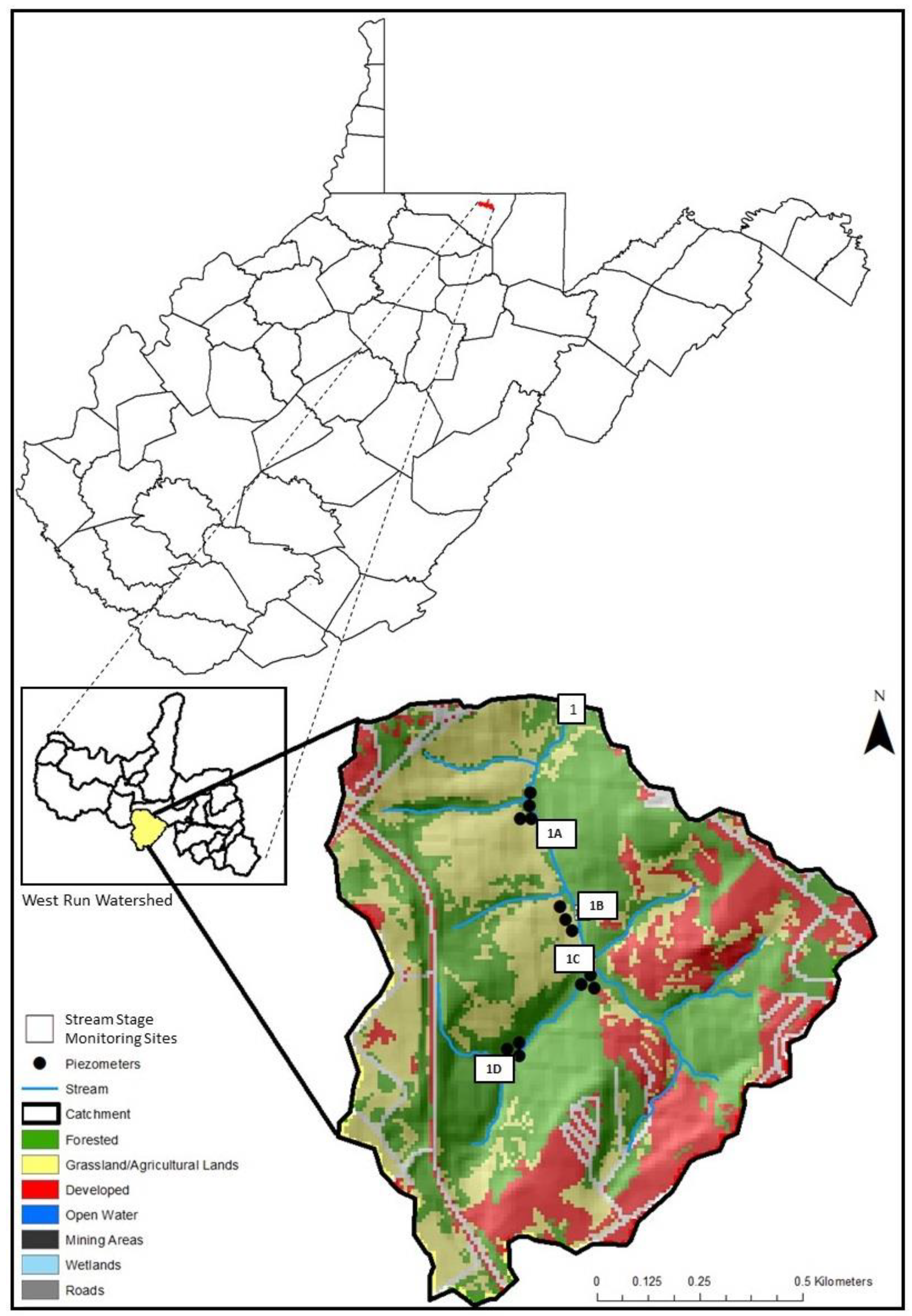
2.1. Site Descriptions

This study was conducted in seasonal riparian wetlands of a reach in the mixed land-use West Run Watershed (WRW) located in northeastern Morgantown, West Virginia (WV) (Figure 1). The study reach is a second-order stream that drains into the third-order West Run Creek, a Monongahela River tributary [32,33]. The watershed has a relatively uniform distribution of mixed development (31.77%), agriculture (33.72%), and forest areas (34.51%) [32], and is therefore classified as a mixed land use catchment. This investigation included five stream stage monitoring sites designated 1, 1A, 1B, 1C, and 1D. All monitoring sites except for 1 (located at the confluence with West Run Creek) were equipped with nested piezometer arrays. 1A had four nested piezometers, and 1B, 1C, and 1D each had three piezometers. As a result, the reach is instrumented with five stilling wells and thirteen piezometers in total (Figure 1).

Monitoring site soils were primarily Lobdell–Holly silt loam, with smaller portions of Clarksburg silt loam and Buchanan–Ernest very stony soil [34]. Lobdell–Holly silt loam is characterized by moderate permeability (0.6–2.0 in), allowing for slow runoff, while the Clarksburg silt loam and Buchanan–Ernest stony soils have low permeability (0.06–0.20 in) and rapid runoff [34]. Soils are further characterized by hydraulic conductivity (Ksat) of 0.78 m/d, with a dry bulk density of 1.3–1.43 g/cm³, according to the Natural Resources Conservation Service (NRCS) [35]. The NRCS estimates Ksat using textural triangle diagrams based on the soil texture, structure, and relative bulk density (low, medium, high) or by direct measurements using various methods, such as permeameters, double ring infiltrometers, and amoozemeters [36]. The soil texture in the study reach was previously estimated to be primarily silt, silty loam, or silty clay loam, with 19–25% sand, 60% silt, 15–21% clay, and 2–11% pebble [35].

In the study reach, rising and falling head slug tests were performed in piezometers to obtain observed measurements of Ksat. Additionally, soil cores were collected from two depths (0–5 cm and 40–45 cm) to analyze dry bulk density, porosity, degree of saturation, and volumetric water content. Particle size fractionations were performed on the dried soil samples using sieve analysis to determine the sand%, silt%, and clay%.

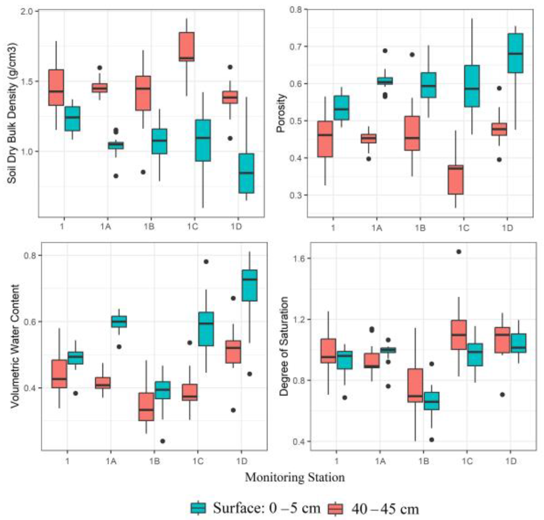
2.2. Soil Structural Characteristics

Soil cores were collected using 4 m × 4 m grids, resulting in 16 equidistant sampling points in the approximate piezometer cluster center for 1A to 1D. For site 1, the soil sample was collected approximately 2 m from the stream gauge site. At each sampling point, soil cores were collected from 2 depths: 0–5 cm and 40–45 cm. Soil samples were collected using the soil core method [37] by driving a cylindrical metal sampler into the soil of known depth. After transporting soil cores to the laboratory, soil samples were weighed and oven dried at 105 °C for 24 to 48 h [8,37]. Dry soil sample mass was recorded after the oven-dried sample was cooled to room temperature. Each soil core was processed, and the following soil characteristics [37,38,39] were calculated:

$$\mathrm{bdry}=\frac{\mathrm{Ms}}{\mathrm{Vt}}$$

(1)

$$\mathrm{Porosity}=\frac{\mathrm{Vf}}{\mathrm{Vt}}$$

(2)

$$\mathrm{VWC}=\frac{\mathrm{Vw}}{\mathrm{Vt}}$$

(3)

$$\mathrm{Degree} \mathrm{of} \mathrm{saturation}=\frac{\mathrm{Vw}}{\mathrm{Vf}}=\frac{\mathrm{VWC}}{\mathrm{Porosity}}$$

(4)

where bdry (g/cm³) is the soil dry bulk density, VWC (unitless) is the volumetric water content, Ms (g) is the mass of soil core solids, Vf (g) is the volume of soil core pore space, Vw (g) is the volume of water, and Vt (g) is the total soil core volume.

A two-way ANOVA was performed to test whether soil characteristics differed significantly between monitoring sites and by depth [8,40,41]. Two-way ANOVA was followed by a Tukey–Kramer honest significant difference (HSD) test [8,40] for significant differences (CI = 95%, p < 0.05) in soil characteristics in all possible combinations of depth and monitoring sites. All statistical analyses were performed using R statistical programming software [42].

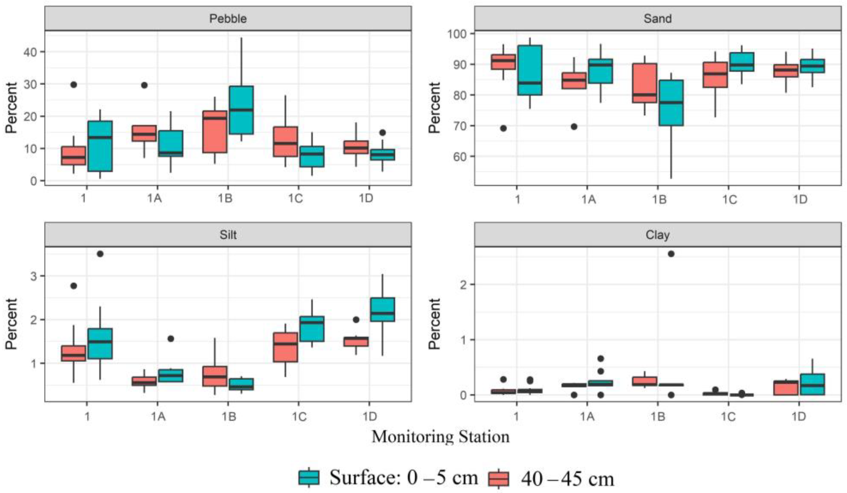
2.3. Soil Particle Fractionation

Soil particle fractionation was performed on all soil cores. Dried soil samples were reduced to finer grains first using a pestle and mortar [8,43,44]. Soil samples were then poured into sieve stacks to perform mechanical shaking for 15 min [8,43,44,45]. Three sieves of 4.76 mm, 0.25 mm, and 0.06 mm mesh sizes were used to separate pebble, coarse sand, and fine sand, respectively [46]. A base pan retained fine grains containing both silt and clay. Silt and clay soil partitions were separated using gravimetric filtration [8,43,44] with 2 µm Whatman filter papers. Filter papers were rinsed with deionized (DI) water using a volumetric flask, dried in the oven at 105 °C, and weighed. After preparing the filter papers, the fines were manually mixed with 100 mL of DI water to ensure complete particle mixing before being filtered using vacuum filtration. The silt fractions were left on the filter paper. After the filter paper was dried and weighed, the clay fraction was calculated by subtracting pebble, sand, and silt fractions from total weight fractions [8,43,44].

Statistical analyses like those described previously (Section 2.2) were performed to analyze the significant differences of soil particle fractions between monitoring sites and by depth. The soil texture for each core was estimated using the NRCS soil texture calculator [47].

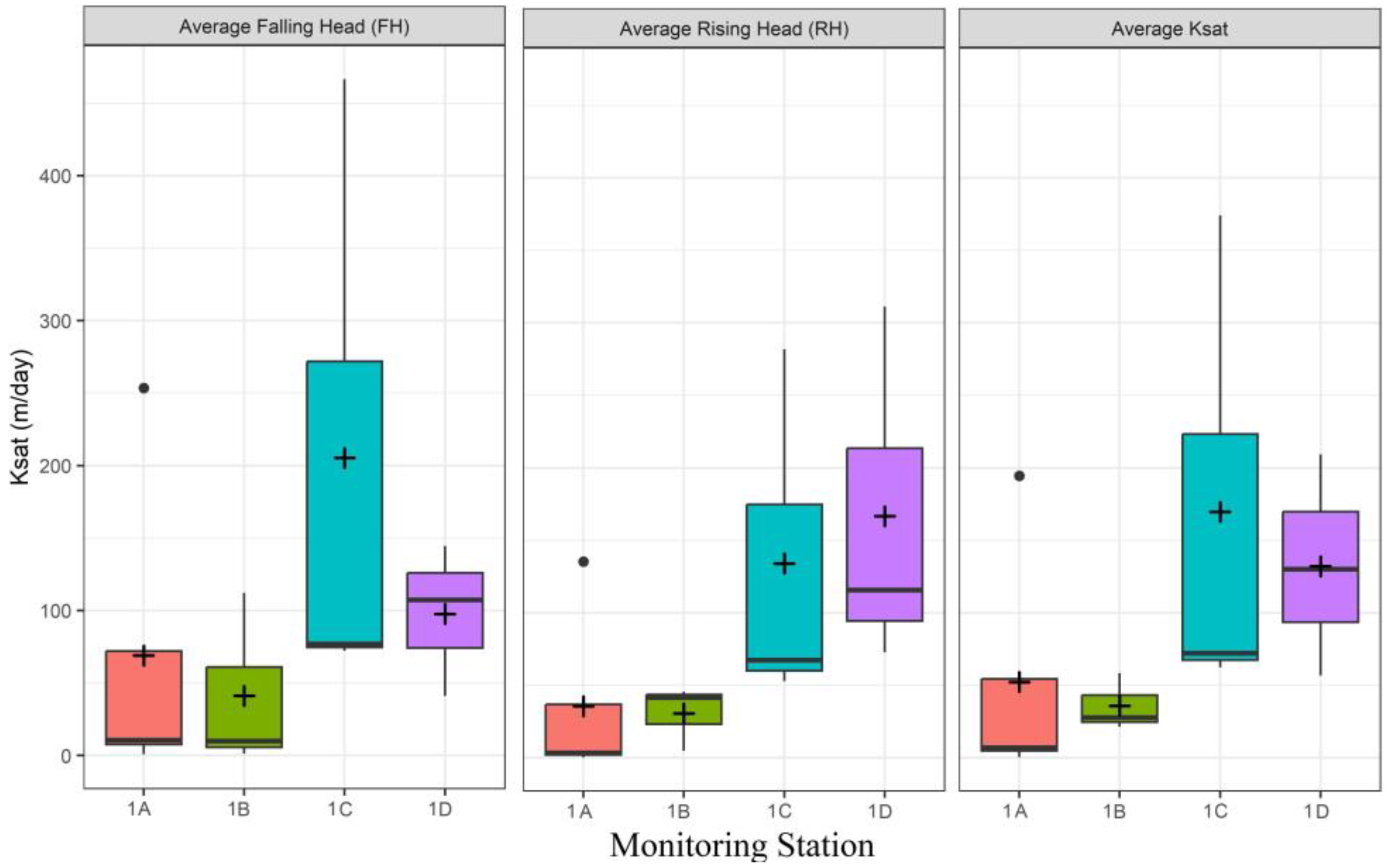
2.4. Observed Ksat Using Slug Tests

The study reach included 13 steel drive point piezometers with varying pipe lengths of 0.61–1.83 m, and total inner diameter, screened bottom segment, and drive point length of 0.03 m, 0.77 m, and 0.97 m, respectively. Rising head (RH) and falling head (FH) slug tests were conducted in each piezometer (n = 13) following the procedure outlined by [48] and [8]. Slug tests have shown to be effective in previous research for direct, in situ measurements of Ksat due to the low cost, simplicity, and faster measurement technique [8,48,49,50]. To conduct a slug tests, a Solinst 3001 Levelogger Edge M10 pressure transducer was placed in the bottom of the piezometer to record water level measurements at 0.125 s intervals. After 5–10 min, when the water table equilibrated to the volume of the sensor, a 170 cm³ copper slug was lowered into each piezometer. Water levels were equilibrated after approximately 15–30 min. Slug tests were repeated at least three times for each piezometer to replicate and validate the observed results statistically. Falling and rising head slug tests were averaged together using Equation (5) [51],

$$\mathrm{Ksat}=\frac{{\mathrm{r}}^2\ln (\frac{{\mathrm{L}}_{\mathrm{e}}}{\mathrm{R}})}{2{\mathrm{L}}_{\mathrm{e}}{\mathrm{t}}_{37}}$$

(5)

where r is the radius of the well casing (cm), R is the radius of the piezometer screen (cm), L_e is the length of the piezometer screen (cm), and t₃₇ (s) is the time it takes for the water level inside the piezometer to rise or fall 37% of the initial change during a slug test [44].

A paired sample T-test was performed to compare Ksat derived from RH and FH slug tests [40,41]. A one-way analysis of variance (ANOVA) was conducted to test for differences in Ksat between monitoring sites [8,40,41]. ANOVA was followed by Tukey–Kramer HSD to test for significant differences (CI = 95%, p < 0.05) in Ksat for each monitoring site pair in all possible combinations [8,40,41].

2.5. Selection of PTFs

Considering the use of various soil properties to estimate Ksat in previous studies [3,10,11,52], a Pearson correlation matrix and Principal Component Analysis (PCA) were conducted to identify the variation and correlation of the soil properties with Ksat. This analysis allowed for the selection of PTFs from the literature [17,18,19]. PCA generates an orthogonal uncorrelated axis, known as principal components (PCs), by transforming the original variables linearly [41]. PCs capture the maximum variation in the data set and are ordered based on their importance, with the first PC accounting for the most variance. The PCA algorithm derives the PCs by calculating the eigenvalue–eigenvector pairs of the correlation matrix of the original variables. The eigenvalue represents the variance explained by the principal components, while the eigenvector represents the orientation of the principal component axes relative to the original variables. The weight of each eigenvector is defined by loading, which explains how much each variable contributes to PCs [41]. Therefore, higher loading represents a higher relation between the variable and the corresponding PC.

2.6. Comparison of PTF Estimated Ksat with Observed Ksat

After performing the PCA and the Pearson correlation, five PTFs were chosen from the literature to estimate Ksat based on the soil property exhibiting a strong correlation with Ksat. To evaluate the performance of these PTFs, the PTF-estimated Ksat values were compared with the observed Ksat values using Mean Error (ME), Sum of Squared Error (SSE), and Root Mean Square Error (RMSE) following the methods of [8,12,17,22].

$$\mathrm{ME}={\sum }_{\mathrm{i}=1}^{\mathrm{n}}\frac{\mathrm{Ksat}\left(\mathrm{p}\right)\mathrm{i}-\mathrm{Ksat}\left(\mathrm{m}\right)\mathrm{i}}{\mathrm{n}}$$

(6)

$$\mathrm{SSE}=\sum _{\mathrm{i}=1}^{\mathrm{n}}{\left[\mathrm{Ksat}\left(\mathrm{p}\right)\mathrm{i}-\mathrm{Ksat}\left(\mathrm{m}\right)\mathrm{i}\right]}^2$$

(7)

$$\mathrm{RMSE}=\sqrt{\frac{\sum _{\mathrm{i}=1}^{\mathrm{N}}{\left[\mathrm{Ksat}\left(\mathrm{p}\right)\mathrm{i}-\mathrm{Ksat}\left(\mathrm{m}\right)\mathrm{i}\right]}^2}{\mathrm{n}}}$$

(8)

where Ksat(p)i is the predicted Ksat (m/d) from PTFs for each monitoring station of reach 12(i), Ksat(m)i is the measured average Ksat (m/d) from piezometer clusters of each monitoring station of reach 12$\left(\mathrm{i}\right)$, and n is the number of monitoring sites (n = 5).

3. Results and Discussions

3.1. Soil Characteristics

A total of one hundred and sixty soil cores were collected from the surface (0–5 cm) and at 40–45 cm depth from five monitoring sites (1, 1A, 1B, 1C, and 1D). The average soil bulk dry density (bdry) for the 45 cm depth was 1.34 g/cm³, 1.39 g/cm³, and 1.13 g/cm³ for sites 1, 1C, and 1D, respectively, and 1.25 g/m³ for both monitoring sites 1A and 1B. Across all monitoring sites, the porosity of the soil ranged from 0.47 to 0.57, with the lowest and highest porosity observed in sites 1 and 1D, respectively (Figure 2). 1D represented the highest (0.6) and 1B represented the lowest (0.37) volumetric water content (VWC) (Figure 2). Both 1C and 1D showed a high degree of saturation of 1.05, and 1, 1A, and 1B showed a degree of saturation of 0.95, 0.96, and 0.71, respectively.

The results of the two-way ANOVA indicated that depth significantly affected bdry, porosity, and VWC (p < 0.05). On average, for all the monitoring sites, the bdry at 40–45 cm depth was 39.42% higher than the surface bulk density (0–5 cm depth) (Figure 2). Conversely, porosity and VWC were 26% and 23% higher on the surface than 40–45 cm, respectively (Figure 2). The degree of saturation differed significantly among monitoring sites (p < 0.05), with 1B showing the lowest degree of saturation (0.71) for both depths. The average degree of saturation for all the monitoring sites was higher at 40–45 cm depth than at the surface, except for 1A (Figure 2).

3.2. Soil Texture Derived from Sieve Analyses

The results of the observed particle size fractionations are presented in

Table 1. Average soil textural percentages calculated from sieve analysis of soil samples from five study sites located in a tributary of West Run Watershed, Morgantown, WV. Soil samples were collected using a 4 × 4 grid at two depths (surface: 0–5 cm, and 40–45 cm). All texture results are percentage (%).

Texture	Site 1	Site 1A	Site 1B	Site 1C	Site 1D
Pebble	10.16	12.20	20.27	13.02	10.09
Medium Sand	66.18	67.41	57.16	60.38	57.09
Fine Sand	22.14	19.35	21.36	24.89	30.57
Total Sand	88.32	86.75	78.53	85.27	87.66
Silt	1.44	0.87	0.95	1.66	2.08
Clay	0.08	0.17	0.25	0.05	0.17

and Figure 3. For all the study sites, sand percentages were significantly higher than pebble, clay, and silt percentages (p < 0.05). Sand percentages ranged from 78.53% on station 1B to 88.32% on station 1 (Table 1). The sand percentages were followed by pebble percentages, which ranged from 10.16% to 20.27%. The study sites had minor silt (0.87–2.08%) and clay percentages (0.05–0.25%) (Table 1). On average, 60% of the sand was medium sand, while 40% was fine sand. No significant differences were observed among the reach study sites based on texture (p > 0.05), indicating that all the sites exhibited high sand and pebble with low silt and clay. Based on these results, the soil texture of the study reach was primarily sandy with loamy sand at station 1B.

Particle size fractions did not significantly vary by depth for all the study sites (p > 0.05) (Figure 3). The observed texture differed from the NRCS-predicted texture. NRCS predicted that the soils were Lobdell–Holly silt loam (50% silt, less than 20% clay) [34]. The differences in soil texture between the current study and the NRCS can be attributed to the sampling locations. In the current study, the soil samples were collected from the alluvial soil, which is expected to have a higher proportion of sand and pebble particles due to the sampling grids being closer to the reach [52]. In contrast, the NRCS soil sample was collected and analyzed on a larger regional scale [34], which is different than the current reach-focused study.

3.3. Observed Ksat Values from Slug Tests

Falling head (FH) and rising head (RH) slug tests were conducted, and the average Ksat was estimated at all piezometers in each cluster of the monitoring sites (n = 13). Overall, FH-generated Ksat values were more variable than RH Ksat values (

Table 2. Falling Head (FH) Ksat (m/d), Rising Head (RH) Ksat (m/d), and average Ksat (m/d) for the study reach, West Run Watershed, Morgantown, WV. The slug test was conducted at nested piezometers at monitoring sites 1A, 1B, 1C, and 1D. The average Ksat for the piezometer cluster of the monitoring site with the minimum and maximum Ksat values is shown parenthetically.

Monitoring Sites	FH Ksat	RH Ksat	Average Ksat
1A	68.92 (0.88, 253.52)	35.57 (0.02, 135.38)	52.25 (0.54, 194.45)
1B	41.12 (1.21, 112.08)	30.68 (4.80, 45.59)	35.90 (21.43, 58.44)
1C	205.25 (72.20, 466.54)	134.03 (52.80, 281.91)	169.64 (62.50, 374.22)
1D	97.62 (40.96, 144.44)	166.63 (72.82, 311.31)	132.12 (56.89, 209.38)

, Figure 4). FH Ksat values ranged from 0.88 to 466.54 m/d across all monitoring sites, while the RH Ksat values ranged from 0.02 to 311.31 m/d. This result was similar to the results from [8,53] in which the FH Ksats were generally higher than the RH Ksats owing to a higher flow resistance during the FH slug tests. Regardless, there was no significant difference between the Ksat values obtained from the FH and RH tests (p > 0.05) in the current study.

FH and RH Ksat values were averaged to get an overall average Ksat value for each observed piezometer (n = 13). This approach was taken so that average Ksat values from piezometer clusters (Table 2) were more representative and therefore more comparable to thr soil characteristics information generated for each site. A one-way ANOVA showed a significant difference in Ksat values among the monitoring sites (p < 0.05). Tukey’s post hoc multiple comparison tests revealed that monitoring sites 1C and 1D had significantly higher FH and RH Ksat values than station 1A (p < 0.05). Furthermore, in terms of average Ksat, station 1C exhibited the highest value (169.64 m/d), while station 1B had the lowest (35.90 m/d). Differences in Ksat values between monitoring sites represented inter-site Ksat heterogeneity for the reach. As Ksat is known to be influenced by soil structural and textural properties [19], higher Ksat values at site 1C could be attributed to a greater degree of saturation (Figure 2), along with higher silt content and lower clay content, compared with the other sites (Figure 3, Table 1). Higher saturation, increased silt, and decreased clay content can enhance pore space interconnectivity [38], resulting in greater water transport rates and higher Ksat values for site 1C. The water table depths for 1A–1D during slug tests were 28 cm, 57 cm, 59 cm and 47 cm, respectively. Except for site 1B, Ksat increased with depth (

Table A2. Water table depth (cm) during the slug tests and average Ksat (m/d) for the study reach, West Run Watershed, Morgantown, WV.

Monitoring Site	Water Table Depth (cm)	Ksat (m/d)
1A	28	52.25
1B	57	35.90
1C	59	169
1D	48	132

). It was observed that the degree of saturation was higher at 40–45 cm compared with the surface (Figure 2). Therefore, as soil depth increased, saturation levels rose, corresponding to increased Ksat estimates.

The reach-level average Ksat was 94 m/d, which was higher than the observed Ksat of NRCS (0.78 m/d) [35]. The differences between the NRCS-predicted Ksat and the observed slug test-generated Ksat values are attributed to differences in the field measurement techniques as NRCS generally measures Ksat using constant head well permeameters, double ring infiltrometers, and amoozemeters [36]. In addition, NRCS estimates Ksat using textural triangle diagrams based on soil texture and relative bulk density (low, medium, high) [36]. It is important to note that Ksat estimation is sensitive to additional factors such as sample size, flow geometry, and soil conditions [54], which may further contribute to the differences in Ksat observations between NRCS and the current study.

3.4. Modeling Ksat with PTFs

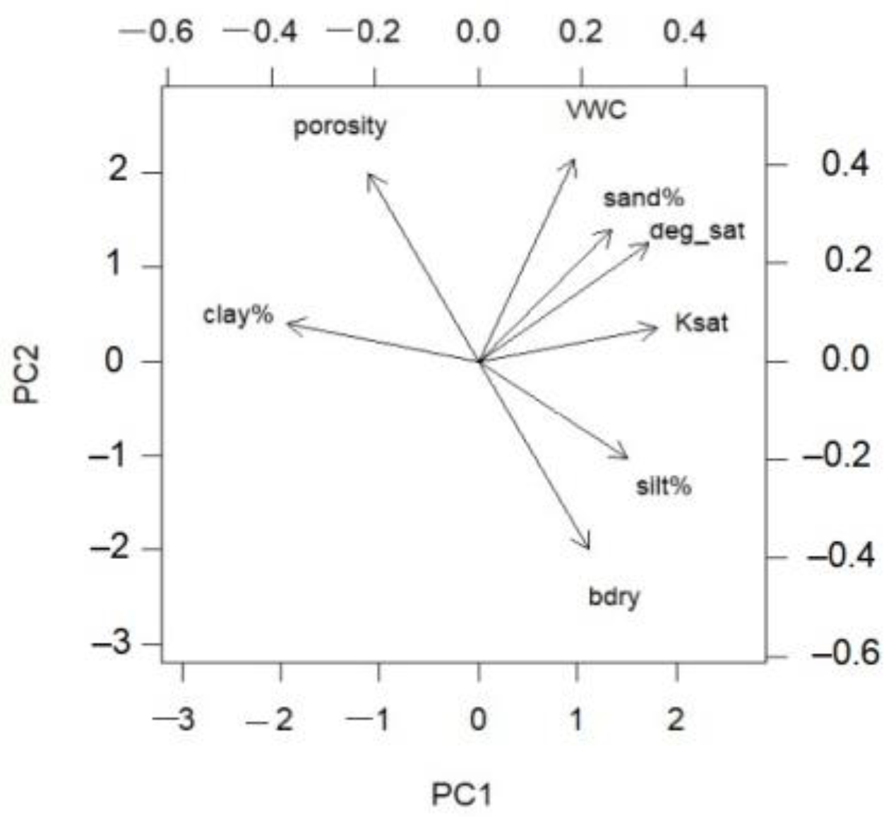
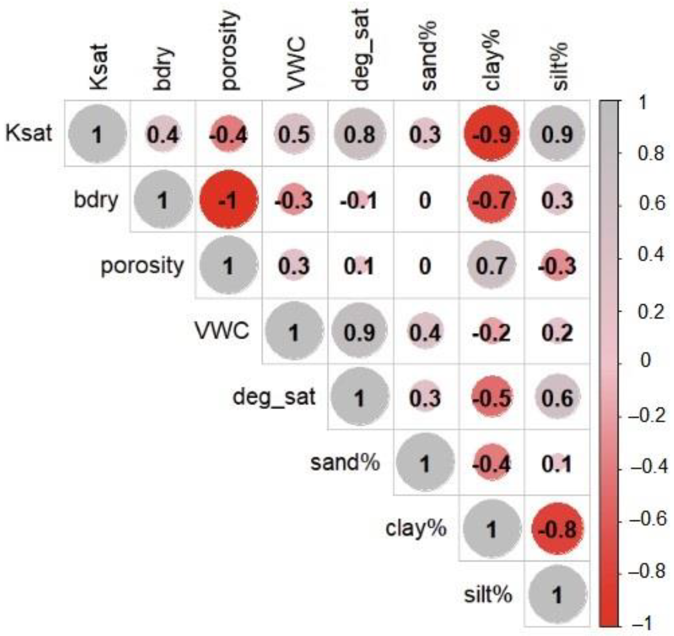
3.4.1. Principal Component Analysis (PCA) and Correlation between Soil Properties and Ksat

To facilitate the selection of appropriate PTFs from the literature for the current investigation, principal component analysis (PCA) and Pearson correlation were performed to understand the relation of observed soil properties with Ksat. To ensure consistency among variables with different measurement units or scales, the data were standardized by subtracting the mean of each variable and dividing it by its respective standard deviation [41]. Standardization ensured that the data were aligned on a common scale, with a mean of 0 and a standard deviation of 1 [41]. The PCA results indicated that the first two PCs (PC1 and PC2) cumulatively accounted for 89% of the variation in data, where PC1 and PC2 accounted for 53% and 36% of the variation, respectively (

Table 3. The eigenvalue, proportion of variance, and cumulative variance of each principal component (PC).

Principal Component	PC1	PC2	PC3	PC4	PC5
Eigenvalue	2.06	1.69	0.87	0.32	0
Proportion of variance	0.53	0.36	0.09	0.01	0
Cumulative Proportion	0.53	0.89	0.98	1	1

). Therefore, PC1 and PC2 were given the primary focus. A biplot was generated to illustrate the influence of each soil property on PC1 and PC2 (Figure 5). The biplot and loadings showed that Ksat, silt%, and the degree of saturation had a high positive correlation with PC1, and clay% had a strong negative correlation (

Table 4. Loading of each soil property for PC1 and PC2. Notes: Ksat: saturated hydraulic conductivity, Bdry: bulk dry density, VWC: volumetric water content, Sand%, Clay%, Silt%: sand, clay, and silt percentages. Loadings higher than 0.3 are in bold.

Soil Properties	PC1	PC2
Ksat	0.43	0.08
Bdry	0.27	−0.48
Porosity	−0.27	−0.48
VWC	0.23	0.51
Degree of saturation	0.41	0.30
Sand%	0.31	0.33
Clay%	−0.46	0.09
Silt%	0.36	−0.25

, Figure 5). Conversely, PC2 correlated highly with bdry, porosity, and VWC (Table 4, Figure 5). Therefore, PC1 and PC2 represented soil textural and structural properties. Ksat had a higher relationship with PC1 (loading: 0.43) than PC2 (loading: 0.08), illustrating a close alignment of Ksat with soil textural properties than soil structure (Table 4). Out of soil textural percentages, clay% demonstrated the highest negative correlation (−0.46), followed by the moderate correlation of silt% (0.36) and sand% (0.32) with PC1. Similarly, from the correlation matrix (Figure 6), it was shown that Ksat had a moderate correlation with bdry (0.4), porosity (−0.4), and VWC (0.5); a high correlation with clay% (−0.9) and silt% (0.9); and a very low correlation with sand% (0.3). Therefore, based on the PCA and the correlation analysis, five PTFs were selected to estimate Ksat as a function of soil texture, primarily clay percentages.

3.4.2. Selected PTFs

The following PTFs were chosen from the literature based on the preceding analysis.

The Puckett et al. Model

Puckett et al. [11] estimated Ksat as a function of clay percentage.

$$\mathrm{Ksat}=4.36 \times {10}^{-5} \times {\mathrm{e}}^{(-0.1975 \times \%\mathrm{clay})}$$

(9)

where Ksat is the predicted soil saturated hydraulic conductivity (m/s) and % clay represents the average dimensionless clay fraction.

The Smettem and Britsow Model

Smettem and Bristow [13] established a physio-empirical model based explicitly on clay content using several agricultural topsoil samples.

$$\mathrm{Ksat}=2500\times \mathrm{C} \times {\mathrm{h}}_{\mathrm{b}}^{-2}$$

(10)

h_b = 43.5/(−0.25 log% clay + 0.5)

(11)

where h_b is the bubbling pressure (mm), C is a constant equal to 144, %clay represents the average dimensionless fraction of clay, and Ksat is the predicted soil saturated hydraulic conductivity (mm/h) at each study site.

The Cosby et al. Model

Cosby et al. [14] proposed a model that used percentages of sand and clay contents to determine Ksat.

$$\mathrm{Ksat}=25.4+{10}^{\left(-0.6+0.012\mathrm{sand}-0.0064\mathrm{clay}\right)}$$

(12)

where Ksat is the predicted soil-saturated hydraulic conductivity (mm/h), and sand and clay represent the average dimensionless fraction of sand and clay, respectively.

The Dane and Puckett Model

Dane and Puckett [55] developed a non-linear regression model of 577 Ksat values collected from the Lower Coastal Plain of Alabama as a function of clay content.

$$\mathrm{Ksat}=8.44 \times {10}^{-5} \times {\mathrm{e}}^{-0.144\times \%\mathrm{clay}}$$

(13)

where Ksat is the predicted soil saturated hydraulic conductivity (m/s), and % clay represents the average dimensionless clay fraction.

The Campbell and Shiozawa Model

Campbell and Shiozawa [56] predicted Ksat from silt and clay percentages.

$$\mathrm{Ksat}=1.5 \times {10}^{-5}\exp \left(-7.0 \mathrm{silt}-16.7 \mathrm{clay}\right)$$

(14)

where Ksat is the predicted soil saturated hydraulic conductivity (m/s)z and silt and clay represent site average dimensionless fractions of silt and clay, respectively.

3.4.3. Ksat Estimates via Pedotransfer Functions (PTFs)

All the PTFs showed minor variations in the estimated Ksat values among each other (

Table 5. Ksat calculated from pedotransfer functions (PTFs) of the Puckett et al. [11] model, Smettem and Bristow [51] model, Cosby et al. [13] model, Dane and Puckett [55] model, and Campbell and Shiozawa [56] model. Note: All PTF Results are Ksat (m/d).

PTF Method	Site 1	Site 1A	Site 1B	Site 1C	Site 1D
Puckett et al.	3.77	3.77	3.77	3.78	3.77
Smettem and Bristow	7.49	6.49	6.04	8.02	6.50
Cosby et al.	0.62	0.62	0.62	0.62	0.62
Dane and Puckett	7.29	7.29	7.28	7.29	7.29
Campbell and Shiozawa	1.15	1.18	1.16	1.14	1.09

). From the reach level average, PTF estimated Ksat values ranged from a minimum value of 0.62 m/d using the Cosby et al. [14] model to a maximum value of 7.29 m/d generated using the Dane and Puckett Model [55] (Table 5). In contrast, the Ksat values obtained from the slug test ranged from 35.90 m/d to 169.64 m/d (Table 2), indicating more than one order of magnitude higher than those estimated by the PTFs. The observed discrepancies in the Ksat values between the slug test and the PTFs may be due to various factors. For example, the slug test may have averaged higher volumes, whereas the sieve analysis was limited by the volume of samples estimated using the soil core method [57]. Additionally, the discrepancies between the PTF-estimated Ksats and the observed Ksat in the current study reach can be attributed to differences in land use and topographic features between the study reach and the areas where the PTFs were originally developed. The selected PTFs were created using readily available soil textural data at a regional scale [11,14,56] and focused on specific land use areas. For example, Campbell and Shiozawa [56] developed their PTF using soil samples primarily from agricultural topsoil. However, the current study sites were located in a mixed land-use catchment, introducing potential discrepancies in the Ksat estimates. This finding aligned with the observations made by [22,25]. Duan et al. [22] noted that the PTF estimation accuracy was low in an area with healthy grass cover due to distinct soil characteristics and hydraulic properties specific to grass-covered soil. Similarly, Lim et al. [25] concluded that observed Ksat in forested soil samples were 10 to 10³ times larger than the estimated Ksat from PTFs, underscoring the limitations of using PTFs not specifically calibrated for forested soil to account for the influence of topography and vegetation.

3.5. Comparison of Observed Ksat Values and PTF Calculated Ksat Values

All the PTFs exhibited similar magnitudes of negative ME, indicating an underestimation of Ksat by PTFs. However, out of the five PTFs, the Smettem and Bristow [13] and Dane and Puckett [55] models performed better with ME ~ −90 m/d (

Table 6. Comparison between PTF-estimated Ksat values with slug test for each monitoring station using error, squared error, and reach-level ME, SSE, and RMSE calculated for the study reach, West Run Watershed (WRW), WV. Note: ME = mean error (m/d), SSE = Sum of squared error (m²/day²), RMSE = root mean square error (m/d).

Puckett et al. [11]			Smettem and Bristow [51]		Cosby et al. [13]		Dane and Puckett [55]		Campbell and Shiozawa [56]
Sites	Error	Squared Error	Error	Squared Error	Error	Squared Error	Error	Squared Error	Error	Squared Error
1	−93.71	8782.22	−89.99	8098.45	−96.86	9382.67	−90.19	8133.98	−96.32	9278.08
1A	−48.48	2350.72	−45.76	2093.61	−51.63	2666.11	−44.96	2021.37	−51.07	2607.63
1B	−32.13	1032.65	−29.86	891.90	−35.28	1245.00	−28.61	818.56	−34.74	1206.71
1C	−165.87	27,513.95	−161.62	26,120.41	−169.02	28,569.38	−162.35	26,357.00	−168.50	28,390.83
1D	−128.35	16,474.80	−125.61	15,779.00	−131.50	17,293.30	−124.83	15,582.43	−131.03	17,168.94
ME	−93.71		−90.57		−96.86		−90.19		−96.33
SSE	56,154.34		52,983.38		59,156.47		52,913.34		58,652.2
RMSE	105.98		102.94		108.77		102.87		108.31

). The Campbell and Shiozawa [56] and Cosby et al. [14] models, which estimated Ksat as a function of two parameters, had an ME of −96.33 m/d and −96.86 m/d, respectively. This result differed from [8], where PTFs with two parameters provided increased estimation accuracy of Ksat relative to one parameter PTFs. Campbell–Shizowa [56] and Cosby et al. [14] models, respectively, used silt% and sand% with clay%. However, all the other PTFs used only clay percentages to predict Ksat. More soil properties exhibit greater spatial variability in Ksat due to topographic position, inter-site heterogeneity, and land-use differences, which may decrease the predictive accuracy of the PTF models [22]. Therefore, in the current work, the simplified single-parameter PTF, the Dane and Puckett [55] model, and the Smettem and Bristow [13] model provided greater Ksat estimation accuracy.

There were no significant differences between the RMSE of the five PTFs. However, the Dane and Puckett model [55] exhibited greater predictive accuracy with an RMSE of 102.87 m/d, while the Cosby et al. [14] model had lower prediction accuracy with an RMSE of 108.77 m/d. Similarly, SSE ranged from 52,913.34 m²/day² to 59,156.47 m²/day², with the Dane and Puckett [55] model showing the lowest SSE and the Cosby et al. model showing the highest SSE. Monitoring site 1B had the lowest error; among all the sites, it had the highest clay percentages and the lowest total sand (Table 4). Overall, the PTFs that calculated Ksat as a function of clay content exhibited the best results. These results may be attributable to the high correlation between Ksat and clay percentage (−0.9), and the low correlation between Ksat and sand percentage (0.3), as shown in Figure 6. Additionally, PCA analysis suggested a strong relationship between Ksat and clay content with PC1 and each other (Figure 5, Table 4). Therefore, performing PCA and analyzing the correlation between soil textural and structural properties with Ksat proved helpful in selecting PTFs.

Overall, the predictive accuracy of all five PTFs was limited, which could be attributed to the mixed land-use practices of the current study area. Ksat is generally reported to vary under different land-management practices [58,59,60]. For example, in forests and grasslands, Ksat is generally higher due to the presence of organic matter, the root growth of trees, and burrowing mammals contributing to higher soil porosity and infiltration rates [38,58,59,60]. Furthermore, forest soil Ksats are influenced by a diverse range of plants, trees, and decomposed leaves, setting them apart from the characteristics of grassland and bareland soils [25]. In contrast, anthropogenic activities, such as road construction and buildings, increase impervious surfaces, decreasing pore space and infiltration rates and affecting Ksat [38]. The impact of mixed land use on Ksat is complex, with the contribution of forest, agriculture, and impervious areas influencing soil hydraulic properties differently. The heterogeneity of Ksat in mixed land-use watersheds cannot be fully captured by using PTFs developed for a single land use or soil texture [10,13,14]. Therefore, it is needed to adjust the existing PTFs by thoroughly examining soil characteristics and gathering Ksat data from large scale mixed land-use catchments. This approach is crucial to achieving precise estimations of Ksat values while considering the diverse impact of mixed land use on Ksat.

3.6. Limitations and Future Direction

The current study had certain limitations that should be acknowledged. First, the PTFs utilized in this research were not developed or adjusted for riparian wetlands of a mixed land-use watershed. This discrepancy in land-use practices might have introduced a degree of uncertainty in predicting Ksat [22,25]. Additionally, the sample size in the study was limited due to various study limitations. Furthermore, there is a lack of readily available reach-scale soil characteristics and a Ksat database, which affected the availability of comprehensive data for analysis. With these potential limitations in mind, the current study showed that all PTFs underestimated Ksat values relative to the observed Ksat values. This result suggests that existing PTFs must be adjusted, or new PTFs must be developed, that can accurately estimate Ksat in complex mixed land-use areas. To achieve this, new PTFs should be calibrated using large-scale soil structural and textural properties and validated with observed Ksat values. Regression analysis using PCs derived from principal component analysis (PCA) can facilitate the development of future PTFs. For example, a new PTF was developed by relating the log(Ksat) with PC1 through linear regression analysis (Equation (15)), as PC1 estimated 53% of the data variance.

$$\log \left(\mathrm{Ksat}\right)=4.43+0.27 \mathrm{PC}1$$

(15)

The regression analysis was conducted following the methods described by [18]. Additional information is provided in Appendix A. The new model improved the prediction accuracy of Ksat, with the ME, SSE, and RMSE of −4.6 m/d, 4547 m²/d², and 30.16 m/d, respectively, outperforming the five existing PTFs. However, additional soil structural and textural properties, such as field capacity, soil organic matter, wilting point, carbonate content, and sodium adsorption ratio, are closely related to Ksat and their inclusion may improve the outcomes of the development of new PTFs [19,61]. For example, riparian wetland soils often include high organic matter [62] and the inclusion of organic matter content might increase the predictive accuracy of PTFs [19,61,63]. While the assessment of organic matter was beyond the scope of the current research, this provides an impetus for future investigations. Furthermore, the dataset used for model development and validation was small, consisting of only five observations, which limits the ability to assess the robustness of the newly developed PTF function. Therefore, future studies need to incorporate more soil properties and validate the developed PTF by collecting large scale soil samples from riparian wetlands of similar land use.

4. Conclusions

The predictive accuracy of pedotransfer functions (PTFs) needs to be analyzed to accurately estimate Ksat in seasonal riparian wetlands of the mixed land-use West Run Watershed (WRW) located in northeastern Morgantown, West Virginia (WV). To validate the PTFs, observed Ksat values were collected through the rising head (RH) and falling head (FH) slug tests conducted at the nested piezometers of four monitoring sites on the study reach. The average Ksat ranged from the maximum value of 169.64 m/d at site 1C to the minimum value of 35.90 m/d at site 1B. The selection of PTFs was based on the correlation between soil properties and Ksat, determined using Pearson correlation and Principal Component Analysis (PCA). Soil cores from two depths (surface: 0–5 cm, and 40–45 cm) were analyzed to assess soil structural and textural properties. The results revealed a significant increase in average soil bulk dry density (bdry) with depth (p < 0.05), ranging from 1.39 to 1.13 g/cm³, while porosity and volumetric water content (VWC) decreased (p < 0.05). The degree of saturation varied, with site 1C having the highest value (1.05) and station 1B the lowest (0.71). Sandy soil texture predominated within the study reach. PCA indicated that the first and second principal components (PC1 and PC2) cumulatively explained 89% of the variation in data with PC1 and PC2, respectively, explaining 53% and 36% of the variation. Soil textural properties were correlated with the PC1, while soil structural properties were correlated with PC2. Ksat had a higher relationship with PC1 than PC2. Additionally, the Pearson correlation analysis indicated that Ksat had a strong negative correlation with clay% and a strong positive correlation with silt%, while its correlation with sand% was very low. Based on this understanding, five PTFs were selected, primarily using clay% to calculate Ksat. Comparing the PTF-estimated Ksat values with the observed data, the Dane and Puckett model demonstrated the highest accuracy (ME = −90.19 m/d, RMSE = 102.87 m/d), while the Cosby et al. model exhibited the lowest accuracy (ME = −96.86 m/d, RMSE = 108.77). PTFs incorporating clay% outperformed those using silt% or sand% in combination with clay%, highlighting the importance of understanding the relationship between soil properties and Ksat for selecting suitable PTFs. However, the five PTFs tested had limited success in estimating Ksat, possibly due to the mixed land-use characteristics of the study area. Therefore, there is a need to calibrate existing PTFs with local soil properties or develop new ones, which can be validated with Ksat data collected from large scale mixed land-use catchments. Despite the study’s limitations, it represents one of the pioneering efforts to examine PTFs in the riparian wetlands of mixed land-use catchments. This research provides valuable insights for land managers in developing effective water management strategies by enhancing the understanding of water flow dynamics through Ksat assessment. Furthermore, the findings of this study can contribute to improving the accuracy of model predicted Ksat values and can serve as a benchmark for future PTF development and validation in similar landscapes.

References

1. Darcy, H. The Public Fountains of the City of Dijon; Dalmont: Paris, France, 1856. [Google Scholar]
2. Hwang, H.T.; Jeen, S.W.; Suleiman, A.A.; Lee, K.K. Comparison of Saturated Hydraulic Conductivity Estimated by Three Different Methods. Water 2017, 9, 942. [Google Scholar] [CrossRef] [Green Version]
3. Jabro, J.D. Estimation of Saturated Hydraulic Conductivity of Soils from Particle Size Distribution and Bulk Density Distribution and Bulk Density Data. Trans. Am. Soc. Agric. Eng. 1992, 35, 557–560. [Google Scholar] [CrossRef]
4. Monreal, T.E.; Julia, M.F.; Jime, C.; Garcı, E.; Sa, A. Constructing a Saturated Hydraulic Conductivity Map of Spain Using Pedotransfer Functions and Spatial Prediction. Geoderma 2004, 123, 257–277. [Google Scholar] [CrossRef]
5. Montzka, C.; Herbst, M.; Weihermüller, L.; Verhoef, A.; Vereecken, H. A Global Data Set of Soil Hydraulic Properties and Sub-Grid Variability of Soil Water Retention and Hydraulic Conductivity Curves. Earth Syst. Sci. Data 2017, 9, 529–543. [Google Scholar] [CrossRef] [Green Version]
6. Zhang, Y.; Schaap, M.G. Estimation of Saturated Hydraulic Conductivity with Pedotransfer Functions: A Review. J. Hydrol. 2019, 575, 1011–1030. [Google Scholar] [CrossRef]
7. Cheong, J.Y.; Hamm, S.Y.; Kim, H.S.; Ko, E.J.; Yang, K.; Lee, J.H. Estimating Hydraulic Conductivity Using Grain-Size Analyses, Aquifer Tests, and Numerical Modeling in a Riverside Alluvial System in South Korea. Hydrogeol. J. 2008, 16, 1129–1143. [Google Scholar] [CrossRef]
8. Gootman, K.; Kellner, E.; Hubbart, J. A Comparison and Validation of Saturated Hydraulic Conductivity Models. Water 2020, 12, 2040. [Google Scholar] [CrossRef]
9. Vienken, T.; Dietrich, P. Field Evaluation of Methods for Determining Hydraulic Conductivity from Grain Size Data. J. Hydrol. 2011, 400, 58–71. [Google Scholar] [CrossRef]
10. Saxton, K.E.; Rawls, W.J.; Romberger, J.S.; Papendick, R.I. Estimating Generalized Soil-Water Characteristics from Texture. Soil Sci. Soc. Am. J. 1986, 50, 1031–1036. [Google Scholar] [CrossRef]
11. Puckett, W.E.; Dane, J.H.; Hajek, B.F. Physical and Mineralogical Data to Determine Soil Hydraulic Properties. Soil Sci. Soc. Am. J. 1985, 49, 831–836. [Google Scholar] [CrossRef]
12. Van Looy, K.; Bouma, J.; Herbst, M.; Koestel, J.; Minasny, B.; Mishra, U.; Montzka, C.; Nemes, A.; Pachepsky, Y.A.; Padarian, J.; et al. Pedotransfer Functions in Earth System Science: Challenges and Perspectives. Rev. Geophys. 2017, 55, 1199–1256. [Google Scholar] [CrossRef] [Green Version]
13. Smettem, K.R.J.; Bristow, K.L. Obtaining Soil Hydraulic Properties for Water Balance and Leaching Models from Survey Data. 2. Hydraulic Conductivity. Aust. J. Agric. Res. 1999, 50, 1259. [Google Scholar] [CrossRef]
14. Cosby, B.J.; Hornberger, G.M.; Clapp, R.B.; Ginn, T.R. A Statistical Exploration of the Relationships of Soil Moisture Characteristics to the Physical Properties of Soils. Water Resour. Res. 1984, 20, 682–690. [Google Scholar] [CrossRef] [Green Version]
15. Chapuis, R.P. Predicting the Saturated Hydraulic Conductivity of Sand and Gravel Using Effective Diameter and Void Ratio. Can. Geotech. J. 2004, 41, 787–795. [Google Scholar] [CrossRef]
16. Urumović, K. The Referential Grain Size and Effective Porosity in the Kozeny-Carman Model. Hydrol. Earth Syst. Sci. 2016, 20, 1669–1680. [Google Scholar] [CrossRef] [Green Version]
17. Zuo, Y.; He, K. Evaluation and Development of Pedo-Transfer Functions for Predicting Soil Saturated Hydraulic Conductivity in the Alpine Frigid Hilly Region of Qinghai Province. Agronomy 2021, 11, 1581. [Google Scholar] [CrossRef]
18. Duffera, M.; White, J.G.; Weisz, R. Spatial Variability of Southeastern U.S. Coastal Plain Soil Physical Properties: Implications for Site-Specific Management. Geoderma 2007, 137, 327–339. [Google Scholar] [CrossRef]
19. Gamie, R.; De Smedt, F. Experimental and Statistical Study of Saturated Hydraulic Conductivity and Relations with Other Soil Properties of a Desert Soil: Hydraulic Conductivity of a Desert Soil. Eur. J. Soil Sci. 2018, 69, 256–264. [Google Scholar] [CrossRef] [Green Version]
20. Wang, Y.; Shao, M.; Liu, Z.; Horton, R. Regional-Scale Variation and Distribution Patterns of Soil Saturated Hydraulic Conductivities in Surface and Subsurface Layers in the Loessial Soils of China. J. Hydrol. 2013, 487, 13–23. [Google Scholar] [CrossRef]
21. Xu, C.; Xu, X.; Liu, M.; Liu, W.; Yang, J.; Luo, W.; Zhang, R.; Kiely, G. Enhancing Pedotransfer Functions (PTFs) Using Soil Spectral Reflectance Data for Estimating Saturated Hydraulic Conductivity in Southwestern China. CATENA 2017, 158, 350–356. [Google Scholar] [CrossRef]
22. Duan, R.; Fedler, C.B.; Borrelli, J. Comparison of Methods to Estimate Saturated Hydraulic Conductivity in Texas Soils with Grass. J. Irrig. Drain. Eng. 2012, 138, 322–327. [Google Scholar] [CrossRef]
23. Minasny, B.; McBratney, A.B. Evaluation and Development of Hydraulic Conductivity Pedotransfer Functions for Australian Soil. Aust. J. Soil Res. 2000, 38, 905–926. [Google Scholar] [CrossRef]
24. Pachepsky, Y.A.; Rawls, W.J.; Timlin, D.J. The Current Status of Pedotransfer Functions: Their Accuracy, Reliability, and Utility in Field- and Regional-Scale Modeling. In Geophysical Monograph Series; Corwin, L., Loague, K., Ellsworth, R., Eds.; American Geophysical Union: Washington, DC, USA, 1999; Volume 108, pp. 223–234. ISBN 978-0-87590-091-9. [Google Scholar]
25. Lim, H.; Yang, H.; Chun, K.W.; Choi, H.T. Development of Pedo-Transfer Functions for the Saturated Hydraulic Conductivity of Forest Soil in South Korea Considering Forest Stand and Site Characteristics. Water 2020, 12, 2217. [Google Scholar] [CrossRef]
26. Petryk, A.; Kruk, E.; Ryczek, M.; Lackóová, L. Comparison of Pedotransfer Functions for Determination of Saturated Hydraulic Conductivity for Highly Eroded Loess Soil. Land 2023, 12, 610. [Google Scholar] [CrossRef]
27. Huisman, J.A.; Breuer, L.; Frede, H.-G. Sensitivity of Simulated Hydrological Fluxes towards Changes in Soil Properties in Response to Land Use Change. Phys. Chem. Earth 2004, 29, 749–758. [Google Scholar] [CrossRef]
28. Spruill, C.A.; Workman, S.R.; Taraba, J.L. Simulation of Daily and Monthly Stream Discharge from Small Watersheds Using SWAT Model. Trans. ASAE 2000, 43, 1431–1439. [Google Scholar] [CrossRef]
29. Abesh, B.F.; Liu, G.; Vázquez-Ortega, A.; Gomezdelcampo, E.; Roberts, S. Cyanotoxin transport from surface water to groundwater: Simulation scenarios for Lake Erie. J. Great Lakes Res. 2022, 48, 695–706. [Google Scholar] [CrossRef]
30. Mohajerani, H.; Teschemacher, S.; Casper, M.C. A Comparative Investigation of Various Pedotransfer Functions and Their Impact on Hydrological Simulations. Water 2021, 13, 1401. [Google Scholar] [CrossRef]
31. Weihermüller, L.; Lehmann, P.; Herbst, M.; Rahmati, M.; Verhoef, A.; Or, D.; Jacques, D.; Vereecken, H. Choice of Pedotransfer Functions Matters When Simulating Soil Water Balance Fluxes. J. Adv. Model. Earth Syst. 2021, 13, e2020MS002404. [Google Scholar] [CrossRef]
32. Horne, J.P.; Hubbart, J.A. A Spatially Distributed Investigation of Stream Water Temperature in a Contemporary Mixed-Land-Use Watershed. Water 2020, 12, 1756. [Google Scholar] [CrossRef]
33. Petersen, F.; Hubbart, J.A. Advancing Understanding of Land Use and Physicochemical Impacts on Fecal Contamination in Mixed-Land-Use Watersheds. Water 2020, 12, 1094. [Google Scholar] [CrossRef] [Green Version]
34. Wright, E.L.; Charles, H.D.; Sponaugle, K.; Cole, C.; Ammons, J.T.; Gorman, J.; Childs, F.D. Soil Conservation Service Soil Survey of Marion and Monongalia Counties, West Virginia; U.S. Department of Agriculture, Natural Resources Conservation Service: Washington, DC, USA, 1982.
35. Soil Survey Staff, Natural Resources Conservation Service, United States Department of Agriculture. Soil Survey Geographic (SSURGO) Database for [Monongalia, WV]. Available online: https://www.nrcs.usda.gov/resources/data-and-reports/soil-survey-geographic-database-ssurgo (accessed on 28 January 2023).
36. Schoeneberger, P.J.; Wysocki, D.A.; Benham, E.C.; Stuff, S.S. Field Book for Describing and Sampling Soils, Version 3.0; Natural Resources Conservation Service NRCS, National Soil Survey Center: Lincoln, NE, USA, 2012. Available online: https://www.nrcs.usda.gov/sites/default/files/2022-09/field-book.pdf (accessed on 24 June 2023).
37. Blake, G.R. Bulk Density. In Methods of Soil Analysis: Part 1-Physical and Mineralogical Properties, Including Statistics of Measurement and Sampling; Black, C.A., Evans, D.D., White, J.L., Ensminger, L.E., Clark, F.E., Dinauer, R.C., Eds.; American Society of Agronomy: Madison, WI, USA, 1965; pp. 374–390. [Google Scholar]
38. Dingman, S.L. Physical Hydrology; Waveland Press: Long Grove, IL, USA, 2015. [Google Scholar]
39. Vomocil, J.A. Porosity. In Methods of Soil Analysis: Part 1-Physical and Mineralogical Properties, Including Statistics of Measurement and Sampling; Black, C.A., Evans, D.D., White, J.L., Ensminger, L.E., Clark, F.E., Dinauer, R.C., Black, C.A., Eds.; American Society of Agronomy: Madison, WI, USA, 1965; pp. 299–314. ISBN 978-0-89118-203-0. [Google Scholar]
40. Crawley, M.J. Statistics: An Introduction Using R; John Wiley & Sons: Chichester, UK, 2005; ISBN 0-470-02298-1. [Google Scholar]
41. Davis, J.C. Statistics and Data Analysis in Geology, 3rd ed.; J. Wiley: New York, NY, USA, 2002; ISBN 0-471-17275-8. [Google Scholar]
42. R Core Team. R: A Language and Environment for Statistical Computing; R Foundation for Statistical Computing: Vienna, Austria, 2022; Available online: https://www.r-project.org/ (accessed on 1 January 2023).
43. Day, P.R. Particle Fractionation and Particle-Size Analysis. In Methods of Soil Analysis: Part 1 Physical and Mineralogical Properties, Including Statistics of Measurement and Sampling; Black, C.A., Evans, D.D., White, J.L., Ensminger, L.E., Clark, F.E., Dinauer, R.C., Eds.; American Society of Agronomy: Madison, WI, USA, 1965; pp. 545–567. [Google Scholar]
44. Gee, G.W.; OR, D. Particle-Size Analysis. In Methods of Soil Analysis. Part 4. Phyiscal Methods; Dane, J.H., Topp, G.C., Eds.; ACSESS: Madison, WI, USA, 2002; pp. 255–293. ISBN 978-0-89118-893-3. [Google Scholar]
45. McCave, I.N.; Syvitski, J.P.M. Principles and Methods of Geological Particle Size Analysis. In Principles, Methods and Application of Particle Size Analysis; Syvitski, J.P.M., Ed.; Cambridge University Press: Cambridge, UK, 1991; pp. 3–21. ISBN 978-0-521-36472-0. [Google Scholar]
46. Wentworth, C.K. A Scale of Grade and Class Terms for Clastic Sediments. J. Geol. 1922, 30, 377–392. [Google Scholar] [CrossRef]
47. Natural Resources Conservation Service (NRCS) Soil Texture Calculator. Available online: https://www.nrcs.usda.gov/resources/education-and-teaching-materials/soil-texture-calculator (accessed on 28 January 2023).
48. Butler, J.J. The Design, Performance, and Analysis of Slug Tests, 2nd ed.; CRC Press: Boca Raton, FL, USA, 2019; ISBN 978-0-367-81550-9. [Google Scholar]
49. Bouwer, H.; Rice, R.C. A Slug Test for Determining Hydraulic Conductivity of Unconfined Aquifers with Completely or Partially Penetrating Wells. Water Resour. Res. 1976, 12, 423–428. [Google Scholar] [CrossRef] [Green Version]
50. Noll, M.L.; Chu, A.; Capurso, W.D. Slug-Test Analysis of Selected Wells at an Earthen Dam Site in Southern Westchester County, New York; Open-File Report; U.S. Deaprtment of Interior, U.S. Geological Survey: Reston, VA, USA, 2019.
51. Hvorslev, M.J. Time Lag and Soil Permeability in Ground-Water Observations; Bulletion N0. 36; Waterways Experiment Station, Corps of Engineers, US Army: Vicksburg, MS, USA, 1951; pp. 1–55.
52. Nguyen, P.M.; Van Le, K.; Botula, Y.-D.; Cornelis, W.M. Evaluation of Soil Water Retention Pedotransfer Functions for Vietnamese Mekong Delta Soils. Agric. Water Manag. 2015, 158, 126–138. [Google Scholar] [CrossRef]
53. Malusis, M.A.; Barlow, L.C. Comparison of Laboratory and Field Measurements of Backfill Hydraulic Conductivity for a Large-Scale Soil-Bentonite Cutoff Wall. J. Geotech. Geoenviron. Eng. 2020, 146, 04020070. [Google Scholar] [CrossRef]
54. Reynolds, W.D.; Bowman, B.T.; Brunke, R.R.; Drury, C.F.; Tan, C.S. Comparison of Tension Infiltrometer, Pressure Infiltrometer, and Soil Core Estimates of Saturated Hydraulic Conductivity. Soil Sci. Soc. Am. J. 2000, 64, 478–484. [Google Scholar] [CrossRef]
55. Dane, J.H.; Puckett, W. Field Soil Hydraulic Properties Based on Physical and Mineralogical Information. In Proceedings of the International Workshop on Indirect Methods for Estimating the Hydraulic Properties of Unsaturated Soils, Riverside, CA, USA, 11–13 October 1989; van Genuchten, M.T., Leij, F.J., Eds.; U.S. Salinity Laboratory: Riverside, CA, USA, 1994; Volume 46, pp. 389–403. [Google Scholar]
56. Campbell, G.S.; Shiozawa, S. Prediction of Hydraulic Properties of Soils Using Particle Size Distribution and Bulk Density Data. In Proceedings of the International Workshop on Indirect Methods for Estimating the Hydraulic Properties of Unsaturated Soils, Riverside, CA, USA, 11–13 October 1989; van Genuchten, M.T., Leij, F.J., Eds.; U.S. Salinity Laboratory: Riverside, CA, USA, 1994. [Google Scholar]
57. Dietze, M.; Dietrich, P. Evaluation of Vertical Variations in Hydraulic Conductivity in Unconsolidated Sediments. Ground Water 2012, 50, 450–456. [Google Scholar] [CrossRef] [PubMed]
58. Deb, S.K.; Shukla, M.K. Variability of Hydraulic Conductivity due to Multiple Factors. Am. J. Environ. Sci. 2012, 8, 489–502. [Google Scholar] [CrossRef] [Green Version]
59. Kurnianto, S.; Selker, J.; Boone Kauffman, J.; Murdiyarso, D.; Peterson, J.T. The Influence of Land-Cover Changes on the Variability of Saturated Hydraulic Conductivity in Tropical Peatlands. Mitig. Adapt. Strateg. Glob. Chang. 2019, 24, 535–555. [Google Scholar] [CrossRef]
60. Zhou, X.; Lin, H.S.; White, E.A. Surface Soil Hydraulic Properties in Four Soil Series under Different Land Uses and Their Temporal Changes. CATENA 2008, 73, 180–188. [Google Scholar] [CrossRef]
61. Wang, M.; Liu, H.; Lennartz, B. Small-Scale Spatial Variability of Hydro-Physical Properties of Natural and Degraded Peat Soils. Geoderma 2021, 399, 115123. [Google Scholar] [CrossRef]
62. Oelbermann, M.; Raimbault, B.A. Riparian Land-Use and Rehabilitation: Impact on Organic Matter Input and Soil Respiration. Environ. Manag. 2015, 55, 496–507. [Google Scholar] [CrossRef] [PubMed]
63. Ganiyu, S.A. Evaluation of Soil Hydraulic Properties under Different Non-Agricultural Land Use Patterns in a Basement Complex Area Using Multivariate Statistical Analysis. Environ. Monit. Assess. 2018, 190, 595. [Google Scholar] [CrossRef] [PubMed]
Figure 1. Project study reach within the larger West Run Watershed with five stream stage monitoring sites (1, 1A, 1B, 1C, and 1D) including thirteen nested piezometers in West Run Watershed (WRW), West Virginia (WV), USA.
Water 15 02711 g001
Figure 2. Box and whisker plots of soil characteristics, including dry bulk density (bdry), porosity, volumetric water content (VWC), and degree of saturation for the study reach, West Run Watershed (WRW), West Virginia (WV), USA. The soil cores were collected from two depths; surface: 0–5 cm, and 40–45 cm. The black filled circle represents potential outliers.
Water 15 02711 g002
Figure 3. Box and whisker plot of soil textural percentages (pebble, sand, silt, and clay) from two depths (surface: 0–5 cm, and 40–45 cm) and five monitoring sites (1, 1A, 1B, 1C, 1D) of the study reach located in West Run Watershed (WRW), Morgantown, WV. The black filled circle represents potential outliers.
Water 15 02711 g003
Figure 4. Box and whisker plots of falling head (FH) Ksat (m/d), rising head (RH) Ksat (m/d), and average Ksat (m/d) for the study reach, West Run Watershed (WRW), Morgantown, WV. Slug tests were conducted at nested piezometers at monitoring sites 1A, 1B, 1C, and 1D. “+” = average Ksat values from piezometer clusters for each monitoring site. The black filled circle represents potential outliers.
Water 15 02711 g004
Figure 5. Biplot represents the relation between soil properties and PC1 and PC2. Ksat: saturated hydraulic conductivity, bdry: dry bulk density, VWC: volumetric water content, deg_sat: degree of saturation, Sand%, Clay%, Silt%: sand, clay, and silt percentages.
Water 15 02711 g005
Figure 6. Pearson correlation coefficient between soil properties where big and small circles represent high and low correlation, respectively. Red circles represent a highly negative correlation, and grey circles represent a highly positive correlation. Ksat: saturated hydraulic conductivity, bdry: bulk dry density, VWC: volumetric water content, deg_sat: degree of saturation, Sand%, Clay%, Silt%: sand, clay, and silt percentages.
Water 15 02711 g006