Article

Salinity Modeling Using Deep Learning with Data Augmentation and Transfer Learning

1
Department of Electrical and Computer Engineering, University of California, Davis, CA 95616, USA
2
California Department of Water Resources, 1516 9th Street, Sacramento, CA 95814, USA
3
Department of Computer Science, University of California, Davis, CA 95616, USA
4
Department of Mathematics, University of California, Davis, CA 95616, USA
*
Authors to whom correspondence should be addressed.
Water 2023, 15(13), 2482; https://doi.org/10.3390/w15132482
Submission received: 2 June 2023 / Revised: 1 July 2023 / Accepted: 4 July 2023 / Published: 6 July 2023
(This article belongs to the Special Issue Water Quality Modeling and Monitoring II)

Abstract

:
Salinity management in estuarine systems is crucial for developing effective water-management strategies to maintain compliance and understand the impact of salt intrusion on water quality and availability. Understanding the temporal and spatial variations of salinity is a keystone of salinity-management practices. Process-based numerical models have been traditionally used to estimate the variations in salinity in estuarine environments. Advances in data-driven models (e.g., deep learning models) make them effective and efficient alternatives to process-based models. However, a discernible research gap exists in applying these advanced techniques to salinity modeling. The current study seeks to address this gap by exploring the innovative use of deep learning with data augmentation and transfer learning in salinity modeling, exemplified at 23 key salinity locations in the Sacramento–San Joaquin Delta which is the hub of the water-supply system of California. Historical, simulated (via a hydrodynamics and water quality model), and perturbed (to create a range of hydroclimatic and operational scenarios for data-augmentation purposes) flow, and salinity data are used to train a baseline multi-layer perceptron (MLP) and a deep learning Residual Long-Short-Term Memory (Res-LSTM) network. Four other deep learning models including LSTM, Residual Network (ResNet), Gated Recurrent Unit (GRU), and Residual GRU (Res-GRU) are also examined. Results indicate that models pre-trained using augmented data demonstrate improved performance over models trained from scratch using only historical data (e.g., median Nash–Sutcliffe efficiency increased from around 0.5 to above 0.9). Moreover, the five deep learning models further boost the salinity estimation performance in comparison with the baseline MLP model, though the performance of the latter is acceptable. The models trained using augmented data are then (a) used to develop a web-based Salinity Dashboard (Dashboard) tool that allows the users (including those with no machine learning background) to quickly screen multiple management scenarios by altering inputs and visualizing the resulting salinity simulations interactively, and (b) transferred and adapted to estimate observed salinity. The study shows that transfer learning results more accurately replicate the observations compared to their counterparts from models trained from scratch without knowledge learned and transferred from augmented data (e.g., median Nash–Sutcliffe efficiency increased from around 0.4 to above 0.9). Overall, the study illustrates that deep learning models, particularly when pre-trained using augmented data, are promising supplements to existing process-based models in estuarine salinity modeling, while the Dashboard enables user engagement with those pre-trained models to inform decision-making efficiently and effectively.

1. Introduction

1.1. Background

Effective management of salinity is the linchpin of effectual water resource management in estuarine environments, owing to the immense bio-ecological significance of salinity and its inherent spatial and temporal fluctuations [1]. This is particularly the case for the Sacramento–San Joaquin Delta (Delta) of California, United States. The Delta serves as the hub of California’s water-supply system and conveys water to millions of residents, agricultural lands, and businesses across the state [2]. It is also an ecological hotspot providing habitats to a diverse range of wildlife including many threatened and endangered species [3]. The delicate balance of salinity levels in the Delta is crucial for supporting the plants and animals that rely on these habitats [4] and the reliability and sustainability of the water supply for agricultural, municipal, and recreational usage. It should be pointed out that desalinated seawater and deep groundwater can be viable alternative sources of water supply [5,6,7] in coastal and estuarine environments. However, novel and affordable desalination technologies are yet to be developed to address water issues in California [8,9,10] including the Delta. In the Delta, salinity levels largely depend on the interaction between seawater from the Pacific Ocean and precipitation-induced (not desalinated) freshwater from upstream. The management of salinity levels across the Delta depends on various factors, including the intricate interaction between fresh water and seawater. The interaction varies by location and is impacted by river channel geometry, hydraulic structures such as gates and barriers, diversions, consumptive use, and upstream reservoir releases [11].
The objective of this study is twofold. First, the study aims to assess the ability and applicability of machine learning, particularly deep learning with data augmentation and transfer learning, in salinity modeling in the Delta. Second, the study develops an interactive emulator dashboard powered by machine learning models assessed in the first step. The dashboard can serve as an adaptive management tool for water managers, allowing them to quickly visualize and assess salinity levels and compliance under a range of planning scenarios covering different operational options or hydro-climatic conditions.

1.2. Literature Review

One primary goal of water management in California is to balance the competing demands of urban, agricultural, and environmental water use with the need to maintain compliance with salinity requirements in the Delta. Salinity estimates for a range of conditions are required for this purpose and are typically simulated with computerized models. There are three categories of models that have been developed to estimate Delta salinity: (1) empirical models, (2) process-based numerical models, and (3) data-driven models using machine learning.
Empirical models provide estimates based upon an analysis of input and output data. Empirical models that have been used to simulate salinity in the Delta include the Minimum Delta Outflow (MDO) procedure [12], the G-model [13], and the Delta Salinity Gradient (DSG) model [14]. Process-based salinity models simulate the physical processes involved in salinity transport. Models that have been successfully applied in the Delta include, but are not limited to, the one-dimensional Delta Simulation Model II (DSM2) [15], and the multi-dimensional models TRIM2D [16], RMA10 [17], UnTrim [18,19], and SCHISM [20,21].
Machine learning models can be designed to emulate empirical or process-based models, in simulating water quality variables [22,23,24], by analyzing the input and output data, rather than by simulating the physical processes. The models are more powerful than empirical models and are designed to be more adaptable to varying conditions. The trained models can provide reasonably accurate results for many scenarios in a relatively short time. The first machine learning model for the Delta was developed by Sandhu and Finch [25]. Specifically, they developed a multi-layer perceptron (MLP) artificial neural network (ANN) model. The MLP model was configured to emulate the G-model in California’s Water Resources Planning model CalSim II [26,27,28], and later incorporated with some enhancements into CalSim 3.0 [29]. Another set of MLP models were also developed to indirectly emulate the process-based model DSM2 in salinity simulation in the Delta [30]. More recently, Qi et al. [31] developed the first multi-task learning (MTL; one model for multiple study location) ANN to simulate Delta salinity, resulting in greater accuracy and efficiency than the single-task learning (STL; one model per study location) models described in those previous studies [25,26,27,28,30]. Qi et al. [32] then applied three new deep learning models, Long-Short-Term Memory (LSTM), Gated Recurrent Unit (GRU), and Residual Network (ResNet), to directly emulate DSM2 in Delta salinity modeling. Moreover, Qi et al. [33] proposed two novel deep learning architectures, Residual LSTM (Res-LSTM) and Residual GRU (Res-GRU). These new models demonstrated improved performance over the MLP model in Delta salinity simulation. In addition to advances in model architecture, techniques have also been developed to increase the generalization and applicability of machine learning models in terms of (a) training the models using a wide variety of data, often referred to as “data augmentation”, and (b) adapting and transferring models trained for a specific task for a different but related task, typically called “transfer learning”. There exists a distinct research gap in assessing the generalization and applicability of machine learning models, specifically through techniques such as data augmentation and transfer learning in salinity modeling.
Data augmentation aims to improve the performance and generalization of a machine learning model by providing it with more diverse and varied data to learn from. Deep neural networks rely on large training datasets to avoid overfitting and data augmentation is often utilized to artificially generate additional training data. Data augmentation is widely used in machine learning and has been applied to a variety of domains and applications, including computer vision, natural language processing, speech recognition, and forecast models. In a review, Wen [34] classified different data-augmentation methods and highlighted their strengths and limitations. Basic types of data-augmentation techniques include the time-domain-based, frequency-domain-based, and time–frequency-domain-based methods. Advanced data-augmentation algorithms include decomposition-based, statistical generative models, and learning-based methods. Bandara [35] proposed a novel data augmentation-based forecasting framework that can improve the baseline accuracy of the global forecasting models. Data-augmentation techniques have also been used in hydrology and water resource modeling to improve model performance. For instance, Wang et al. [36] implemented data-augmentation techniques to minimize overfitting when downscaling daily precipitation and temperature using deep learning. Kim et al. [37] augmented data to enrich training datasets for stormwater-management model simulations and found that data augmentation improved predictive performance. Specific to the Delta, Seneviratne and Wu [28] and Chen et al. [30] explored Delta-specific time series data augmentation to train an ANN model to simulate Delta salinity.
Transfer learning is a subfield of machine learning and has gained significant attention in recent years. It refers to the process of transferring knowledge learned from one domain or task to another related domain or task. In other words, transfer learning aims to leverage the knowledge acquired in one problem to solve a different but related problem. Transfer learning has been applied in many fields, such as computer vision [38,39,40], natural language processing [41], and speech recognition [42,43]. One of the key advantages of transfer learning is that it enables models to learn from a much smaller set of data in the target domain. This is particularly useful when the target domain has limited labeled data. Transfer learning can also reduce the computational cost of training models, as the pre-trained model can be used as an initialization point for the target task. In recent years, transfer Learning has been widely used in the field of water resources. Willard et al. [44] proposed an innovative approach that leverages a technique called meta-transfer learning. This approach involves training a model on a large dataset of water temperature time series from monitored lakes and then adapting the model to predict water temperature dynamics in unmonitored lakes. Specifically, they used a deep neural network LSTM as the base model and then fine-tuned it on data from the target lake using a transfer learning approach. Zhao et al. [45] proposed a method that utilizes a deep neural network (DNN) to predict the diffusion coefficients of binary and ternary supercritical water mixtures. The DNN was trained on a dataset of diffusion coefficients generated from molecular dynamics simulations. Kimura et al. [46] proposed a Convolutional Neural Network (CNN) to extract features from flood data. The CNN was trained using a transfer learning approach, where a pre-trained CNN model was adapted to the flood-prediction task using a small subset of flood data from the target area.

1.3. Scope of the Current Work

The current study builds on the success of previous relevant studies in the Delta, particularly the studies of Qi et al. [32,33] which proposed six machine learning models including novel deep learning models for Delta salinity modeling but extending them by (a) exploring deep learning with data augmentation and transfer learning in Delta salinity modeling for the first time; (b) developing a user-friendly Salinity Emulation Dashboard centered on those machine learning models. Our hypothesis is that the incorporation of data-augmentation and transfer learning techniques will enhance the performance and efficiency of the proposed machine learning models. The dashboard can be used by water managers to assess the impacts of different management options on salinity compliance and to make informed decisions in a timely manner.
The rest of this paper is organized as follows. In Section 2, we describe the methodology applied including (a) study locations, datasets, models, metrics; (b) the concept and implementation of data augmentation and transfer learning; and (c) an overview of the proposed Salinity Emulation Dashboard. Section 3 presents data-augmentation results and transfer learning results of two adopted machine learning models. The results of the other four ML models are provided in Appendix B. Section 3 also introduces the architecture and user-interface of the dashboard. The section further exemplifies how to use the dashboard through a use case. Section 4 discusses the results, the scientific and practical implications of the study, and future work. Section 5 concludes the study.

2. Methodology

2.1. Study Location and Datasets

This study exemplifies the application of adopted ML models and development of a web-browser based dashboard centered on these ML models in simulating salinity at 23 locations in the Delta (Figure 1). These locations include freshwater-pumping locations, key flow junctions, and locations of ecological significance. Salinity measured at these stations is represented as electrical conductivity (EC) in micro-Siemens/cm (μS/cm). These stations have salinity measurements available from 2000 to 2019, with some intermittent missing values. Daily field salinity observations at these stations are used as part of the labelled data to train/test ML models, which will be discussed in detail later when describing the training and test schemes (Section 2.4).
Following our previous studies [32,33], a set of eight daily variables is used as input features to the ML models. These eight variables, as detailed in Table 1 of [33], either represent boundary conditions (e.g., Sacramento River inflow and salinity level, San Joaquin River inflow and salinity level, and Martinez tidal stage; Figure 1) for DSM2 or inform important operating rules (e.g., Delta Cross Channel gate operations, Delta consumptive use, export level) for Delta flow and salinity management. The historical time series of these eight variables from 1990 to 2019 are fed into DSM2 to generate daily salinity simulations at all study locations. These inputs and salinity-simulation outputs, hereinafter referred to as baseline simulations, are utilized to train/validate/test the ML models. The current study applies data augmentation to encompass a range of hydrology and water-management operations to train the ML models. Relevant historical inputs (inflows and gate operations) to DSM2 from 1990 to 2019 are altered in ways similar to those reported in previous studies [28,30]. Specifically, the magnitudes of two major freshwater inflow boundaries (Sacramento River inflow and San Joaquin River inflow) to DSM2 are scaled up or down by 20%. Alternately, the timing of these two inflows is shifted forward or backward by 15 days. Lastly, the Delta Cross Channel gates and Suisun Marsh Salinity Control Gates are assumed to be either fully open or closed all the time. These alterations yield a total number of 12 additional DSM2 scenarios (Table 1). The inputs and salinity-simulation outputs of these 12 scenarios, hereinafter referred to as augmented data, are also used to train/test the ML model adopted in the current study. It should be highlighted that those alterations are intended to create a wider (than historical) range of conditions including extreme conditions to train the machine learning models. The study does not imply that these hypothetical scenarios would necessarily occur.

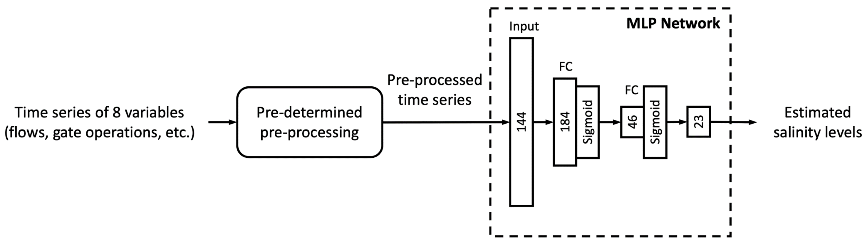
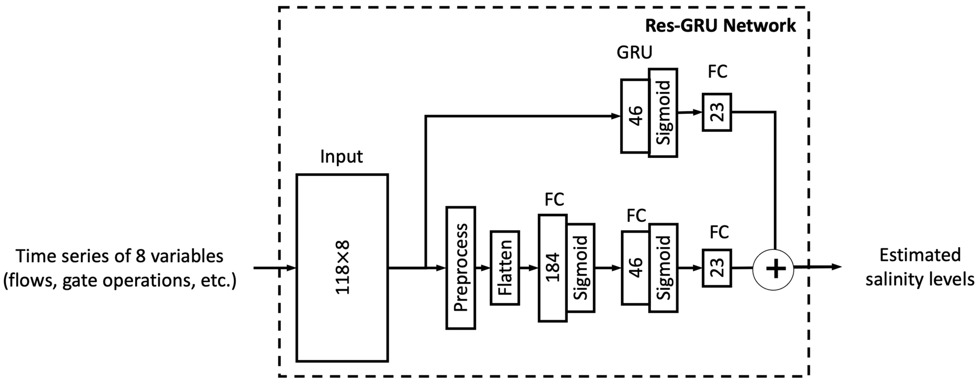
2.2. Machine Learning (ML) Models

The current study explores the usage of six different ML models in a multi-task learning framework (i.e., one ML model for all 23 study locations). The models include the baseline multi-layer perceptron (MLP) model and five other deep learning models: a Residual Network (ResNet), a Long-Short-Term Memory (LSTM) network, a Gated Recurrent Unit (GRU) network, a Residual LSTM (Res-LSTM), and a Residual GRU (Res-GRU). For simplicity, these models are described briefly as follows. Detailed information including schematics of model architectures on these six ML models can be found in [32,33].
The MLP model contains two fully connected (FC) hidden layers in addition to an input layer and an output layer (Figure A1 in Appendix A). The eight input features are pre-processed before being supplied to the MLP model. The ResNet model adds a shortcut connection to a main path formed by two convolutional layers, a flatten step and an FC layer (Figure A2). The shortcut path consists of an input flattening step and an FC layer. This design aims to skip the hand-crafted pre-processing step while preserving the temporal information in the input features. The recurrent neural network (RNN) is a type of ANN that can learn from input features’ temporal information. The LSTM network is a special type of RNN. Different from conventional RNNs, LSTM implements a “gate” concept and contains an input gate, a forget gate, and an output gate (Figure A3). This implementation makes it capable of storing a cell state vector that is maintained, updated, or erased when processing the input features recurrently. The GRU network is a different type of RNN but is less sophisticated when compared to an LSTM network in terms of structural complexity (Figure A4). A GRU network has only a reset gate and an update gate (rather than three gates in an LSTM network). It has no internal memory unit as an LSTM network does. Additionally, following the shortcut design in ResNet, we devise modified versions (with less complexity) of LSTM and GRU called Res-LSTM (Figure A5) and Res-GRU (Figure A6), respectively. To be specific, we use the MLP model as the main branch in Res-LSTM or Res-GRU but add the shortcut connection consisting of a single LSTM or GRU layer, which is less complex than the baseline LSTM or GRU architectures, to capture the residual between the reference salinity and the MLP-simulated salinity.

2.3. Study Metrics

To train the ML models, we utilize the widely used mean squared error as the loss function. To assess the performance of these ML models, we employ five commonly used statistical metrics: the mean squared error (MSE), the square of the correlation coefficient ( r 2 ), percent bias, root mean standard deviation ratio (RSR), and the Nash–Sutcliffe Efficiency (NSE) coefficient. These five metrics evaluate a model’s performance from different aspects and are complementary to each other. The MSE measures the average squared differences between the ML simulations and the targeted salinity, providing a quantifiable gauge of the magnitude of error in our model’s simulations; the r 2 metric sheds light on the strength of the linear relationship between ML simulations and the reference salinity; percent bias reveals whether a model overestimates or underestimates the reference salinity, and by how much on an average sense; RSR normalizes the root mean squared error between modeled and reference salinity using reference salinity’s standard deviation; NSE quantifies the general predictive skill of ML models. For r 2 and NSE, values closer to 1 designate better performance. For MSE, percent bias, and RSR, values closer to 0 represent better performance.

2.4. Model Training and Test

All the ML models are trained and tested under two scenarios: (a) trained using the first 70% of the observed salinity data and tested using the last 30% of the observed data; and (b) trained using the first 70% of the observed data plus the first eight scenarios (scenarios 1–8 in Table 1) of the augmented data and tested using the remaining four scenarios (scenarios 9–12 in Table 1). During the training process of both scenarios, we use the baseline data (baseline scenario in Table 1) without any manual manipulation of input features for validation. Specifically, we monitor the convergence of the model by computing the loss on this baseline dataset and we stop the training when validation loss stops decreasing for 50 epochs to minimize potential overfitting. This strategy is often called early stopping. It is a valuable regularization technique in machine learning that offers several advantages, as highlighted by various studies [47,48]. By halting the training process when the model’s performance on a validation dataset no longer improves, early stopping helps prevent overfitting, ensuring that the model generalizes well to unseen data [49]. Additionally, this strategy increases computational efficiency, reducing the number of training epochs and saving both time and resources, particularly when working with large datasets or complex models [50].
All the adopted ML models are trained using the Adam optimizer [51] with a fixed learning rate of 0.001 and a mini-batch size of 128. Training and testing are carried out on a public cloud-based platform: the Google Colaboratory.

2.5. Transfer Learning to Observed Data

Transfer learning is a widely used machine learning technique that capitalizes on the knowledge from pre-trained models to enhance performance on new tasks. In transfer learning, a model trained on one task is fine-tuned for another related task, allowing for faster training while achieving good performance with relatively little training data [39]. In the context of Delta salinity modeling, transfer learning, as opposed to training from scratch, involves (a) pre-training the model on augmented data, (b) re-initializing the output layer, and (c) fine-tuning the model using observed (new) data (Figure 2). The observed data include daily data for the 23 study locations, consistent with the original augmented training dataset.
The original pre-trained models gain sufficient knowledge on flow–salinity relationships from learning to emulate a wide range of DSM2-simulated outcomes. As a result, they can quickly adapt to real-world flow–salinity relationship patterns in historical data by reusing the knowledge it has already acquired on how to identify and handle different types of features. Specifically, models pre-trained on augmented simulation data are adapted for a similar task by randomly re-initializing the output layer and training all layers end-to-end on the training split of the observed data.
To retain the knowledge acquired during pre-training while fine-tuning the model, the learning rates of different layers are modified. In particular, the front layers’ learning rate is set to 0.1× the output layer’s learning rate, facilitating faster output layer training and ensuring the effective transfer and preservation of knowledge from the front layers. The optimal learning rate ratio (0.1) is determined through multiple experiments with varying ratios, among a finite set of 0.01, 0.1, 0.5, 1, and evaluating model performance on the test split of the observed data. This transfer learning approach enables the leveraging of pre-trained models for improved performance on observed data, benefiting from knowledge transfer between tasks while effectively adapting the model to new data.

2.6. Dashboard

A web-based Salinity Dashboard (Dashboard) is developed to serve as the front-end user interface for the machine learning salinity emulators described above. The Dashboard facilitates user interaction with the underlying ML models by allowing easy modification of the Delta boundary conditions (i.e., the input variables), such as Delta inflow, pumping, and salinity boundary conditions. The pre-trained ML models (using augmented data) are evaluated based on the user-modified inputs to the boundary conditions. The model is reevaluated with every user-directed change of the boundary conditions. The reevaluation of the ML models takes seconds, which allows for quick screening of multiple scenarios (e.g., varying water year types, flow conditions, boundary salinity conditions, pumping, etc.) in a web browser.

3. Results

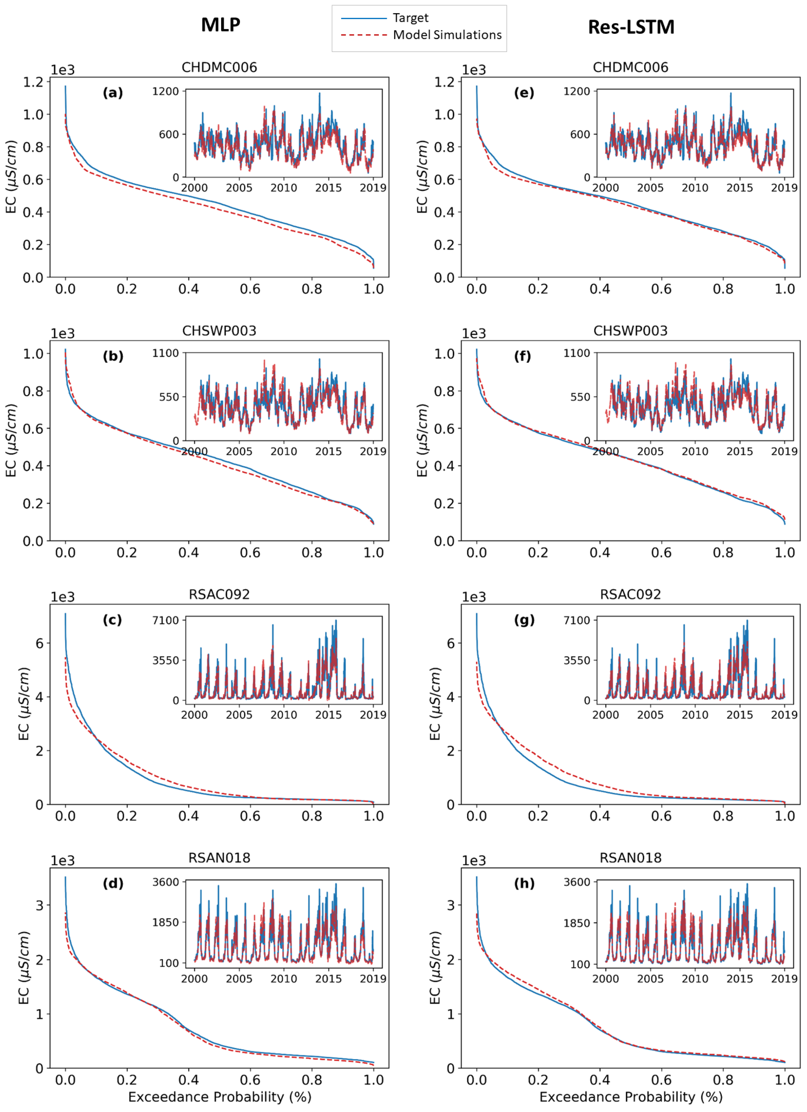
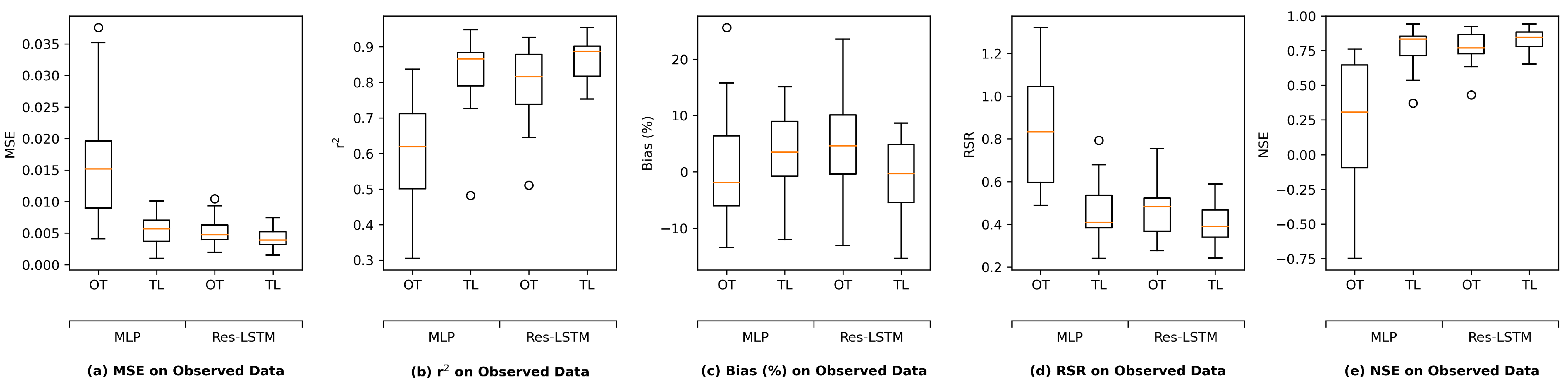
3.1. ANNs with Augmented Data

This section compares the performance of one adopted deep learning model, Res-LSTM, against the baseline machine learning model MLP. The results for the other four deep learning models utilized in the study are shown in Figure A7 in Appendix B. Figure 3 provides a visualization of the comparison using boxplots, enabling us to assess the performance metrics of the models under each condition. Figure 3 is organized into ten panels, labeled ‘(a)’ through ‘(j)’, with five panels in each row displaying the MSE, r 2 , Bias%, RSR, and NSE metrics, respectively. The first row (panels (a)–(e)) shows the results from testing the models on observed data, where the test dataset comprises the last 30% of the observed data. The second row (panels (f)–(j)) presents the results from testing the models on augmented data, the test dataset from scenarios 9–12 in Table 1. In each panel, we provide four boxplots representing the performance of MLP and Res-LSTM in the OT (trained using observed data only) and OAT (training using augmented and observed data) scenarios, respectively.
Examining the boxplots in Figure 3 allows us to draw a couple of key conclusions. When comparing the OAT boxplots with OT, based on the range and median of boxplots, OAT shows significantly better results than OT. For example, in panel (b), the median r 2 is about 0.6 for both Res-LSTM and MLP in the OT scenario, while it is approximately 0.90 for both models in the OAT scenario. Additionally, the OT scenario has a wider range than the OAT scenario. Similarly, the RSR of OT (Res-LSTM and MLP) in panel (d) is about 0.8, and for OAT, it is 0.38. The same pattern is observed for the second row of boxplots (panels (f)–(j)). For instance, the median r 2 in panel (g) is about 0.45 for the OT scenarios and 0.90 for the OAT scenarios, indicating that OAT has better performance than OT. Similar trends can be observed in panel (f) dedicated to MSE. The median MSE for OAT scenarios approximates 0, demonstrating superior performance compared to the OT scenarios, which show a median MSE of about 0.018. Furthermore, OT demonstrates larger variability compared to OAT, underscoring the more consistent and accurate performance achieved with the OAT approach. It is also notable that both MLP and Res-LSTM models have similar performance. However, the Res-LSTM model shows slightly better performance than the MLP model. This high-level analysis allows us to understand the effectiveness of the data-augmentation technique in improving the accuracy of salinity modeling using deep learning approaches.
Exceedance probability curves are graphical representations that help visualize and analyze the distribution of data. They can be used to compare model predictions with observed data in order to assess the model’s performance. Figure 4 displays exceedance probability curves and time series plots (in the insert plots) for the daily observed salinity and the corresponding simulations from Res-LSTM and MLP at four key locations under the OAT scenario. The x-axis represents the exceedance probability ranging from 0 to 1 (or 0% to 100%), and the y-axis represents the salinity (represented by EC) values. These locations serve important purposes in the transfer and management of water, consisting of two critical water-supply intake locations: HDMC006 (location #10 in Figure 1) and CHSWP003 (location #9 in Figure 1); and two locations that play a crucial role in maintaining compliance with salinity regulations: Emmaton (RSAC092; location #4 in Figure 1) and Jersey Point (RSAN018; location #8 in Figure 1).
The model curve (in dashed red line) being above the observed curve (in solid blue line) suggests that the model is overestimating the EC values. Conversely, the model curve being below the observed curve indicates that the model is underestimating the EC values. Figure 4 indicates that the exceedance probability curves for both models well resemble that of the observed salinity for the four study locations. Specifically, MLP slightly underestimates the salinity across all salinity ranges at the intake location CHDMC006 (panel (a)). In comparison, Res-LSTM only underestimates in the high-salinity range (>6000 μ S/cm) at this location (panel (b)). This is also evident in the insert time series plots. At the other intake location CHSWP003, Res-LSTM also outperforms MLP which underestimates the low-medium ranges of salinity (panels (c) and (d)). At the compliance locations Emmaton (panels (e) and (f)), the performance of both models is generally satisfactory but is relatively inferior compared to their performance at those two intake locations. Notably from the exceedance probability curves and time series plots, both models underestimate high range of salinity but overestimate low-medium range of salinity throughout the study period. The underestimation of high salinity is also clear at the other compliance location Jersey Point (panels (g) and (h)) for both models. However, different from Emmaton, both models, particularly the Res-LSTM model, simulate the low-medium range of salinity well at Jersey Point.
Overall, data augmentation leads to improved performance of both the baseline MLP model and the adopted deep learning models including Res-LSTM. The performance of the baseline MLP model is desirable. However, the other adopted deep learning models generally yield comparable or superior simulations of Delta salinity.

3.2. Transfer Learning

This section assesses the performance of models trained using the transfer learning technique described in Section 2.5. Figure 5 illustrates the statistical metrics for test performance of the MLP and Res-LSTM models. The MLP and Res-LSTM models were selected for comparison because MLP serves as the baseline model, and the Res-LSTM’s performance is generally in line with that of the four other models trained. Within each boxplot, the OT box represents the model trained on observed data and the TL box represents the transfer learned model.
Starting with panel (a), it examines MSE, where a lower value is indicative of better performance. For MLP, the MSE in the OT scenario has a broad range from 0.004 to 0.036, but is significantly reduced in the TL scenario, with a range from 0.002 to 0.01. Likewise, for Res-LSTM, the MSE in the OT scenario spans from 0.003 to 0.01, and narrows down to 0.002 to 0.008 in the TL scenario. Among all the models, the lowest median MSE is found with the Res-LSTM (TL) model, underscoring the superior performance of models leveraging transfer learning. In panel (b), concerning the r 2 values for MLP (OT) range from 0.3 to 0.83, and for Res-LSTM (OT), they stretch from 0.38 to 0.85. The range of r 2 for the transfer learned models (TL) is smaller than that of the (OT) models, approximately 0.75 to 0.97. Furthermore, the Res-LSTM (TL) model has a larger minimum r 2 value and a narrower range compared to the MLP (TL) model. In terms of bias (panel (c)), the TL model eliminates the apparent outlier (27% for MLP and 48% for Res-LSTM), learning for a narrow variation range across the study locations. Finally, panels (d) and (e) display the metrics for RSR and NSE, respectively. In these panels, we can observe narrower ranges for both RSR and NSE with more desirable median values for both MLP (TL) and Res-LSTM (TL).
In comparison to the models without transfer learning, the transfer learned models generally exhibit better performance, highlighting the effectiveness of transfer learning in enhancing the model’s ability to estimate salinity. The Res-LSTM model, when fine-tuned with transfer learning, demonstrates greater skill in salinity estimation, as the median values across all metrics are closer to the ideal values, and the variations are reduced. Similar improvements are observed in the other deep learning architectures, as depicted in Figure A8 in Appendix B. Notably, the performance of the transfer learned models is on par with the models trained with a combined augmented–observed dataset (Figure 3).

3.3. Dashboard

A complementary browser-based Delta Salinity Dashboard (Dashboard) was developed to serve as the front-end user interface for the DSM2 salinity emulators described in Section 2.6. This Dashboard evaluates pre-trained models based on user-modified inputs with no need to re-train the models. In this dashboard, users can interactively explore hypothetical scenarios and view the corresponding salinity outputs at key compliance locations during user-defined simulation periods.

3.3.1. Dashboard Architecture

The Dashboard is written in Python and uses several Python libraries, including TensorFlow, Panel, Bokeh, and Pandas. The pre-trained deep learning models (GRU, LSTM, ResNet, Res-GRU, and Res-LSTM) are evaluated by the Dashboard and the results are presented as a Pandas DataFrame object. Bokeh, a Python library for creating interactive visualizations, is used to plot the evaluated models. The plots and widgets are assembled in a dashboard layout using Panel, a Python library used for creating interactive web apps and dashboards by connecting user-defined widgets to plots, images, tables, or text.
The Dashboard is hosted on Azure using Azure Web App Service, which hosts a Linux Docker Container with the required dependencies. Docker packages software into standardized units called containers which include everything needed for the Dashboard to run, such as Python and its packages. The Dashboard Python code, pre-trained models, and input data templates are stored in a GitHub repository. Azure servers can be scaled up to improve virtual machine processing performance or scaled out to increase the number of virtual machines. This scaling can be adjusted based on the application’s resource needs and user traffic.

3.3.2. Dashboard Elements

The Dashboard is hosted on the cloud and accessible through a web link (accessed on 1 May 2023). (dwrbdodash.azurewebsites.net). Upon opening the link, the Dashboard will be displayed, as shown in Figure 6. The main elements of the Dashboard are highlighted in Figure 6 and further explained in Table 2.

3.3.3. Dashboard Example Use Case

This section demonstrates the Dashboard by simulating a critically dry year, 2015. The simulated scenario will use a version of 2015 hydrology that is modified to represent arbitrarily drier conditions (reduced winter peak inflows, spring runoff, and exports). The Dashboard configurations used to set up the scenario are shown in Figure 7.
The outcomes of the example simulation are shown in Figure 8 as the solid lines. Salinity results are shown at Sacramento River near Emmaton and San Joaquin River at Jersey Point, two important compliance locations for Delta water quality-control standards. Visual inspection of the Dashboard outputs indicates higher spring salinity resulting from the reduced inflows. Under the critically dry conditions simulated, a 15% decrease in March–May runoff increased the June EC by approximately 1000 μ S/cm at Emmaton (Figure A9 in Appendix B) and 500 μ S/cm at Jersey Point (Figure A10), compared to historical conditions. There was a minimal salinity response in December despite the 20% reduction of inflows, due to the relatively high flows that month.
Salinity simulations like the one in this case study are routinely conducted with process-based one-dimensional models of the Delta, such as DSM2. To verify its value as a DSM2 surrogate, it is appropriate to compare the results of the emulation with the results of DSM2 under the same input assumptions. Figure 8 shows the comparison between the emulator (Res-LSTM architecture) and a full-featured DSM2 run with the same hydrologic inputs from the example use case. Dashed lines represent the DSM2 simulations and solid lines represent the outcomes of the DSM2 emulator. Generally, the alignment between the emulator and DSM2 are close, supporting the concept that the emulator can be used as a screening tool.

4. Discussions

4.1. Implications

This study holds significant implications for water resource management and scientific exploration. The main contributions of the study and their potential applications are outlined below:
(a)
Data augmentation: The study demonstrates the effectiveness of data augmentation in addressing the challenge of limited historical measurements for data-driven deep learning models. This approach enhances the performance and versatility of machine learning models by providing a more diverse and representative dataset. In practical terms, the data-augmentation method can be applied to various scientific explorations, allowing researchers to tackle complex problems with limited data.
(b)
Transfer learning: The introduction of transfer learning allows knowledge gained from one problem to be applied to solve a related problem. This methodology can be adapted to simulate numerous other variables relevant to water resource management (e.g., water temperature, dissolved oxygen, turbidity, and ion constituents) and the same variables for other estuarine environments.
(c)
Continuous model evolution: Both the data augmentation and transfer learning methods aim to incorporate augmented data into the training process, achieving improvements over the baseline model trained using observed data alone. As hydrodynamic models, salinity observations, and regulatory constraints are constantly evolving, the ability to build upon previous knowledge through transfer learning allows machine learning models to continuously adapt to the changing state of science in the Delta.
(d)
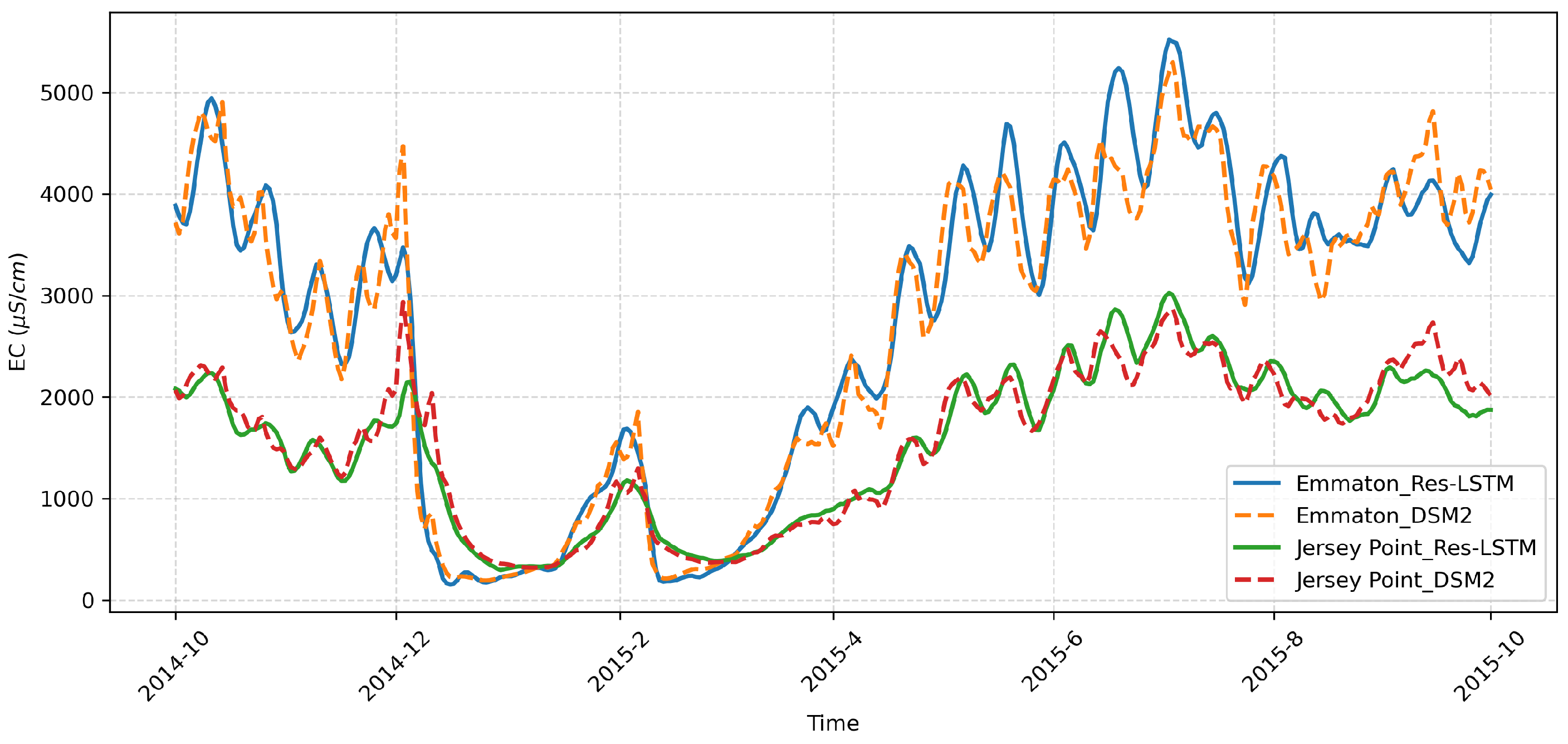
Machine learning-based Salinity Dashboard: The Salinity Dashboard is capable of estimating salinity data comparable to a full-featured DSM2 model. It has practical applications in real-time operations. By incorporating the Salinity Dashboard with real-time data, it can inform decision-making and improve water-management strategies. Furthermore, the efficient emulation facilitates sensitivity analyses in long-term planning studies, enabling researchers to conduct a higher number of scenario permutations.

4.2. Future Work

This study demonstrates the ability and applicability of deep learning in salinity modeling when combined with data augmentation and transfer learning. Specifically, in transfer learning, we trained models using augmented data and applied the trained model to observed data. In a follow-up study, we will apply the trained models in other tasks including salinity simulations under projected climate-change scenarios (e.g., sea level rise) which becomes increasingly indispensable in long-term water resource planning. In addition to transferability, we also plan to investigate the interpretability of the machine learning models. One way is to implement different explainable artificial intelligence (XAI [52]) approaches including backpropagation-based [53] and gradient-based [54] methods into machine learning models. Another way is to combine physical knowledge (e.g., salinity transport equations in process-based models) into machine learning models. The combined models are often called physics-informed neural networks (PINN [55,56,57]). In an ongoing study, we are developing PINNs to model salinity at a smaller group of study locations and comparing their performance against that of conventional neural networks. Preliminary results indicate that PINNs outperform conventional models notably. The corresponding findings will be reported in a separate paper.
The study also presents a prototype Delta Salinity Dashboard centered on the machine learning models adopted. The Dashboard will be continually improved with ongoing advancements to the underlying machining models and application needs. Ongoing and planned improvements to the dashboard include:
(a)
Improved utilities to modify the inputs: The Dashboard’s input modification utilities will be expanded beyond the current pre-set range. Future iterations will enable users to upload their own input datasets in various formats (e.g., text files) to provide more customized simulation scenarios.
(b)
Additional post-processing options: In addition to the current time series plots, the Dashboard’s outputs will be post-processed to include other useful formats such as exceedance plots and monthly averages.
(c)
Multi-year simulation: Instead of limiting the simulation to one year, future iterations of the Dashboard will allow for multiple years of simulation to facilitate the simulation of, for example, multi-year droughts.
(d)
Spatial output viewer: Incorporate a map view to show key metrics of all locations simultaneously.
(e)
Report renerator: Include an option to generate a template-based report with key indicators of Delta water quality.

5. Conclusions

This study explores the application of deep learning with data augmentation and transfer learning in salinity modeling for the Sacramento-San Joaquin Delta. From a scientific point of view, the study was the first attempt to (a) develop state-of-the-art deep learning models using augmented data in the study area; and (b) assess the feasibility of transferring pre-trained deep learning models to a different problem. The results demonstrated the effectiveness and efficiency of data augmentation and transfer learning in providing satisfactory salinity simulations across the Delta. This lays the foundation for us to further explore other important management variables (via transfer learning) and tackle other problems with limited data available (via data augmentation). Additionally, the ability to build upon previous knowledge through transfer learning allows deep learning models to continuously adapt to the changing state of science in the Delta. From a practical standpoint, the study developed a user-friendly salinity modeling dashboard that runs much faster (e.g., in seconds) than conventional process-based models (e.g., in hours). The dashboard can be applied in real time to quickly assess the impacts of different operational scenarios and select the optimal operation. The dashboard can also facilitate sensitivity analysis in long-term planning studies, allowing the users to conduct a higher number of scenario permutations in a timely manner.
Despite these advances, the study exemplified the transferability of the deep learning models developed via a single task (i.e., transfer from simulated to observed data). In our follow-up studies, we will apply the transfer learning technique to other tasks including climate change-induced saline seawater intrusion which becomes increasingly indispensable in long-term water resource-planning studies. Furthermore, the interpretability of the deep learning models proposed is not assessed as it is outside the scope of the current study. In follow-up studies, we plan to explore various explainable artificial intelligence techniques to shed light on the interpretability of the models. Finally, the salinity-simulation dashboard developed in the current study was meant to be a prototype. In the future, we will continually improve the dashboard with ongoing advancements to the underlying machining models and application needs.

Author Contributions

Conceptualization, P.S., Z.B., Z.D. and M.H.; Data curation, B.T., R.H., P.N. and Y.Z.; Funding acquisition, P.S.; Investigation, S.Q., R.H. and M.H.; Methodology, S.Q., R.H., M.H., Z.B., Z.D., P.S. and J.A.; Project administration, P.S.; Software, S.Q. and R.H.; Validation, M.H., R.H., P.N., Y.Z., V.H. and D.M.R.; Visualization, S.Q., M.H.; Writing—original draft, S.Q., M.H., Y.Z., B.T., R.H., P.N. and J.A.; Writing—review and editing, Z.B., P.S., J.A., F.C., V.H. and D.M.R. All authors have read and agreed to the published version of the manuscript.

Funding

This research was funded by the California Department of Water Resources and the University of California, Davis grant number 4600014165-01.

Data Availability Statement

The datasets used and scripts (in Python) developed in the current study are uploaded to a GitHub repository and are available from the corresponding author on reasonable request.

Acknowledgments

The authors would like to thank the editors and three anonymous reviewers for providing thoughtful and insightful comments that helped to improve the quality of this study. The views expressed in this paper are those of the authors, and not of the State of California.

Conflicts of Interest

The authors declare no conflict of interest.

Appendix A. Machine Learning Architectures

Figure A1. Schematic of the MLP network from [32]. The number in the input layer denotes input shape and those in the subsequent FC layers represent the numbers of neurons of the layers.
Water 15 02482 g0a1
Figure A2. Schematic of the ResNet network from [32]. The number in the input layer denotes input shape and those in the FC layers represent the numbers of units/neurons of the layers. In the convolutional layers following the input layer, “f” denotes the number of convolutional filters, “k” denotes size of convolutional kernels and “s” denotes stride.
Water 15 02482 g0a2
Figure A3. Schematic of the LSTM network from [32]. The number in the input layer denotes input shape and those in the subsequent layers represent the numbers of units/neurons of the layers.
Water 15 02482 g0a3
Figure A4. Schematic of the GRU network from [32]. The number in the input layer denotes input shape and those in the subsequent layers represent the numbers of units/neurons of the layers.
Water 15 02482 g0a4
Figure A5. Schematic of the Res-LSTM network from [32]. The number in the input layer denotes input shape and those in the subsequent layers represent the numbers of units/neurons of the layers.
Water 15 02482 g0a5
Figure A6. Schematic of the Res-GRU network proposed in [33]. The number in the input layer denotes input shape and those in the subsequent layers represent the numbers of units/neurons of those layers.
Water 15 02482 g0a6

Appendix B. Additional Results

Figure A7. Test results of GRU, LSTM, Res-GRU, and ResNet architectures on the observed data (top row) and augmented data (bottom row).
Water 15 02482 g0a7
Figure A8. Transfer learning test results for GRU, LSTM, Res-GRU, and ResNet architectures.
Water 15 02482 g0a8
Figure A9. Output from the Dashboard showing salinity (represented by EC) at Emmaton resulting from modified Northern Flow and Pumping, per an example use case.
Water 15 02482 g0a9
Figure A10. Output from the Dashboard showing salinity (represented by EC) at Jersey Point resulting from modified inputs to Northern Flow and Pumping, per an example use case.
Water 15 02482 g0a10

References

  1. Alber, M. A conceptual model of estuarine freshwater inflow management. Estuaries 2002, 25, 1246–1261. [Google Scholar] [CrossRef]
  2. Water Resilience Portfolio; California Natural Resources Agency: Sacramento, CA, USA, 2020; p. 141.
  3. Moyle, P.B.; Brown, L.R.; Durand, J.R.; Hobbs, J.A. Delta smelt: Life history and decline of a once-abundant species in the San Francisco Estuary. San Fr. Estuary Watershed Sci. 2016, 14. [Google Scholar] [CrossRef]
  4. Rath, J.S.; Hutton, P.H.; Chen, L.; Roy, S.B. A hybrid empirical-Bayesian artificial neural network model of salinity in the San Francisco Bay-Delta estuary. Environ. Model. Softw. 2017, 93, 193–208. [Google Scholar] [CrossRef]
  5. Gude, V.G. Desalination of deep groundwater aquifers for freshwater supplies–Challenges and strategies. Groundw. Sustain. Dev. 2018, 6, 87–92. [Google Scholar] [CrossRef]
  6. Dhakal, N.; Salinas-Rodriguez, S.G.; Hamdani, J.; Abushaban, A.; Sawalha, H.; Schippers, J.C.; Kennedy, M.D. Is desalination a solution to freshwater scarcity in developing countries? Membranes 2022, 12, 381. [Google Scholar] [CrossRef] [PubMed]
  7. Abdelfattah, M.; Abu-Bakr, H.A.A.; Mewafy, F.M.; Hassan, T.M.; Geriesh, M.H.; Saber, M.; Gaber, A. Hydrogeophysical and hydrochemical assessment of the northeastern coastal aquifer of Egypt for desalination suitability. Water 2023, 15, 423. [Google Scholar] [CrossRef]
  8. Cooley, H.; Ajami, N. Key Issues for Seawater Desalination in California: Cost and Financing; Pacific Institute: Oakland, CA, USA, 2012; pp. 1–48. [Google Scholar]
  9. Meng, M.; Chen, M.; Sanders, K.T. Evaluating the feasibility of using produced water from oil and natural gas production to address water scarcity in California’s Central Valley. Sustainability 2016, 8, 1318. [Google Scholar] [CrossRef]
  10. Badiuzzaman, P.; McLaughlin, E.; McCauley, D. Substituting freshwater: Can ocean desalination and water recycling capacities substitute for groundwater depletion in California? J. Environ. Manag. 2017, 203, 123–135. [Google Scholar] [CrossRef]
  11. He, M.; Zhong, L.; Sandhu, P.; Zhou, Y. Emulation of a process-based salinity generator for the sacramento–San Joaquin Delta of california via deep learning. Water 2020, 12, 2088. [Google Scholar] [CrossRef]
  12. CDWR. Minimum Delta Outflow Program. In Methodology for Flow and Salinity Estimates in the Sacramento–San Joaquin Delta and Suisun Marsh: 11th Annual Progress Report; CDWR: Sacramento, CA, USA, 1990. [Google Scholar]
  13. Denton, R.A. Accounting for antecedent conditions in seawater intrusion modeling—Applications for the San Francisco Bay-Delta. Hydraul. Eng. 1993, 1, 448–453. [Google Scholar]
  14. Hutton, P.H.; Rath, J.S.; Chen, L.; Ungs, M.J.; Roy, S.B. Nine decades of salinity observations in the San Francisco Bay and Delta: Modeling and trend evaluations. J. Water Resour. Plan. Manag. 2016, 142, 04015069. [Google Scholar] [CrossRef]
  15. CDWR. Calibration and verification of DWRDSM. In Methodology for Flow and Salinity Estimates in the Sacramento–San Joaquin Delta and Suisun Marsh: 12th Annual Progress Report; CDWR: Sacramento, CA, USA, 1991. [Google Scholar]
  16. Cheng, R.T.; Casulli, V.; Gartner, J.W. Tidal, residual, intertidal mudflat (TRIM) model and its applications to San Francisco Bay, California. Estuarine Coast. Shelf Sci. 1993, 36, 235–280. [Google Scholar] [CrossRef]
  17. DeGeorge, J.F. A Multi-Dimensional Finite Element Transport Model Utilizing a Characteristic-Galerkin Algorithm; University of California: Davis, CA, USA, 1996. [Google Scholar]
  18. Casulli, V.; Zanolli, P. Semi-implicit numerical modeling of nonhydrostatic free-surface flows for environmental problems. Math. Comput. Model. 2002, 36, 1131–1149. [Google Scholar] [CrossRef]
  19. MacWilliams, M.; Bever, A.J.; Foresman, E. 3-D simulations of the San Francisco Estuary with subgrid bathymetry to explore long-term trends in salinity distribution and fish abundance. San Franc. Estuary Watershed Sci. 2016, 14. [Google Scholar] [CrossRef]
  20. CDWR. Bay-Delta SCHISM: A Framework for Decision Support in the Sacramento San Joaquin Delta. In Methodology for Flow and Salinity Estimates in the Sacramento–San Joaquin Delta and Suisun Marsh: 36th Annual Progress Report; CDWR: Sacramento, CA, USA, 2015. [Google Scholar]
  21. Chao, Y.; Farrara, J.D.; Zhang, H.; Zhang, Y.J.; Ateljevich, E.; Chai, F.; Davis, C.O.; Dugdale, R.; Wilkerson, F. Development, implementation, and validation of a modeling system for the San Francisco Bay and Estuary. Estuarine Coast. Shelf Sci. 2017, 194, 40–56. [Google Scholar] [CrossRef]
  22. Gaagai, A.; Aouissi, H.A.; Bencedira, S.; Hinge, G.; Athamena, A.; Heddam, S.; Gad, M.; Elsherbiny, O.; Elsayed, S.; Eid, M.H.; et al. Application of water quality indices, machine learning approaches, and GIS to identify groundwater quality for irrigation purposes: A case study of Sahara Aquifer, Doucen Plain, Algeria. Water 2023, 15, 289. [Google Scholar] [CrossRef]
  23. Gad, M.; Saleh, A.H.; Hussein, H.; Elsayed, S.; Farouk, M. Water Quality Evaluation and Prediction Using Irrigation Indices, Artificial Neural Networks, and Partial Least Square Regression Models for the Nile River, Egypt. Water 2023, 15, 2244. [Google Scholar] [CrossRef]
  24. Gad, M.; Gaagai, A.; Eid, M.H.; Szucs, P.; Hussein, H.; Elsherbiny, O.; Elsayed, S.; Khalifa, M.M.; Moghanm, F.S.; Moustapha, M.E.; et al. Groundwater Quality and Health Risk Assessment Using Indexing Approaches, Multivariate Statistical Analysis, Artificial Neural Networks, and GIS Techniques in El Kharga Oasis, Egypt. Water 2023, 15, 1216. [Google Scholar] [CrossRef]
  25. Sandhu, N.; Finch, R. Application of artificial neural networks to the Sacramento-San Joaquin Delta. In Estuarine and Coastal Modeling; ASCE: Reston, FL, USA, 1995; pp. 490–504. [Google Scholar]
  26. Wilbur, R.; Munevar, A. Integration of CALSIM and Artificial Neural Networks Models for Sacramento–San Joaquin Delta Flow-Salinity Relationships. In Methodology for Flow and Salinity Estimates in the Sacramento–San Joaquin Delta and Suisun Marsh: 22nd Annual Progress Report; CDWR: Sacramento, CA, USA, 2001. [Google Scholar]
  27. Mierzwa, M. CALSIM versus DSM2 ANN and G-model Comparisons. In Methodology for Flow and Salinity Estimates in the Sacramento–San Joaquin Delta and Suisun Marsh: 23rd Annual Progress Report; CDWR: Sacramento, CA, USA, 2002. [Google Scholar]
  28. Seneviratne, S.; Wu, S. Enhanced Development of Flow-Salinity Relationships in the Delta Using Artificial Neural Networks: Incorporating Tidal Influence. In Methodology for Flow and Salinity Estimates in the Sacramento–San Joaquin Delta and Suisun Marsh: 28th Annual Progress Report; CDWR: Sacramento, CA, USA, 2007. [Google Scholar]
  29. Jayasundara, N.C.; Seneviratne, S.A.; Reyes, E.; Chung, F.I. Artificial neural network for Sacramento–San Joaquin Delta flow–salinity relationship for CalSim 3.0. J. Water Resour. Plan. Manag. 2020, 146, 04020015. [Google Scholar] [CrossRef]
  30. Chen, L.; Roy, S.B.; Hutton, P.H. Emulation of a process-based estuarine hydrodynamic model. Hydrol. Sci. J. 2018, 63, 783–802. [Google Scholar] [CrossRef]
  31. Qi, S.; Bai, Z.; Ding, Z.; Jayasundara, N.; He, M.; Sandhu, P.; Seneviratne, S.; Kadir, T. Enhanced Artificial Neural Networks for Salinity Estimation and Forecasting in the Sacramento–San Joaquin Delta of California. J. Water Resour. Plan. Manag. 2021, 147, 04021069. [Google Scholar] [CrossRef]
  32. Qi, S.; He, M.; Bai, Z.; Ding, Z.; Sandhu, P.; Zhou, Y.; Namadi, P.; Tom, B.; Hoang, R.; Anderson, J. Multi-Location Emulation of a Process-Based Salinity Model Using Machine Learning. Water 2022, 14, 2030. [Google Scholar] [CrossRef]
  33. Qi, S.; He, M.; Bai, Z.; Ding, Z.; Sandhu, P.; Chung, F.; Namadi, P.; Zhou, Y.; Hoang, R.; Tom, B.; et al. Novel Salinity Modeling Using Deep Learning for the Sacramento–San Joaquin Delta of California. Water 2022, 14, 3628. [Google Scholar] [CrossRef]
  34. Wen, Q.; Sun, L.; Yang, F.; Song, X.; Gao, J.; Wang, X.; Xu, H. Time series data augmentation for deep learning: A survey. arXiv 2020, arXiv:2002.12478. [Google Scholar]
  35. Bandara, K.; Hewamalage, H.; Liu, Y.H.; Kang, Y.; Bergmeir, C. Improving the accuracy of global forecasting models using time series data augmentation. Pattern Recognit. 2021, 120, 108148. [Google Scholar] [CrossRef]
  36. Wang, F.; Tian, D.; Lowe, L.; Kalin, L.; Lehrter, J. Deep learning for daily precipitation and temperature downscaling. Water Resour. Res. 2021, 57, e2020WR029308. [Google Scholar] [CrossRef]
  37. Kim, H.I.; Han, K.Y. Urban flood prediction using deep neural network with data augmentation. Water 2020, 12, 899. [Google Scholar] [CrossRef]
  38. Li, X.; Grandvalet, Y.; Davoine, F.; Cheng, J.; Cui, Y.; Zhang, H.; Belongie, S.; Tsai, Y.H.; Yang, M.H. Transfer learning in computer vision tasks: Remember where you come from. Image Vis. Comput. 2020, 93, 103853. [Google Scholar] [CrossRef]
  39. Gopalakrishnan, K.; Khaitan, S.K.; Choudhary, A.; Agrawal, A. Deep convolutional neural networks with transfer learning for computer vision-based data-driven pavement distress detection. Constr. Build. Mater. 2017, 157, 322–330. [Google Scholar] [CrossRef]
  40. Brodzicki, A.; Piekarski, M.; Kucharski, D.; Jaworek-Korjakowska, J.; Gorgon, M. Transfer learning methods as a new approach in computer vision tasks with small datasets. Found. Comput. Decis. Sci. 2020, 45, 179–193. [Google Scholar] [CrossRef]
  41. Ruder, S.; Peters, M.E.; Swayamdipta, S.; Wolf, T. Transfer learning in natural language processing. In Proceedings of the 2019 Conference of the North American Chapter of the Association for Computational Linguistics: Tutorials; 2019; pp. 15–18. Available online: https://www.ruder.io/state-of-transfer-learning-in-nlp/ (accessed on 1 May 2023).
  42. Sullivan, P.; Shibano, T.; Abdul-Mageed, M. Improving automatic speech recognition for non-native english with transfer learning and language model decoding. arXiv 2022, arXiv:2202.05209. [Google Scholar]
  43. Mamyrbayev, O.; Alimhan, K.; Oralbekova, D.; Bekarystankyzy, A.; Zhumazhanov, B. Identifying the influence of transfer learning method in developing an end-to-end automatic speech recognition system with a low data level. East.-Eur. J. Enterp. Technol. 2022, 1, 84–92. [Google Scholar] [CrossRef]
  44. Willard, J.D.; Read, J.S.; Appling, A.P.; Oliver, S.K.; Jia, X.; Kumar, V. Predicting water temperature dynamics of unmonitored lakes with meta-transfer learning. Water Resour. Res. 2021, 57, e2021WR029579. [Google Scholar] [CrossRef]
  45. Zhao, X.; Luo, T.; Jin, H. Predicting diffusion coefficients of binary and ternary supercritical water mixtures via machine and transfer learning with deep neural network. Ind. Eng. Chem. Res. 2022, 61, 8542–8550. [Google Scholar] [CrossRef]
  46. Kimura, N.; Yoshinaga, I.; Sekijima, K.; Azechi, I.; Baba, D. Convolutional neural network coupled with a transfer-learning approach for time-series flood predictions. Water 2019, 12, 96. [Google Scholar] [CrossRef]
  47. Prechelt, L. Automatic early stopping using cross validation: Quantifying the criteria. Neural Netw. 1998, 11, 761–767. [Google Scholar] [CrossRef]
  48. Goodfellow, I.; Bengio, Y.; Courville, A. Deep Learning; MIT Press: Cambridge, MA, USA, 2016. [Google Scholar]
  49. Yao, Y.; Rosasco, L.; Caponnetto, A. On early stopping in gradient descent learning. Constr. Approx. 2007, 26, 289–315. [Google Scholar] [CrossRef]
  50. Srivastava, N.; Hinton, G.; Krizhevsky, A.; Sutskever, I.; Salakhutdinov, R. Dropout: A simple way to prevent neural networks from overfitting. J. Mach. Learn. Res. 2014, 15, 1929–1958. [Google Scholar]
  51. Kingma, D.P.; Ba, J. Adam: A method for stochastic optimization. arXiv 2014, arXiv:1412.6980. [Google Scholar]
  52. Adadi, A.; Berrada, M. Peeking inside the black-box: A survey on explainable artificial intelligence (XAI). IEEE Access 2018, 6, 52138–52160. [Google Scholar] [CrossRef]
  53. Shrikumar, A.; Greenside, P.; Kundaje, A. Learning important features through propagating activation differences. In International Conference on Machine Learning; PMLR: Sydney, Australia, 2017; pp. 3145–3153. [Google Scholar]
  54. Ancona, M.; Ceolini, E.; Öztireli, C.; Gross, M. Towards better understanding of gradient-based attribution methods for deep neural networks. arXiv 2017, arXiv:1711.06104. [Google Scholar]
  55. Lu, L.; Meng, X.; Mao, Z.; Karniadakis, G.E. DeepXDE: A deep learning library for solving differential equations. SIAM Rev. 2021, 63, 208–228. [Google Scholar] [CrossRef]
  56. Raissi, M.; Perdikaris, P.; Karniadakis, G.E. Physics-informed neural networks: A deep learning framework for solving forward and inverse problems involving nonlinear partial differential equations. J. Comput. Phys. 2019, 378, 686–707. [Google Scholar] [CrossRef]
  57. Roh, D.M.; He, M.; Bai, Z.; Sandhu, P.; Chung, F.; Ding, Z.; Qi, S.; Zhou, Y.; Hoang, R.; Namadi, P.; et al. Physics-Informed Neural Networks-Based Salinity Modeling in the Sacramento–San Joaquin Delta of California. Water 2023, 15, 2320. [Google Scholar] [CrossRef]
Figure 1. Schematic showing locations of modeled and observed salinity data used in the study.
Water 15 02482 g001
Figure 2. Diagram showing the transfer learning process.
Water 15 02482 g002
Figure 3. Boxplots showing statistical metrics of test results of MLP and Res-LSTM on the observed data (top row) and augmented data (bottom row).
Water 15 02482 g003
Figure 4. Exceedance probability curves and time series plots of daily salinity at four key study locations of OAT trained MLP model (a) CHDMC006, (b) CHSWP003, (c) RSAC092, (d) RSAN018, and Res-LSTM model (e) CHDMC006, (f) CHSWP003, (g) RSAC092, (h) RSAN018, to compare with the observed data.
Water 15 02482 g004
Figure 5. Box plots showing the statistical metrics for test performance of the observed data-trained (OT) and transfer learned (TL) MLP and Res-LSTM models.
Water 15 02482 g005
Figure 6. Screenshot of the Dashboard, highlighting the interactive elements.
Water 15 02482 g006
Figure 7. Dashboard configurations for example use case.
Water 15 02482 g007
Figure 8. Outputs of the Res-LSTM model compared to DSM2 outputs for Sacramento River at Emmaton and San Joaquin River at Jersey Point.
Water 15 02482 g008
Table 1. DSM2 scenarios utilized to augment the historical data.
Scenario IndexScenario Description
BaselineHistorical DSM2 run from 1990 to 2019
1Historical DSM2 run with Sacramento River inflows shifted forward by 15 days
2Historical DSM2 run with Sacramento River inflows shifted backward by 15 days
3Historical DSM2 run with Sacramento River inflows scaled down by 20%
4Historical DSM2 run with Sacramento River inflows scaled up by 20%
5Historical DSM2 run with San Joaquin River inflows shifted forward by 15 days
6Historical DSM2 run with San Joaquin River inflows shifted backward by 15 days
7Historical DSM2 run with San Joaquin River inflows scaled down by 20%
8Historical DSM2 run with San Joaquin River inflows scaled up by 20%
9Historical DSM2 run with Delta Cross Channel Gates closed all the time
10Historical DSM2 run with Delta Cross Channel Gates open all the time
11Historical DSM2 run with Suisun Marsh Salinity Control Gates closed all the time
12Historical DSM2 run with Suisun Marsh Salinity Control Gates open all the time
Table 2. Description of the interactive dashboard elements.
Dashboard ElementDescription
1. Water Year SelectorSelect the water year for simulation. This tool simulates one water year at a time, where antecedent inputs are assumed to be historical conditions. Note: the modified inputs are not saved in memory. For example, if a user modifies the inputs for 2014, and then changes the simulation to 2015, the scaling factors for 2014 are reverted to historical conditions and 2015 inputs will be modified to reflect the scaling configurations shown on the Dashboard.
2. Input Location SelectorSelect the boundary input to modify. This dashboard supports the modification of major Delta boundary conditions, including Northern Flows, Pumping, San Joquin River Flow, and EC boundaries for the San Joaquin River and Sacramento River. Refer to Table 1 in [33] for descriptions of the input features.
3. Input ScalerSliders to scale the selected Delta boundary condition ± 20 % from the baseline (historical) values. The values shown next to the slider for each month indicate the scale factor. The scale factor uniformly scales the daily values of the boundary condition for a given month. The default scale factor of 1 sets the inputs equal to historical conditions for that month. A scale factor of 1.2 uniformly scales the daily values of that month to 120% of historical values and a scale factor of 0.8 uniformly scales the daily values of that month to 80% of historical values.
4. Input Data PlotPlot of the input features. The blue line indicates the user-modified (i.e., scaled) input feature and the light grey line shows the historical value.
5. Output Location SelectorSelect the output location for which to display outputs. Key water quality locations (including compliance locations) are included. See Figure 1 for details of the available output locations.
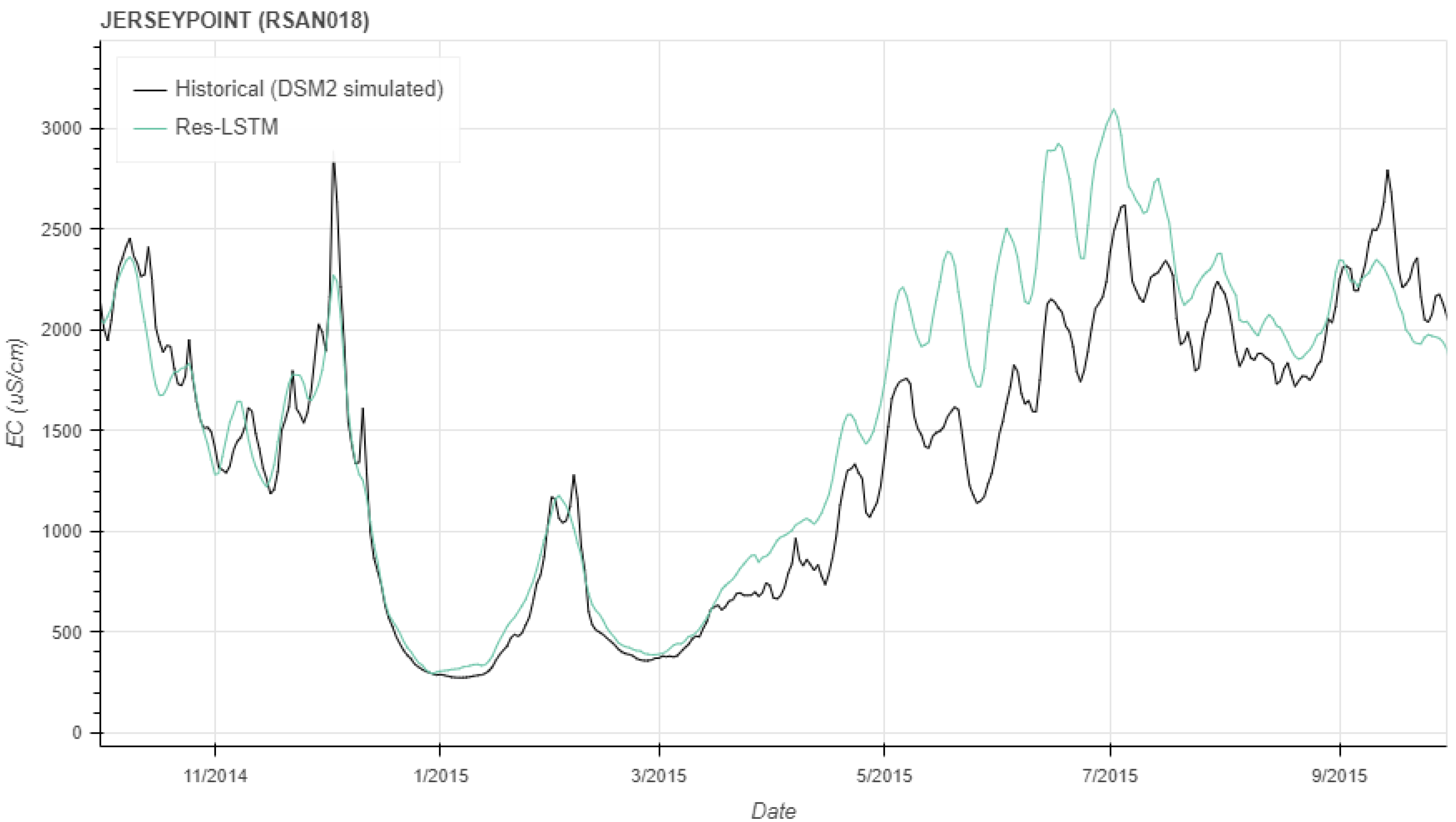
6. Output Location Salinity PlotPlot of the output locations. The black line represents the historical DSM2 simulation, and the various colored lines represent the outcomes from the salinity emulator, based on the user-modified inputs.
7. Machine Learning Architecture SelectionSelect the architectures to use in the emulator. See Section 2.2 for details.
8. Data Export OptionsOptions to export the inputs and outputs of the simulation in .csv format for the selected water year.
Disclaimer/Publisher’s Note: The statements, opinions and data contained in all publications are solely those of the individual author(s) and contributor(s) and not of MDPI and/or the editor(s). MDPI and/or the editor(s) disclaim responsibility for any injury to people or property resulting from any ideas, methods, instructions or products referred to in the content.

