

Evaluating Surface Water Nitrogen Pollution via Visual Clustering in Megacity Chengdu

 ,
,
Abstract
1. Introduction
2. Materials and Methods
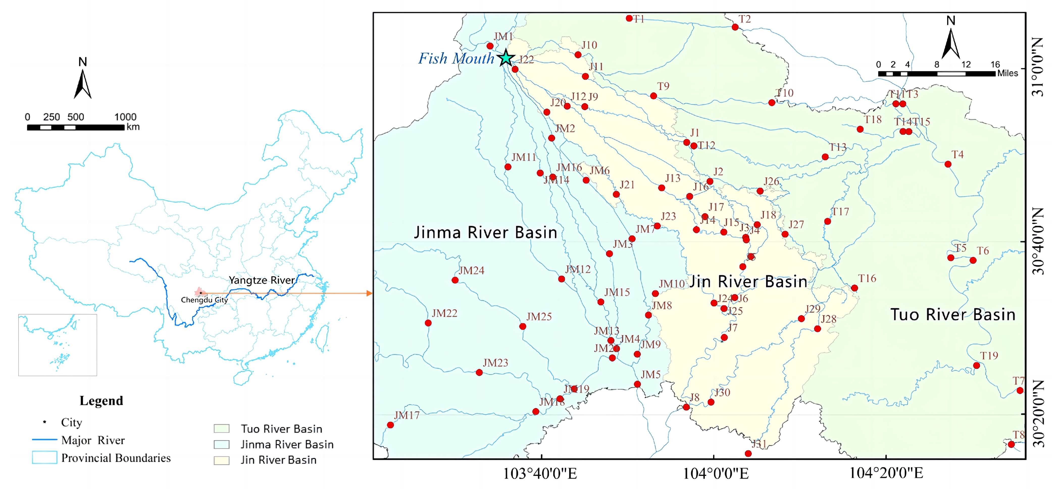
2.1. Study Area
2.2. Sample Collection
2.3. Chemometrics
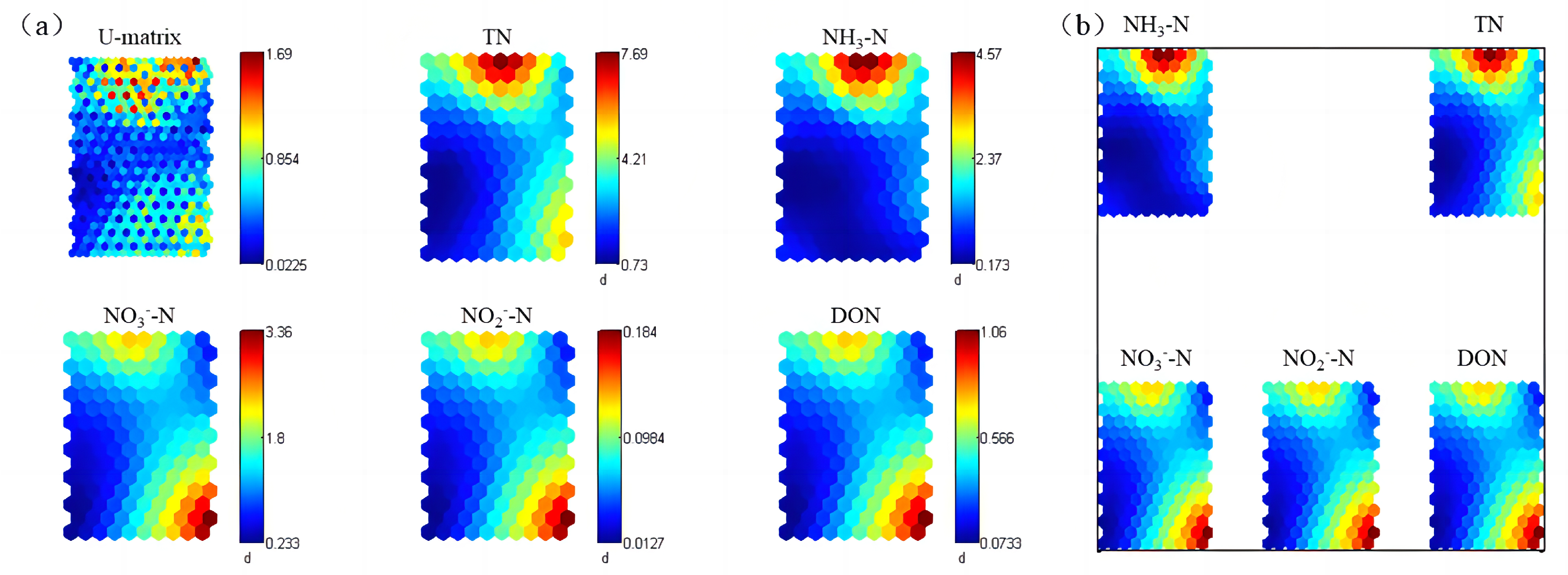
2.3.1. SOMs
2.3.2. HDT
3. Results
3.1. SOM Clustering Results
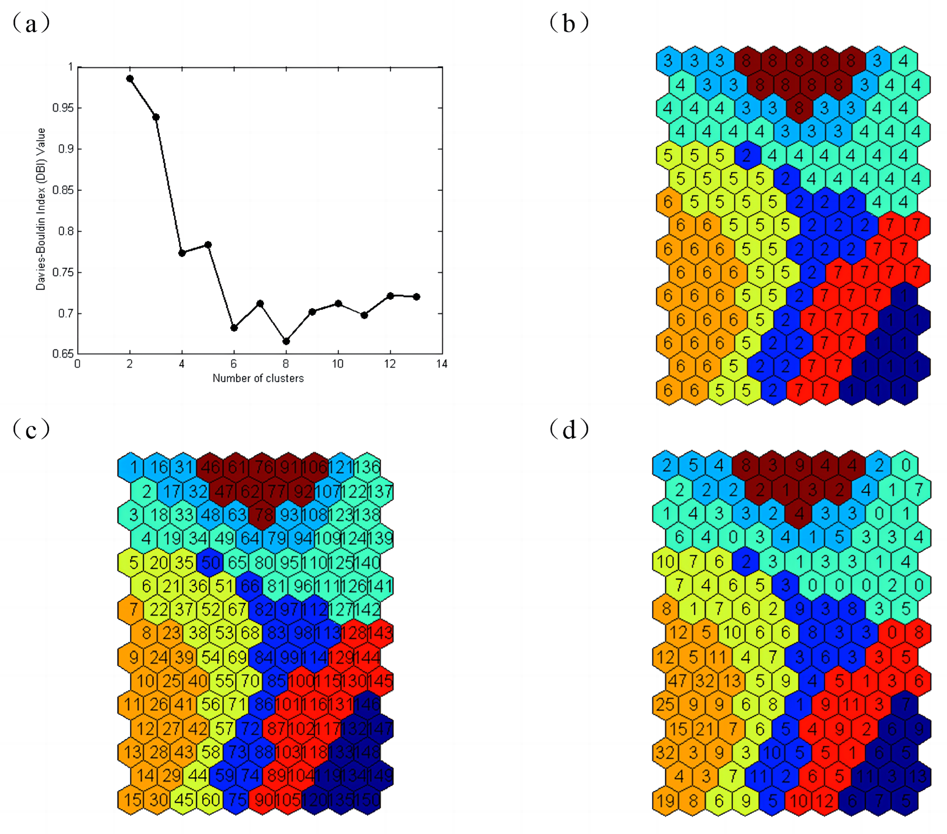
3.1.1. Determining the SOM Clustering Structure
3.1.2. Evaluation Index Selection
3.1.3. SOM Clustering Results
3.2. HDT Clustering Results
3.2.1. Determining the Data Set Equivalence Class and Evaluation Index Weight Ranking
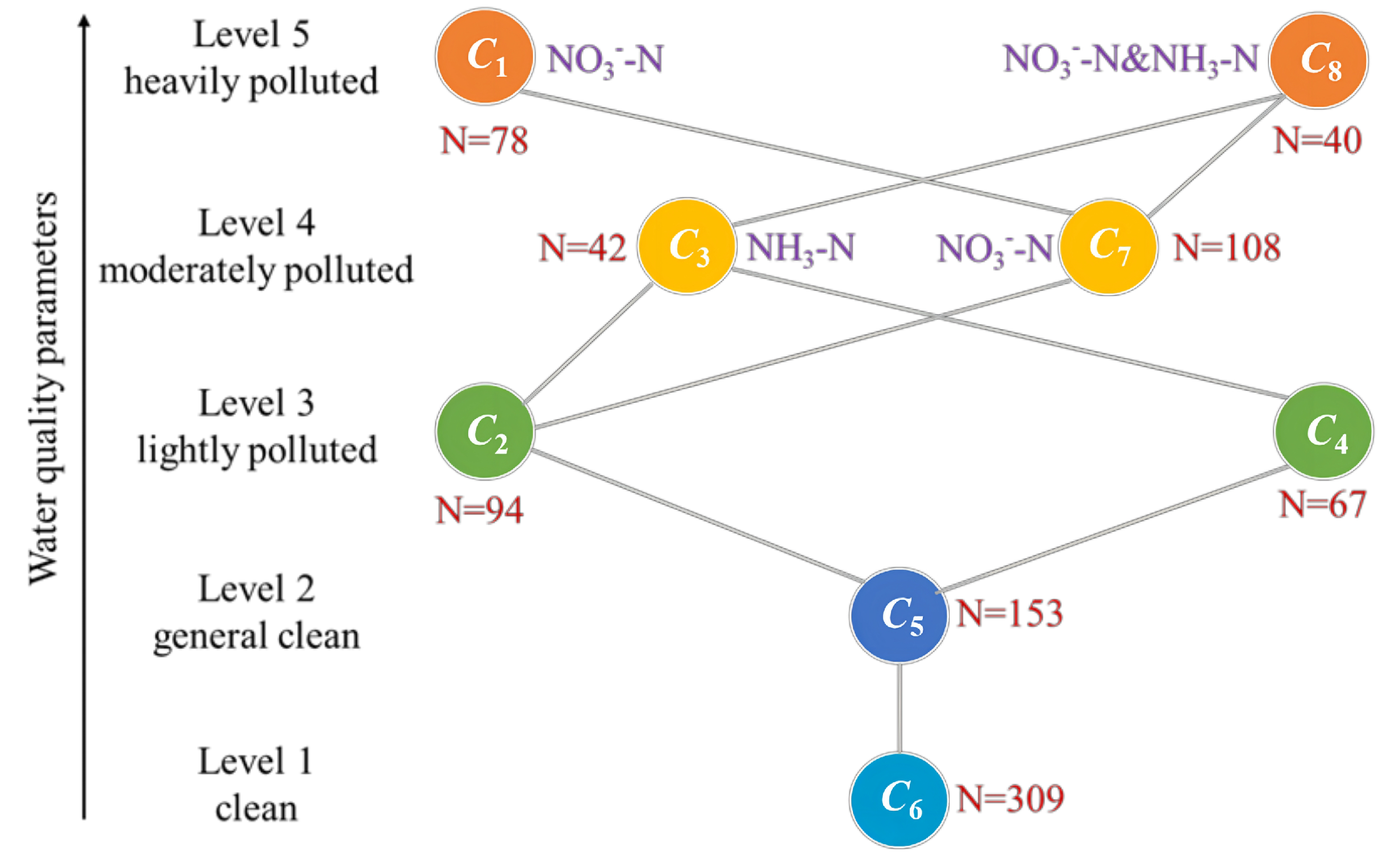
3.2.2. HDT Clustering Ranking
4. Discussion
4.1. Comprehensive Evaluation of Nitrogen Pollution
4.2. Advantages and Disadvantages of SOMs and HDT Technology
5. Conclusions
Author Contributions
Funding
Institutional Review Board Statement
Informed Consent Statement
Data Availability Statement
Acknowledgments
Conflicts of Interest
References
- Chen, J.; Chen, S.; Fu, R.; Li, D.; Jiang, H.; Wang, C.; Peng, Y.; Jia, K.; Hicks, B.J. Remote Sensing Big Data for Water Environment Monitoring: Current Status, Challenges, and Future Prospects. Earth’s Future 2022, 10, e2021EF002289. [Google Scholar] [CrossRef]
- Tang, W.; Pei, Y.; Zheng, H.; Zhao, Y.; Shu, L.; Zhang, H. Twenty years of China’s water pollution control: Experiences and challenges. Chemosphere 2022, 295, 133875. [Google Scholar] [CrossRef] [PubMed]
- Horton, R.K. An index number system for rating water quality. J. Water Pollut. Control Fed. 1965, 37, 300–306. [Google Scholar]
- Uddin, M.G.; Nash, S.; Rahman, A.; Olbert, A.I. A comprehensive method for improvement of water quality index (WQI) models for coastal water quality assessment. Water Res. 2022, 219, 118532. [Google Scholar] [CrossRef] [PubMed]
- Zeng, Q.; Luo, X.; Yan, F. The pollution scale weighting model in water quality evaluation based on the improved fuzzy variable theory. Ecol. Indic. 2022, 135, 108562. [Google Scholar] [CrossRef]
- Pan, W.; Jian, L.; Liu, T. Grey system theory trends from 1991 to 2018: A bibliometric analysis and visualization. Scientometrics 2019, 121, 1407–1434. [Google Scholar] [CrossRef]
- Abdel Wahed, M.; Mohammed, E.; Wolkersdorfer, C.; El-Sayed, M.; Adel, M.; Sillanpää, M. Assessment of water quality in surface waters of the Fayoum watershed, Egypt. Environ. Earth Sci. 2015, 125, 1128–1129. [Google Scholar] [CrossRef]
- Juahir, H.; Zain, S.; Yusoff, M.; Ismail, T.H.; Abu Samah, M.A.; Toriman, M.; Mokhtar, M. Spatial Water Quality Assessment of Langat River Basin (Malaysia) Using Environmetric Techniques. Environ. Monit. Assess. 2010, 173, 625–641. [Google Scholar] [CrossRef]
- Noori, R.; Saba, S.; Karbassi, A.R.; Baghvand, A.; Zadeh, H. Multivariate statistical analysis of surface water quality based on correlations and variations in the data set. Desalination 2010, 260, 129–136. [Google Scholar] [CrossRef]
- Pejman, A.; Nabi, R.; Karbassi, A.R.; Mehrdadi, N.; Esmaeili Bidhendi, M. Evaluation of spatial and seasonal variations in surface water quality using multivariate statistical techniques. Int. J. Environ. Sci. Technol. 2009, 67, 467–476. [Google Scholar] [CrossRef]
- Astel, A.; Tsakovski, S.; Barbieri, P.; Simeonov, V. Comparison of self-organizing maps classification approach with cluster and principal components analysis for large environmental data sets. Water Res. 2007, 41, 4566–4578. [Google Scholar] [CrossRef] [PubMed]
- Tsakovski, S.; Astel, A.; Simeonov, V. Assessment of the water quality of a river catchment by chemometric expertise. J. Chemom. 2010, 24, 694–702. [Google Scholar] [CrossRef]
- Zhao, X.; Liu, X.; Xing, Y.; Wang, L.; Wang, Y. Evaluation of water quality using a Takagi-Sugeno fuzzy neural network and determination of heavy metal pollution index in a typical site upstream of the Yellow River. Environ. Res. 2022, 211, 113058. [Google Scholar] [CrossRef]
- Kohonen, T. Self-Organized Formation of Topologically Correct Feature Maps. Biol. Cybern. 1982, 43, 59–69. [Google Scholar] [CrossRef]
- Bruggemann, R.; Halfon, E.; Welzl, G.; Voigt, K.; Steinberg, C. Applying the Concept of Partially Ordered Sets on the Ranking of Near-Shore Sediments by a Battery of Tests. J. Chem. Inf. Comput. Sci. 2001, 41, 918–925. [Google Scholar] [CrossRef] [PubMed]
- Bruggemann, R.; Patil, G. Multicriteria prioritization and partial order in environmental sciences. Environ. Ecol. Stat. 2010, 17, 383–410. [Google Scholar] [CrossRef]
- Li, W.; Yao, X.; Liang, Z.; Wu, Y.; Shi, J.; Chen, Y. Assessment of surface water quality using self-organizing map and Hasse diagram technique. Acta Sci. Circumstantiae 2013, 33, 893–903. [Google Scholar]
- Voyslavov, T.; Tsakovski, S.; Simeonov, V. Surface water quality assessment using self-organizing maps and Hasse diagram technique. Chemom. Intell. Lab. Syst. 2012, 118, 280–286. [Google Scholar] [CrossRef]
- Voyslavov, T.; Tsakovski, S.; Simeonov, V. Hasse diagram technique as a tool for water quality assessment. Anal. Chim. Acta 2013, 770, 29–35. [Google Scholar] [CrossRef]
- Liu, B.; Li, G.; You, H.; Sui, M. Assessment of the surface water quality ranking in Mudan River using multivariate statistical techniques. Water Supply 2015, 15, 606–616. [Google Scholar] [CrossRef]
- Huang, J.; Zhang, Y.; Bing, H.; Peng, J.; Dong, F.; Gao, J.; Arhonditsis, G.B. Characterizing the river water quality in China: Recent progress and on-going challenges. Water Res. 2021, 201, 117309. [Google Scholar] [CrossRef] [PubMed]
- Ding, Y.; Lai, C.; Shi, Q.; Ouyang, L.; Wang, Z.; Yao, G.; Jia, B. Responses of Net Anthropogenic N Inputs and Export Fluxes in the Megacity of Chengdu, China. Water 2021, 13, 3543. [Google Scholar] [CrossRef]
- Ding, Y.; Shi, Q.; OuYang, L.; Lai, B.; Lai, C.; Yao, G.; Wang, Z.; Jia, B. Isotopic source identification of nitrogen pollution in the Pi River in Chengdu. Integr. Environ. Assess. Manag. 2022, 18, 1609–1620. [Google Scholar] [CrossRef] [PubMed]
- Srl, T. Decision Analysis by Ranking Techniques User Manual; EC Joint Research Centre: Milan, Italy, 2008. [Google Scholar]
- Zhu, Q.; Liu, L. Ranking Factors of Infant Formula Milk Powder Using Improved Entropy Weight Based on HDT Method and Its Application of Food Safety. Processes 2020, 8, 740. [Google Scholar] [CrossRef]
- Manganaro, A.; Ballabio, D.; Consonni, V.; Mauri, A.; Pavan, M.; Todeschini, R. Chapter 9 The DART (Decision Analysis by Ranking Techniques) Software. In Scientific Data Ranking Methods; Data Handling in Science and Technology; Pavan, M., Todeschini, R., Eds.; Elsevier: Amsterdam, The Netherlands, 2008; Volume 27, pp. 193–207. [Google Scholar] [CrossRef]


| Name | TN | NH-N | NO-N |
|---|---|---|---|
| 0.2087 | 0.4079 | 0.3834 | |
| ranking | 3 | 1 | 2 |
| Level | Element | N | Neuron Number | Corresponding Samples (Section-Month) |
|---|---|---|---|---|
| Level 1 | 309 | 7,8,9,10,11,12,13,14,15,23,24,25,26,27,28,29, 30,39,40,41,42,43 | JM19-3, JM23-3, JM23-4, JM4-5, JM22-8, J14-10, J15-10, JM13-2, JM3-2, JM3-3, J2-5, JM3-5, T5-8, T5-7, T9-10,… | |
| Level 2 | 153 | 5,6,20,21,35,36,37,38,44,45,51,52,54,55,56, 57,58,60,67,68,69,70,71 | J3-1, T5-2, J3-3, JM18-4, JM20-4, J29-6, J30-8, J18-9,J31-11, J18-3, JM20-3, JM19-4, J3-7, J13-8, J3-12, J18-1, JM18-1,… | |
| Level 3 | 94 | 50,59,66,72,73,74,75,82,83,84,85,86,88,97, 98,99,112,113,114 | JM9-12, T12-12, T9-1, JM22-2, T9-2, T1-3, T1-5, JM5-6, T1-11, T9-11, JM20-1, JM19-2, JM19-12, JM5-5, J13-1,… | |
| 67 | 2,3,4,18,19,33,49,65,80,95,109,110,122,124, 125,126,127,137,138,139,140,142 | J19-8, T11-12, J3-5, J18-4, J30-6, T15-6, J25-7, J4-7, J18-11, T12-9, T13-11, J5-12, JM9-2, J5-7, J6-9, T11-11, J19-1,… | ||
| Level 4 | 42 | 1,16,17,31,32,48,63,64,79,93,94,107,108,121 | J25-12, T11-4,J24-1, J30-1, J7-7, T11-2, T4-3, J19-4, J30-2,… | |
| 108 | 87,89,90,100,101,102,103,104,105,116,117, 118,129,130,131,143,144,145 | JM17-6, JM24-8, JM20-10, JM24-12, T2-2, T6-7, T8-7, T5-9, T7-10, T2-3, T2-4, J5-10, J3-10, J6-6, J6-2, J6-3, JM23-9,… | ||
| Level 5 | 78 | 119,120,132,133,134,135,146,147,148,149,150 | T16-4, T16-5, T16-6, T16-9, T16-10, J29-1, J30-9, J7-3,… | |
| 40 | 46,47,61,62,76,77,78,91,92,106 | J8-4, JM10-5, T13-4, T13-5, J25-4, JM10-2, T17-3, T17-6,… |
| Level | Element | TN | NH-N | NO-N | NO-N | DON | |||||
|---|---|---|---|---|---|---|---|---|---|---|---|
| ave | SD | ave | SD | ave | SD | ave | SD | ave | SD | ||
| Level 1 | C6 | 0.98 | 0.62 | 0.35 | 0.34 | 0.46 | 0.32 | 0.03 | 0.02 | 0.14 | 0.10 |
| Level 2 | C5 | 1.65 | 0.42 | 0.50 | 0.29 | 0.84 | 0.24 | 0.05 | 0.01 | 0.26 | 0.08 |
| Level 3 | C2 | 2.27 | 0.59 | 0.56 | 0.30 | 1.24 | 0.35 | 0.07 | 0.02 | 0.39 | 0.11 |
| C4 | 2.87 | 0.69 | 1.45 | 0.42 | 1.04 | 0.29 | 0.06 | 0.02 | 0.33 | 0.09 | |
| Level 4 | C3 | 4.32 | 1.10 | 2.34 | 0.83 | 1.44 | 0.41 | 0.08 | 0.02 | 0.45 | 0.13 |
| C7 | 3.05 | 0.74 | 0.73 | 0.49 | 1.69 | 0.40 | 0.09 | 0.02 | 0.53 | 0.13 | |
| Level 5 | C1 | 4.63 | 1.33 | 0.96 | 0.82 | 2.68 | 0.84 | 0.15 | 0.05 | 0.85 | 0.26 |
| C8 | 6.91 | 1.63 | 3.90 | 1.45 | 2.20 | 0.56 | 0.12 | 0.03 | 0.69 | 0.18 | |
Disclaimer/Publisher’s Note: The statements, opinions and data contained in all publications are solely those of the individual author(s) and contributor(s) and not of MDPI and/or the editor(s). MDPI and/or the editor(s) disclaim responsibility for any injury to people or property resulting from any ideas, methods, instructions or products referred to in the content. |
© 2023 by the authors. Licensee MDPI, Basel, Switzerland. This article is an open access article distributed under the terms and conditions of the Creative Commons Attribution (CC BY) license (https://creativecommons.org/licenses/by/4.0/).
Share and Cite
Ding, Y.; Wang, Y.; Yang, S.; Zhao, X.; Ouyang, L.; Lai, C. Evaluating Surface Water Nitrogen Pollution via Visual Clustering in Megacity Chengdu. Water 2023, 15, 2113. https://doi.org/10.3390/w15112113
Ding Y, Wang Y, Yang S, Zhao X, Ouyang L, Lai C. Evaluating Surface Water Nitrogen Pollution via Visual Clustering in Megacity Chengdu. Water. 2023; 15(11):2113. https://doi.org/10.3390/w15112113
Chicago/Turabian StyleDing, Yao, Yin Wang, Shuming Yang, Xiaolong Zhao, Lili Ouyang, and Chengyue Lai. 2023. "Evaluating Surface Water Nitrogen Pollution via Visual Clustering in Megacity Chengdu" Water 15, no. 11: 2113. https://doi.org/10.3390/w15112113
APA StyleDing, Y., Wang, Y., Yang, S., Zhao, X., Ouyang, L., & Lai, C. (2023). Evaluating Surface Water Nitrogen Pollution via Visual Clustering in Megacity Chengdu. Water, 15(11), 2113. https://doi.org/10.3390/w15112113