Article

Assessing the Vulnerability of Maize Crop Productivity to Precipitation Anomalies: A Case Study in the Semiarid Region of Cesar, Colombia

by
César Augusto Terán-Chaves
1,*,
Julio Martín Duarte-Carvajalino
1,
Claudia Ipaz-Cuastumal
2,
Alexander Vega-Amante
2 and
Sonia Mercedes Polo-Murcia
1
1
Corporación Colombiana de Investigación Agropecuaria—AGROSAVIA, Centro de Investigación Tibaitatá—km 14, Vía Mosquera-Bogotá, Mosquera 250047, Colombia
2
Corporación Colombiana de Investigación Agropecuaria—AGROSAVIA, Centro de Investigación Motilonia—km 5, Vía a Becerril, Agustín Codazzi 202050, Colombia
*
Author to whom correspondence should be addressed.
Water 2023, 15(11), 2108; https://doi.org/10.3390/w15112108
Submission received: 9 April 2023 / Revised: 22 May 2023 / Accepted: 31 May 2023 / Published: 2 June 2023
(This article belongs to the Section Water, Agriculture and Aquaculture)

Abstract

:
Climate variability is a major threat to maize (Zea mays) crops in Colombia, posing a risk to food security and compliance with Sustainable Development Goals. Therefore, this study aimed to assess the physical vulnerability of maize crops to climate variability in the semi-arid region of the Department of Cesar, Colombia, using the AquaCrop-OS model. Specifically, the study evaluated the vulnerability of maize crops to three typical meteorological years (dry, intermediate, and wet) adjusted to the growth cycle in two semesters of the year (periods I and II). An analysis of 43 years of data (1980–2022) revealed that most years in the area can be classified as intermediate, whereas the number of wet years was higher than the number of dry years. However, under the intermediate typical meteorological year scenario, maize cultivation in the department of Cesar experienced severe drought conditions during periods I and II. The study’s vulnerability curve showed an increasing rate within the yield loss index when the average water stress index was between 0.5 and 0.8 for period I. The rate of increase slowed when the index exceeded 0.9. For period II, the maize crop presented a lower degree of vulnerability, with 64% of the area experiencing a yield loss rate between 5% and 30%. The study also determined the required irrigation depth of water for optimal yields, which ranged from 70 to 160 mm during the growing season for all maize crop scenarios in the Department of Cesar. The results of this study can contribute to the consolidation of a database of physical vulnerability and threats of precipitation anomalies on regional and national scales. Overall, this study’s evaluation of the physical vulnerability of maize crops can help producers develop better strategies to mitigate the impacts of climate variability and ensure regional food security.

1. Introduction

Maize (Zea mays) is a significant crop cultivated worldwide, serving as a staple food and a valuable forage resource. Its rapid growth rate, nutritional value, and adaptability to a wide range of environmental conditions have made it an integral component of the global agricultural system. Over the years, global maize production has grown substantially, increasing from 313 million tons in 1971 to 1162 million tons in 2020, reflecting an annual growth rate of 3.07% [1]. However, the projected escalation in climatic anomalies, including floods, droughts, and storms, poses a significant threat to the agricultural sector, leading to potential losses in the coming years. Notably, climate variability plays a crucial role in maize yield variability, accounting for approximately 33% of global yield fluctuations. In major food-producing regions, this percentage rises to over 60%, highlighting the strong link between climate variability and yield fluctuations [2]. However, interannual climate variability affects agricultural production and rural livelihoods worldwide [3], posing significant challenges for improving crop productivity and agro-climatic adaptation [4].
In developing countries, a significant proportion of the population works in low-productivity agriculture, typically producing subsistence or selling products in local markets [5]. These characteristics often make them less resilient to crises because they have fewer support mechanisms to mitigate the impacts of climate variability [6]. It is expected that the demand for maize in low- and middle-income countries will double by 2050, while the impact of climate change will cause an average yield decrease of 10% if measures are not taken [7].
The agricultural sector in tropical and subtropical American countries is particularly vulnerable to the impact of climate change and variability, as highlighted by Bouroncle et al. [8]. In Colombia, for instance, under the RCP 4.5 scenario, it is projected that the average annual temperature will increase by 0.9 °C, 1.6 °C, and 2.14 °C by 2040, 2070, and 2100, respectively. Furthermore, one-third of the country is expected to experience a decline in precipitation levels ranging from 10% to 40%, as reported by Howland et al. [9].
The production of maize (Zea mays) is an essential crop in Colombia, whereby in 2021 approximately 7.6 million tons of maize was consumed in the country, with approximately 79.1% of this amount (5.7 million tons) being imported [10]. Colombia is experiencing growing reliance on imported yellow and white maize, which poses a serious challenge to its quest for food security. This increasing dependence on foreign maize has led to a decline in self-sufficiency, currently standing at 26%, and is causing a significant setback in the country’s efforts to achieve the Food and Agriculture Organization (FAO) recommended target of 75% self-sufficiency [11]. This situation will present a pressing challenge for the Colombian government in the coming years. Most of the corn consumed in Colombia (approximately 89.1%) is utilized for animal feed, while the remaining 10.9% is allocated for human consumption, as per the data provided by Fenalce in 2022 [10]. Maize production in Colombia is divided into two main categories: the “technified” scheme and the “traditional” scheme. The former, which employs hybrid seeds and aims to generate profit, accounted for 58% of the total harvested area (402,567 ha) in 2021. The latter, which involves the use of native seeds and is practiced for subsistence farming purposes, accounted for 42% of the harvested area in 2021. Notwithstanding its significance, Colombia exhibits relatively low levels of average maize productivity compared with other countries. For instance, in 2021, the average maize yield in Colombia amounted to 3.6 t ha−1, which contrasts starkly with the United States’ average maize yield of 11 t ha−1 and the worldwide average of 5.4 t ha−1 [1].
Maintaining maize production in Colombia is vital for ensuring food and nutritional security and aligning with the Sustainable Development Goals (SDGs) set forth by the United Nations [12]. Established in 2015, the SDGs aim to foster global sustainable development by addressing crucial issues such as poverty eradication, inequality reduction, and climate change mitigation. By prioritizing sustainable agricultural practices associated with maize cultivation, Colombia can contribute to SDGs such as Goal 1 (No Poverty), Goal 2 (Zero Hunger), Goal 13 (Climate Action), and Goal 15 (Life on Land). This integrated approach not only addresses immediate food security concerns but also promotes long-term sustainable development, resilience, and social progress, creating a more equitable and sustainable future.
To achieve this, improving the agricultural productivity and income of small farmers is vital [13]. Farmers rely on irrigation to protect crops against drought and precipitation variability, which makes governmental and guild-level support crucial for reducing vulnerability to climate and economic shocks resulting from interannual anomalies. To develop regional adaptation plans, comprehensive sectoral and regional assessments of the impacts of climate change on agricultural production are necessary [14]. Inadequate understanding of the mechanisms driving variations in crop yields can lead to incorrect actions and potentially disastrous economic consequences. In the agricultural sector, exposure to a threat is represented by crop yield, whereas vulnerability is described as the degree of yield loss in relation to the expected crop yield, thus reflecting the damage to the asset (e.g., farmland) affected by a hazard. Vulnerability was expressed on a scale from 0 (no loss) to 1 (total loss) [15]. In this context, vulnerability functions estimate the relationship between damage and the consequent loss generated by a threat according to a specified exposure.
Crop simulation models have been used to study crop responses in different environments, including semiarid, arid, subhumid, and temperate regions [16]. An advantage of these models is that field-scale information can be extrapolated to a large spatiotemporal scale, thereby reducing time and resource limitations when analyzing the impacts of short- and long-term abiotic and biotic shocks [17,18,19]. In this context, it is important to quantify the response of crop yields to extreme precipitation events and compare them with a typical meteorological year (TMY) scenario [20,21,22]. A TMY consists of 12 statistically selected months from individual years and is concatenated to form a complete year, resulting in a perfect correlation between the daily values of the climatic variables which are temperature, rainfall, and radiation. The spatiotemporal irregularity of rainfall is characterized by wet and dry periods that represent the climate pattern of a region. Consecutive periods of low precipitation result in drought conditions in which many rainfed crops are vulnerable, especially during sensitive stages such as crop establishment and flowering. Conversely, prolonged periods of rainfall lead to waterlogging, which results in high soil moisture, increasing the risk of seedling diseases during the early stages of crop growth [23].
To effectively distribute a limited amount of water during the irrigation season, it is necessary to use a methodology that can anticipate how future climatic conditions will affect crop growth and provide guidance on water distribution during the growth period. Several crop growth models, such as APSIM [24], AquaCrop [25,26], EPIC [27], CERES [28], and DSSAT [29], have been utilized in research focusing on the effects of climate variability and agricultural field vulnerability, resulting in the development of vulnerability curves. In this context, vulnerability curves express physical vulnerability by illustrating the relationship between the intensity of the process (i.e., threat) and the potential degree of loss of exposed elements (e.g., a particular type of crop) [30].
Despite their popularity, the use of vulnerability curves based on positive or negative anomalies of precipitation in assessing damage to cereal crops has been little explored in the tropical and temperate zones of South America, particularly in geographic contexts where there is a scarcity of data and resources to fund field experiments. The department of Cesar, located in the Caribbean region of Colombia, was selected as the study area because of its semi-arid nature that limits the availability of irrigation water. Understanding the degree of vulnerability of maize crops based on precipitation variability is essential for the sustainability of this agroecosystem and management of water resources for agriculture in this region.
The AquaCrop crop model [31] developed by the Food and Agriculture Organization (FAO) incorporates linear functions that relate crop yield to the ratio between actual and potential evapotranspiration during various growth stages, depending on the crop. This study selected AquaCrop as the preferred model due to its suitability in regions where water scarcity significantly affects crop productivity. AquaCrop stands out for its ability to provide the daily crop water stress index (CWSI), enabling the assessment of precipitation anomalies’ intensity. Evapotranspiration comprises soil evaporation and vegetation evapotranspiration [32], with soil moisture (SM) playing a crucial role in this process and exerting a substantial influence. Sufficient soil moisture promotes intense evapotranspiration, while insufficient soil moisture leads to weaker evapotranspiration and higher temperatures within the vegetation canopy [32,33].
The CWSI is calculated as the ratio of actual evapotranspiration (mm) to potential evapotranspiration (mm), offering a standardized scale for evaluating water stress levels. This index is a valuable tool for monitoring drought conditions resulting from soil moisture deficits and farmland evaporation. Its wide application is attributed to its clear physical significance and broad applicability in assessing water stress in agricultural systems.
This study aims to assess the vulnerability of maize crop yield to varying precipitation scenarios in the Department of Cesar and identify associated risks. Specifically, we investigate the following query: “How maize cultivation in the Department of Cesar responds to different precipitation levels and what are the implications for this crop yield?” The hypothesis is that variations in precipitation, including dry, intermediate, and wet years, will result in distinct impacts on maize production, leading to varying levels of vulnerability and risk. To address this, we employ historical weather data to construct Typical Meteorological Years (TMY) representing different precipitation scenarios. The AquaCrop-OS simulated maize crop yields under diverse conditions, including rainfed and irrigated scenarios. By analyzing the simulation results, vulnerability curves and risk distributions were developed to quantify the potential losses in maize crop yield and inform effective adaptation strategies.

2. Materials and Methods

2.1. Study Area

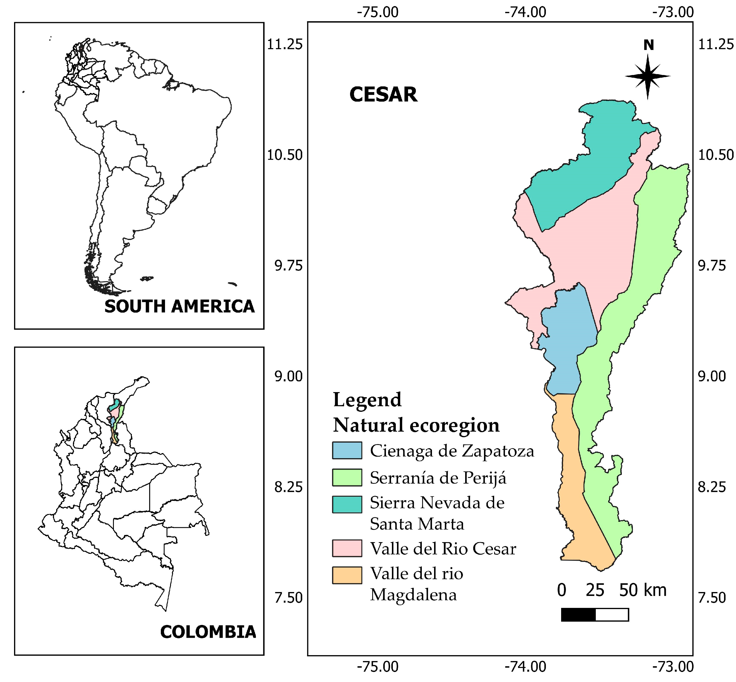
The Department of Cesar (CD) is a political and administrative territorial unit located on the Caribbean coast of Colombia, in northern South America, between latitudes 07°41′16″ N and 10°52′14″ N, and longitudes 72°53′27″ W and 74°08′28″ W, covering approximately 22,905 km2 (Figure 1). CD is an important agricultural, livestock, and agro-industrial center in the country. The natural subsystem presents a mountainous topography in 43% of the territory (elevation between 300 and 5600 masl) and plains in 57% (elevation below 100 masl) of the territory. The CD is divided into five natural ecoregions: the Sierra Nevada de Santa Marta to the northwest; the Serranía del Perijá, which runs through the entire department in its eastern zone; the Ciénaga de Zapatoza covering 300 km2 located in the center of the territory; the Valle del Río Cesar, which occupies the central part of the department and part of the Caribbean Plain; and the Valle del Río Magdalena in the southern part of the department, consisting of low, flat areas covered by dense forests. The Magdalena and Cesar Rivers, along with their tributaries, form the hydrographic network of the department. The climate of the CD is classified according to the Köppen-Geiger classification as Aw and Am [34]. This classification indicates that the region experiences a tropical savanna climate (Aw) and a tropical monsoon climate (Am). The Aw climate is characterized by distinct wet and dry seasons, with the dry season lasting for several months. On the other hand, the Am climate is characterized by a longer wet season, with significant rainfall throughout the year. The inclusion of these climate classifications in our study is important as it helps to provide a comprehensive understanding of the climatic conditions in the CD.
The annual precipitation ranges from 1000 to 1500 mm and the average annual temperature ranges from 24 to 35 °C [35]. The CD experiences a pluviometric climatic regime with three seasons [36]: dry (December–March), transitional (also known as the San Juan Summer) (June–July), and rainy (April–June and August–November).
Maize is the primary cereal crop in CD and is cultivated annually in two distinct seasons. The first sowing period occurs from late March to April, while the second sowing period occurs from the third week of August to the third week of September. It is essential to highlight that the average duration of the maize crop cycle in this region is around 120 days, encompassing different stages of growth and development until the final harvest is conducted. In 2022, 14,430 ha of maize were sown in Period I, followed by 17,790 ha in Period II [10]. The conventional farming approach yielded 2.41 tonnes per hectare of yellow maize during Period I, while the technified farming system achieved 5.25 tonnes per hectare. During Period II, the yield of yellow maize was 1.95 tonnes per hectare for the conventional scheme and 4.65 tonnes per hectare for the technified scheme.
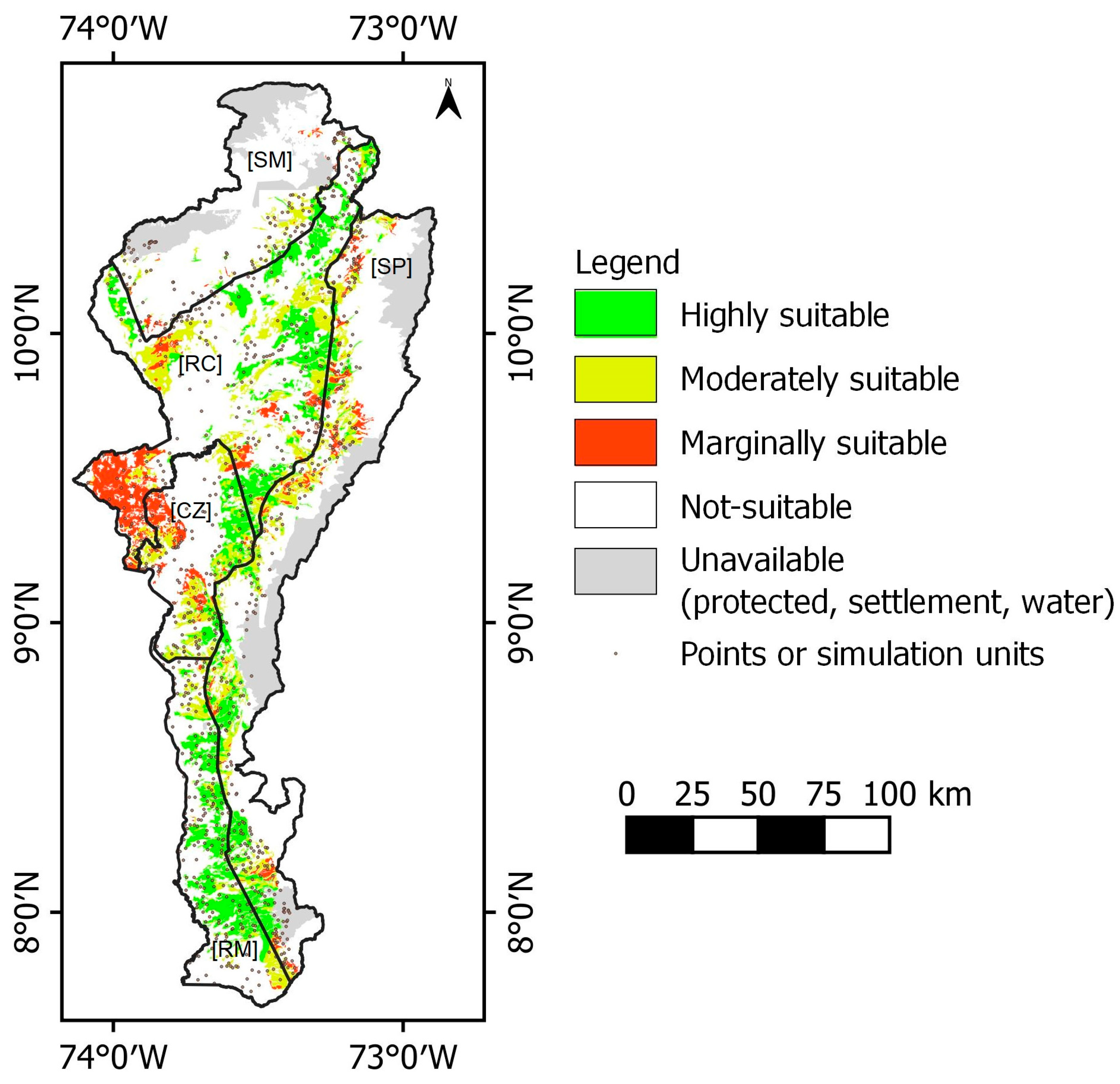
The suitability of the areas for maize farming in CD is shown in Figure 2, which indicates that only 27% of the total area of the region (619,689 ha) is appropriate for this crop. This area can be further classified into highly suitable (275,048 ha), moderately suitable (231,454 ha), marginally suitable (113,187 ha), and permanently unsuitable (1,355,290 ha) areas. In addition, 281,571 ha cannot be used for maize farming because they are designated as protected, settlement, or water areas [37]. It is interesting to note that although there are numerous suitable areas, maize is cultivated in just 5.2% of the potentially suitable areas for this crop in CD.

2.2. Classification of Precipitation Year-Types

When assessing the risks associated with maize planting, it is essential to consider three possible scenarios. The first scenario occurs when the water requirements of the current season are similar to those of an average year, resulting in an intermediate-year classification. The second scenario occurs when the water requirements of the current season exceed those of an average year, leading to a dry-year classification. In this case, early water consumption may cause a significant reduction in yield due to a water deficit. The third scenario occurs when the water requirements of the current season are lower than those of an average year, resulting in a wet-year classification.
A typical meteorological year methodology adjusted for the crop growth cycle of maize was used [20,21,22]. To achieve this, we determined the distribution of wet, intermediate, and dry years during the crop growth cycle within the framework of a 42-year series (1980–2022) for 60 meteorological stations distributed in the study area. The parameters used were daily reference evapotranspiration and precipitation because of their importance for irrigation requirements, as well as minimum and maximum daily temperatures because of their effects on ET0 and the phenological development of the crop. A precipitation deficit index (PD) (mm) was used to determine if a year was dry, intermediate, or wet (Equation (1)) [21].
P D = P E T 0
where PD is the precipitation deficit index, P is the accumulated precipitation, and ET0 is the evapotranspiration reference.
Based on the methodology proposed by Leite et al. [21], these 42 years were arranged from the highest to lowest standardized PD (Z) (Equation (2)).
Z = P D P D a v D S
where PDave is the average PD value of the series and DS is the standard deviation.
The data were statistically analyzed to assess whether they conformed to a normal distribution and were subsequently partitioned into three distinct groups (i.e., dry, intermediate, and wet years) with equal ranges (Equation (3)). This enabled the series of years to be classified into three broad categories (Equations (4)–(6)) based on their respective moisture levels and facilitated the generation of a typical meteorological year (TMY) that accurately represented each group.
R = Z m a x Z m i n N °   g r o u p s
D r y   Y e a r s = Z m i n Z Z m i n + R
I n t e r m e d i a t e   Y e a r s = Z m i n + R Z Z m a x R
W e t   Y e a r s = Z m a x R Z Z m a x
Following the methodology proposed by Dominguez et al. [20], constructing the Typical Meteorological Years (TMY) for the intermediate, dry, and wet scenarios involved a rigorous selection of individual months that accurately represented the characteristic climatic conditions of each identified group of years. Based on the classification of years within each scenario, we created a TMY for dry years, another for intermediate years, and an additional one for wet years. This process was implemented at the spatial level in the Department of Cesar using the Python programming language.
To conduct our simulations, we utilized daily data from the constructed TMYs. These typical years served as inputs for running simulations in the Aquacrop-OS model. Aquacrop-OS is a widely used crop simulation model that allows us to assess and analyze the potential yield of maize under different climatic conditions. By utilizing the TMY data, we were able to simulate and evaluate the maize yield response to varying weather patterns represented by the different TMY scenarios. This approach provides valuable insights into the crop’s performance and assists in agricultural planning and management decisions.
Dry and wet years can be considered risk factors for agriculture. In dry years, there is a risk of drought, which can significantly affect the crop yield and agricultural productivity. Similarly, in wet years, there is a risk of excessive precipitation, which can cause flooding and damage to crops. Farmers and agricultural professionals often view dry and wet years as risk levels that must be managed and mitigated to ensure optimal crop growth and yield.

2.3. AquaCrop Model

AquaCrop is a crop growth simulation model created by the Food and Agriculture Organization of the United Nations (FAO) and is intended to assess the water productivity of crops under varying environmental and management conditions [31]. The AquaCrop model conceptually simulates crop development by using four consecutive processes: canopy development, crop transpiration, biomass accumulation, and yield formation. The model simulates canopy development using canopy cover instead of the leaf area index (LAI). The central assumption of AquaCrop is that the accumulation of dry matter (B) is determined by crop transpiration (Tr) (Equations (7) and (8)).
W P * = f B T r E T 0 ,   C a
B = W P * B T r E T 0 ,   C a
where WP* represents normalized water productivity, B represents biomass, Tr represents crop transpiration, ET0 represents the reference evapotranspiration, and Ca represents the concentration of CO2 in the air.
The crop yield can be calculated as indicated in Equation (9):
Y = f H I   H I 0   B
where HI0 is the reference harvest index (HI) related to crop variety and phenology, and fHI denotes the stress adjustment factor (e.g., soil moisture and temperature stress).
The AquaCrop model requires the following input data: meteorological data (i.e., daily values of minimum/maximum temperature, precipitation, and reference evapotranspiration); soil parameters (i.e., soil texture, water content at saturation, field capacity, permanent wilting point, and hydraulic conductivity); crop type (i.e., parameters describing crop development and growth, including heat units and/or growing degree days for crop development, canopy cover, and root depth); and management strategies (i.e., planting date, fertilization, and irrigation, including frequency and amount of water applied). The model outputs were associated with crop canopy development and yield responses to water, biomass production, and soil water content during the growing season.
Previous studies have demonstrated the capability of the AquaCrop model to simulate maize yield and water-use efficiency in semi-arid environment [38,39,40]. Additionally, AquaCrop was used to estimate the spatial variability in maize yield and identify regions with high potential for maize production. Furthermore, AquaCrop is considered a useful tool for water allocation decisions and for identifying adaptation strategies that help minimize the negative effects of climate change on maize yield. In 2022, version 7.0 of the AquaCrop model was released, which is available for major operating systems such as Windows, Linux, and Mac OS. AquaCrop has been implemented in open-source code in Matlab/Octave, where it is known as AquaCrop-OS [41], AquaCropR [42], and AquaCrop-OSPy (ACOSP) [43].

2.4. Data

To simulate the growth of maize crops at a spatial level, the study area was divided into 1009 simulation units derived from the General Study of Soils and Land Zoning of the Department of Cesar, which was conducted in 2014 at a scale of 1:100,000 by the Instituto Geográfico Agustín Codazzí (IGAC) [44]. In Colombia, the IGAC maintains databases that are part of a national soil information service called the SIGA SIG. This service provides mapping information on soil mapping units and their corresponding profiles at a scale of 1:100,000. The types and sources of data required for this study are as follows.

2.4.1. Climate Data

This study employed a robust methodology for collecting and analyzing agroclimatology data in the Department of Cesar, Colombia. The data acquisition process involved utilizing a network of weather stations covering the five ecoregions provided by the Institute of Hydrology, Meteorology, and Environmental Studies (IDEAM). Quality control and filling procedures were applied to the daily temperature and precipitation data from 1980 to 2022, following the method proposed by Terán-Chaves et al. [45]. We incorporated 60 spatial points of supplementary data from the NASA LaRC POWER [46] (Prediction of Worldwide Energy Resource) database to enhance the climatological information. This dataset provides satellite-derived meteorological information at a spatial resolution of 0.5°. These datasets encompassed the period from 1980 to 2022 and included daily measurements of relative humidity, rainfall, solar radiation, wind speed, and direction. Reference evapotranspiration (ET0) was calculated using the FAO-56 Penman-Monteith method [47].

2.4.2. Soil Hydrological Parameters

A classical digital soil mapping approach was applied to map the soil properties required as inputs for the AquaCrop-OS model. This approach involved constructing a prediction function produced by an inverse distance weighting (IDW) geostatistical algorithm using ArcGIS 9.3. The spatial data used to predict the soil properties were obtained from the General Study of Soils of the Department of Cesar at a scale of 1:100,000 [44]. The obtained soil parameters included volumetric water content (m3 m−3), water content at field capacity (m3 m−3), water content at the permanent wilting point (m3 m−3), saturated hydraulic conductivity (mm day−1), soil texture (percentage of sand and clay), organic matter content (%), and density factor (dimensionless).
Figure 3 shows the soil texture patterns observed in the study area. The data revealed that clay was the most prevalent soil texture across all ecoregions, ranging from 29% to 49%. Sandy loam ranked as the second most abundant soil texture in the four ecoregions, accounting for 12% to 33% of the soil composition. However, it was absent in the Valle del Rio Magdalena [RM] ecoregion. Sandy clay loam covers a range of 1% to 24% and is more abundant in the Sierra Nevada de Santa Marta [SM] ecoregion. Loam covers a range of 10% to 23%, with the highest percentage found in the Valle del Rio Magdalena [RM] ecoregion. Clay loam ranged from 0% to 11%, with the highest percentage observed in the Serranía del Perijá [SP] ecoregion. Silty clay loam ranged from 0% to 5%, with the highest percentage found in the Valle del Rio Cesar [RC] ecoregion. The percentage of silty clay ranged from 0 to 9%, with the highest percentage found in the Valle del Rio Magdalena [RM] and Ciénaga de Zapatosa [CZ] ecoregions. Finally, loamy sand ranges from 0% to 4%, with the highest percentage observed in the Ciénaga de Zapatosa [CZ] ecoregion.

2.4.3. Crop Parameters

The AquaCrop-OS model requires 67 crop parameters obtained from validation experiments of the AquaCrop model for maize at a site scale conducted in 2022 at the Motilonia Research Center of the Colombian Corporation for Agricultural Research, located in the Department of Cesar, Colombia (10°2′ N, 73°16′ W, 339 m above sea level elevation). The yellow maize hybrid material Pioneer 30F-35, which is widely used in this region, was used for the field experiments. After adjusting the crop parameters to local conditions, a regional estimation of productivity was conducted using available historical information on maize cultivation in the Department of Cesar [10]. Details of the crop parameters are presented in the Supplementary Material (Table S1).
To capture the effect of changes in rainfall patterns, we simulated the achievable maize yield under three types of precipitation years (dry year, TMY, and wet year) and two different water-use strategies (irrigated and precipitation). Fixed planting dates were considered for period I (March 25th of each reference year) and Period II (August 20th of each reference year).
In this study, the open-source version of AquaCrop-OS was used. Owing to the geospatial framework of the simulations, the ‘AquaCropOS_BatchRUN.m’ script was executed in parallel using the Parallel Computing Toolbox in MATLAB. We defined 1009 (simulation units) separate sets of input files for each simulation run, and the batch simulation was executed in parallel.

2.5. Derivation of the Vulnerability Curves

Vulnerability curves in the form of logistic S-shaped curves were developed specifically for two typical maize planting periods, adapted to the context of the Cesar Department. Vulnerability curves were constructed by considering the biophysical characteristics of the five ecoregions with different soil textures.
Vulnerability curves were constructed based on the relationship between the intensity of water stress and yield loss rate [24,25,26,48]. In the metric of the vulnerability curve, the y-axis is typically represented by a fraction of the loss or damage component (0–100%), and the x-axis is represented by the crop water stress index. To generate vulnerability curves for maize using AquaCrop-OS, the model was executed with different levels of soil water availability, in two planting periods over three specific years according to local precipitation regimes (dry year, TMY, and wet year) and two water management practices (100% irrigation and rainfed), while keeping other environmental conditions constant (e.g., temperature, solar radiation, and soil properties). This information can be used to optimize irrigation management and guide the development of sustainable agricultural policies. Finally, we adjusted the vulnerability curves to express the relationship between yield loss rate and drought intensity. Based on previous studies, we used a logistic vulnerability curve [24,25,26,48].
Using the AquaCrop-OS model, we simulated maize crop yields at a spatial level in the study area, considering the different climatic conditions of three specific years and two water management approaches (irrigation and rainfed). We used Equation (10) to estimate the yield loss rate (YLR) [26].
Y L R = 1 Y 2 Y 1 × 100 %
where YLR is the yield loss rate and Y1 and Y2 represent the maize yields (per unit) in the 100% irrigation scenario and other scenarios, respectively.
The crop water stress indicator (CWSI) was employed as a tool to determine the severity of water stress. The CWSI gauges water stress by measuring the deviation between actual and potential evapotranspiration (Equation (11)). Its value ranges between zero and one, with a higher CWSI indicating more intense water stress. Wu et al. [33] classified the severity of the CWSI into four categories: a CWSI score of 0–0.25 is classified as slight drought, 0.25–0.5 as moderate drought, 0.5–0.75 as severe drought, and 0.75–1 as extreme drought.
C W S I = 1 T r c E T 0
where Trc and ET0 represent the actual transpiration of the crop and reference evapotranspiration (mm), respectively. Both Trc and ET0 were the results of the AquaCrop model computed on a daily scale.
To account for the accumulated impact of water stress over time, the drought hazard index (DHI) was established as the average daily value of CWSI throughout the growing season. This can be expressed mathematically as shown in Equation (12):
D H I = 1 n   i = 1 n C W S I i
where DHI represents the drought hazard index, CWSIi is the crop water stress index on the ith day, and n is the number of days in the growth season.

3. Results

3.1. Determination of Dry, Intermediate, and Wet Years

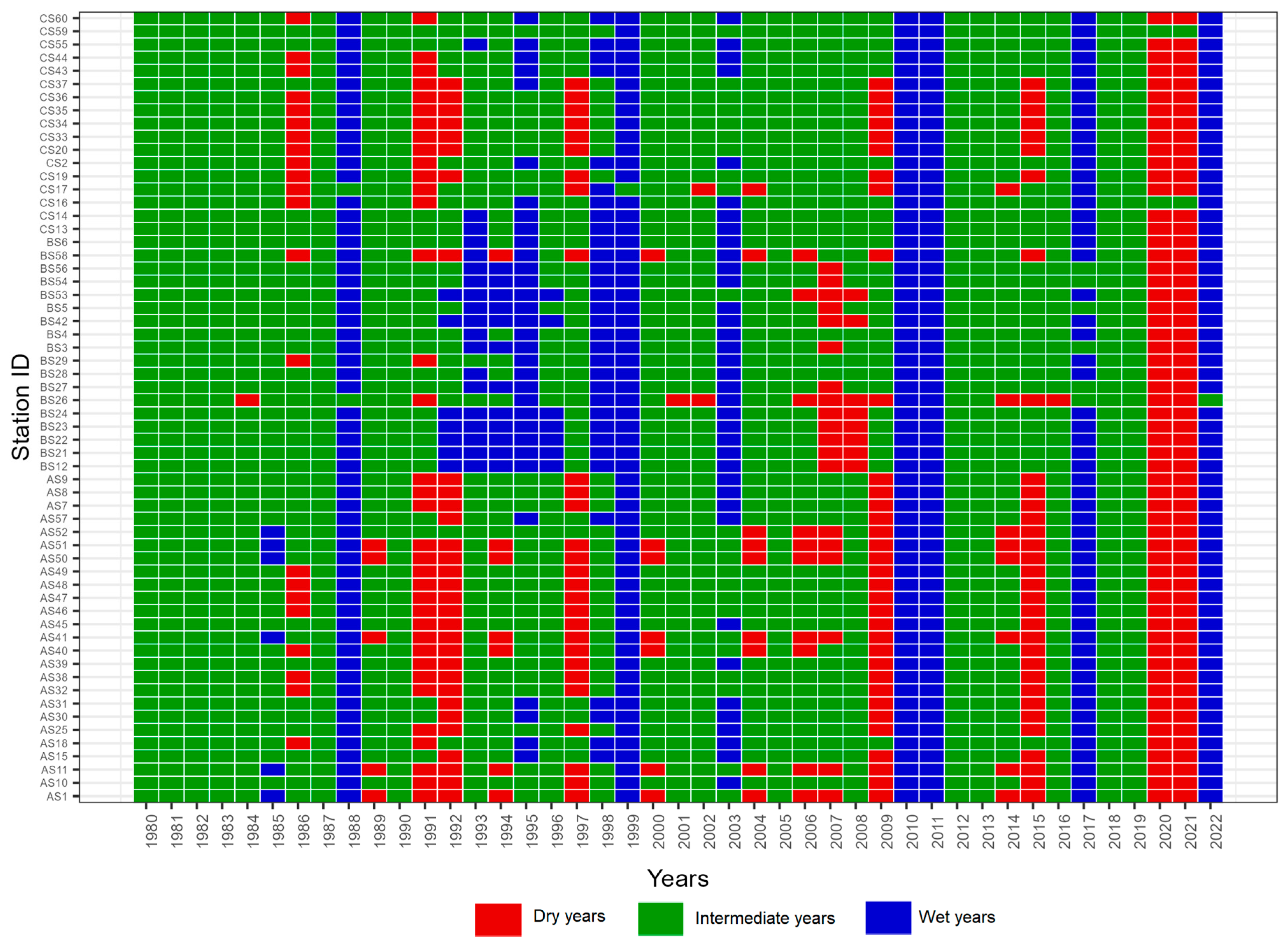
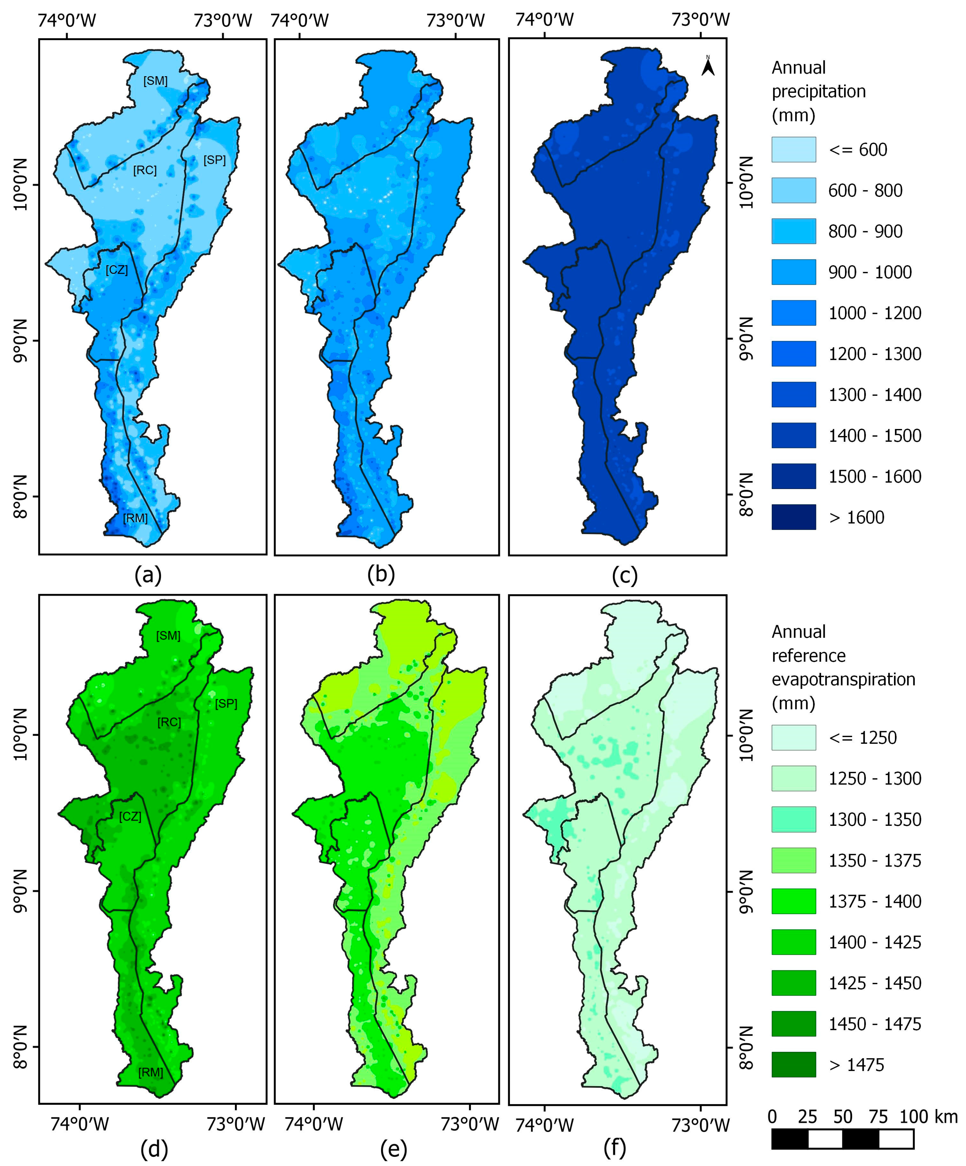
The results revealed that 66.6% of the years in the region could be classified as intermediate, whereas wet years occurred more frequently (19.5%) than did dry years (14.7%). These events demonstrated a regular pattern of wet years, occurring once every 11 years at most of the stations. Conversely, dry years recurred every 5–11 years, but their spatial distribution was less widespread in the region (Figure 4). To further investigate these climatic patterns, typical meteorological years were identified for each category, based on the years from each group. In this regard, Figure 5 shows the precipitation and reference evapotranspiration data for each of the Typical Meteorological Years (TMYs) calculated under dry, intermediate, and wet conditions. The graph provides a visual representation of the climatic characteristics of these TMY scenarios, showcasing the variation in precipitation and evapotranspiration patterns.

3.2. AquaCrop Model Validation

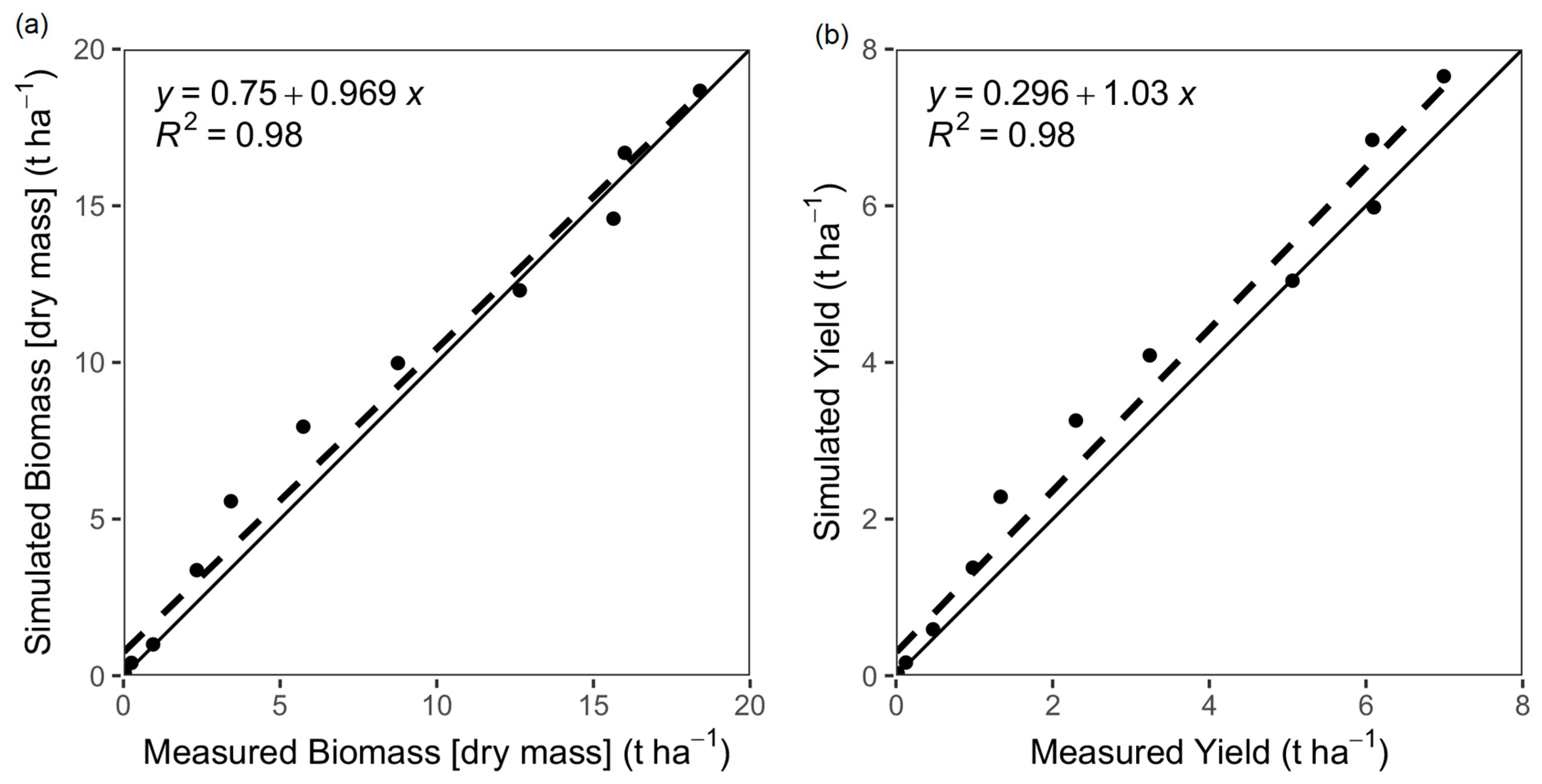
The measured grain yields in the field experiments ranged from 1.0 ± 0.7 to 2.2 ± 0.7 t ha−1 under rainfed conditions and from 4.4 ± 1.3 to 8.0 ± 0.8 t ha−1 under optimal irrigation conditions. The reduction in maize grain yield occurs primarily when maize experiences stress during the reproductive growth stage [49]. The AquaCrop model was validated to simulate grain yield using experimental data obtained during the 2022 season, and the results are presented in Figure 6. To assess the performance of the model, statistical parameters were used, such as the normalized root mean square error (NRMSE), Nash–Sutcliffe model efficiency coefficient (EF), and Willmott’s index of agreement (d). The results indicated a strong agreement between the measured and simulated grain yields, with an R2 value of 0.98 and an EF value of 0.91, both of which are within acceptable limits. The validation process yielded an RMSE value of 1.08 and a d value of 0.99, suggesting that the grain yield predicted by the model under validation was similar to that measured under both rainfed and irrigated conditions.
Validation of the AquaCrop model revealed that the model’s simulated maize grain values were consistent with the measured data, even under rainfed conditions. However, the highest prediction error for grain yield was obtained for the rain-fed treatments (30.47%). This discrepancy is because water stress significantly reduced grain yield during the experiment. Furthermore, the model overestimated grain yield in the rainfed treatment, resulting in a higher prediction error. Figure 6 shows that the simulated yield values were relatively close to the 1:1 line compared with the measured yield values.

3.3. Vulnerability Assessment

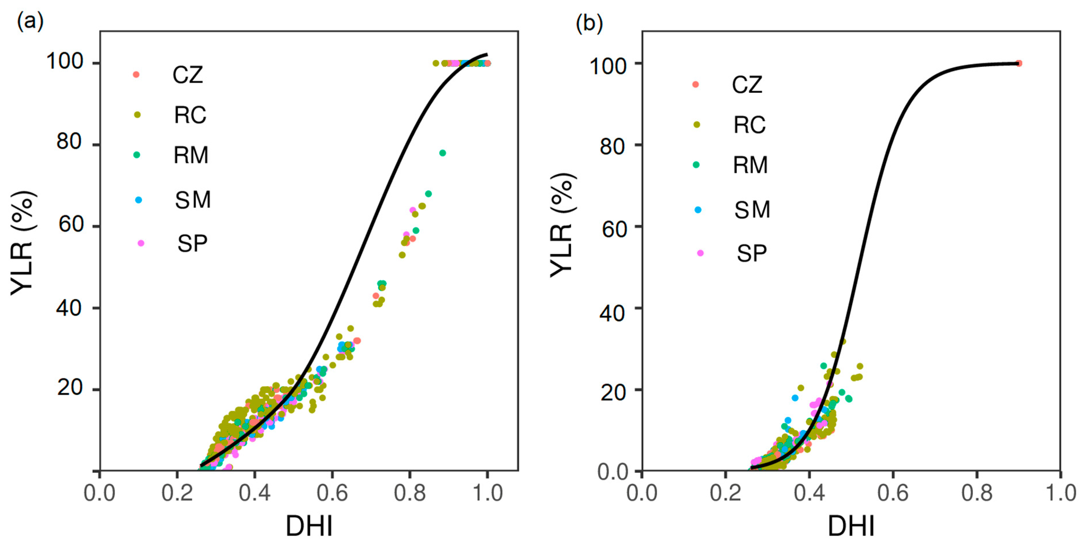
Figure 7 illustrates the vulnerability curves for the complete maize growth season during period I and period II, which exhibit a characteristic “S” shape. The data points used in the curves were generated from simulations of maize growth in five distinct ecoregions in the Department of Cesar. The coefficients of determination (R2) for periods I and II were 0.93 and 0.91, respectively, indicating that the logistic curve provides a suitable representation of the relationship between DHI and YLR. For period I (Figure 7a), the vulnerability curve showed that the rate of increase in yield loss ratio (YLR) increased when DHI was between 0.5 and 0.8, and finally returned to being slow when DHI was above 0.9. It should be noted that out of the 1009 simulation units, 58% had a 100% yield loss, with a DHI of 0.9 or higher. However, for period II, the maize crop exhibited a lower degree of vulnerability (Figure 7b), with the range of the yield loss rate for 64% of the simulation units falling between 5% and 30%. For the remaining 36% of the simulated units, once the DHI of 0.9 was reached, the increase in the rate of yield loss was attenuated until it reached 100%.

3.3.1. Crop Water Stress Indicator

Figure 8 shows the values of the water stress indicator for maize cultivation that can be expected in a dry year, typical meteorological year (TMY), and wet year for the two representative planting periods in the study area. The environmental conditions for maize cultivation in period II favored the crop in the study area compared with the conditions in period I (Figures S1 and S2), as reflected in the lower crop water stress indices (on average 20% lower) and, consequently, lower grain yield losses. Overall, under the TMY scenario, maize cultivation in the department of Cesar experienced severe drought conditions (0.5 < DHI < 0.75) in periods I (DHI = 0.68) and II (DHI = 0.51). In a dry year, the severity of drought was extreme in period I and severe in period II, whereas in a wet year, the water stress of maize cultivation was moderate in both planting periods. In period I, the Sierra Nevada De Santa Marta [SM] ecoregion experienced the most severe drought intensity across all three precipitation year types, with average DHI values of 0.90, 0.75, and 0.57 in the dry year, TMY, and wet year, respectively. The Serranía del Perijá [SP] ecoregion was followed by an average DHI of 0.88, 0.76, and 0.54 in the dry, TMY, and wet years, respectively. In contrast, the Ciénaga De Zapatosa [CZ] and Valle Del Rio Magdalena [RM] ecoregions presented moderate to severe drought risks (Table 1).

3.3.2. Risk of Yield Loss (YLR)

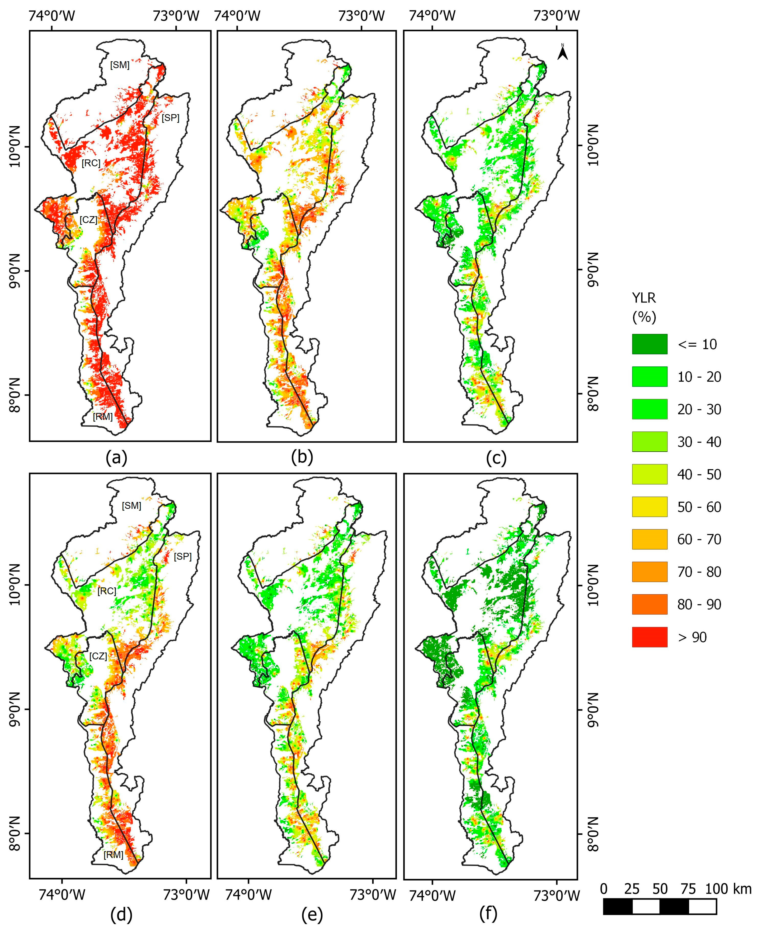
The rate of maize yield loss was calculated for the three years during the two planting periods, according to the regional crop calendar (periods I and II). On average, the yield losses were lower in period II (Table 2). In dry years, YLR values ranged from a minimum of 34.33% in the Valle Del Rio Cesar [RC] during Period II to a maximum of 100% in the Sierra Nevada De Santa Marta [SM] during period I. This indicates that, in dry years, the ecoregions experienced more severe maize grain yield losses. In wet years, the YLR values were generally lower than in dry years, with values ranging from a minimum of 8.25% in the Sierra Nevada De Santa Marta [SM] during period I to a maximum of 39.74% in the Valle Del Rio Magdalena [RM] during period II. The risk of maize yield loss increased from south to north, which is in line with the DHI distribution trend (Figure 9).
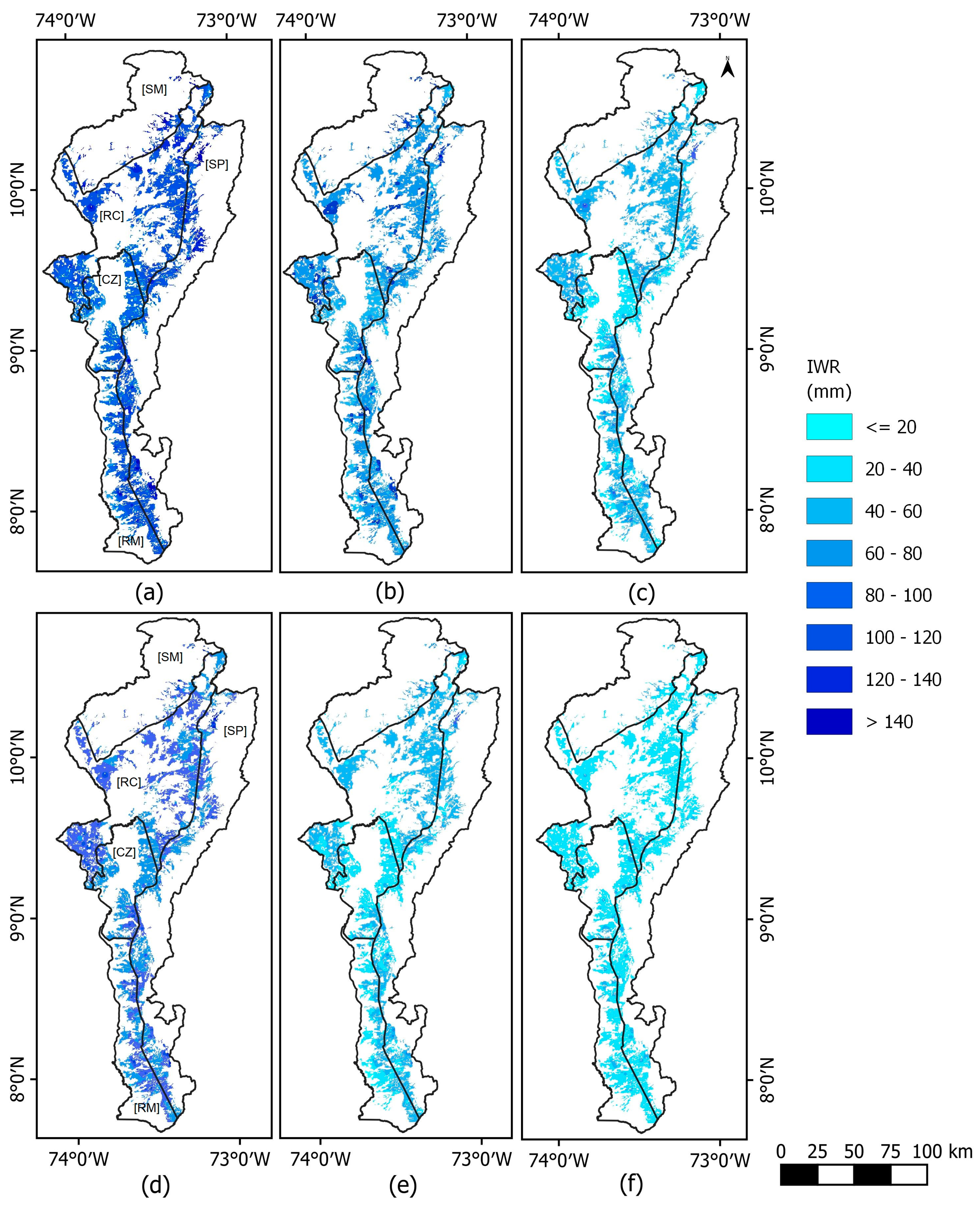
The study found that maintaining acceptable levels of maize production in period I largely depended on irrigation, whereas in period II, rainfall satisfied most of the crop’s water demand. The irrigation water requirement (IWR) was estimated using the AquaCrop-OS model, and the values of IWR represent the total amount of irrigation water (in millimeters) required to meet the crop water demands during the growing period (Figure 10). The results showed that in the dry year scenario, IWR values are relatively high, ranging from 136.3 mm in the Sierra Nevada de Santa Marta [SM] ecoregion to 66.2 mm in the Ciénaga de Zapatosa [CZ] region for period-I and from 94.9 mm to 71.3 mm for period-II. These high values indicate that crop water requirements are particularly high during dry years, which can be attributed to the lower precipitation levels and higher evapotranspiration rates. For the TMY scenario, IWR values were generally lower than those in the dry year scenario but higher than those in the wet year scenario, reflecting the average water demand of maize crops in Cesar under typical climatic conditions.
The IWR values for the TMY scenario range from 84.5 mm in the Sierra Nevada de Santa Marta [SM] ecoregion to 32.7 mm in the Valle del Río Magdalena [RM] ecoregion for period-I and from 57.4 mm to 35.6 mm for period-II. In the wet year scenario, IWR values are the lowest among the three types of years, ranging from 58.2 mm in the Sierra Nevada de Santa Marta [SM] region to 31.2 mm in the Ciénaga de Zapatosa [CZ] region for period-I and from 39.4 mm to 32.7 mm for period-II. This could be attributed to the higher precipitation levels and lower evapotranspiration rates during wet years, resulting in a lower need for additional irrigation water.
Overall, these IWR values provide useful information for farmers in the area, allowing them to estimate the amount of water needed to meet their crops’ water demands under different climatic conditions, and to design more efficient and sustainable irrigation systems.

4. Discussion

In our study, we observed that under rainfed conditions during the dry year, the maize crop growth period ended earlier than expected due to severe water stress in 87% of the study area in period I and 56% in period II. Similarly, during the typical meteorological year (TMY), the growth period ended earlier than expected in 58% and 35% of the area during periods I and II, respectively. However, in the wet year, the majority of maize crop simulations were able to complete the growth cycle, with only 25% and 17% of the area ending earlier than expected. These results indicate the high sensitivity of maize in the Cesar department to drought conditions and its strong response in the early stages of the crop [24,26,31].
Previous studies have shown that maize is particularly sensitive to water deficits during the flowering stage [24,26,31]. Monteleone et al. [24] reported significant yield losses under water stress during the flowering stage, especially in loamy soils. In our study, the severe to extreme water stress experienced in period I, which coincided with the crop’s phenology during the flowering stage, likely contributed to higher grain yield losses compared to period II. To adapt and mitigate grain losses, it is crucial to consider adjusting the typical planting calendar for the region to avoid the water scarcity period, especially in dry scenarios when available resources may be insufficient to meet the required irrigation water demand.
Crops under drought stress often exhibit enhanced water use efficiency as an adaptive response to sub-optimal environmental conditions [50]. This phenomenon was observed in the department of Cesar with maize, which achieved an average water productivity of 1.41 kg m−3 during the drought scenario. In contrast, during the wet year, the water productivity of maize was only 1.19 kg m−3. Calculating the respective water footprints in these two scenarios yielded values of 0.711 m3 kg−1 and 0.842 m3 kg−1, respectively.
Furthermore, our study revealed that different soil types exhibited varying responses in terms of yield loss ratio (YLR) under different environmental conditions. Loam, sandy loam, and sandy clay loam soils generally displayed relatively high YLR under dry, normal, and wet conditions, whereas clay soils tended to have lower YLR responses. It is important to note that crop yields are influenced by various factors, including nutrient content and management practices, in addition to soil type. Moreover, the hydraulic conductivity of clay soils was found to be lower compared to other soil types in the study area. This characteristic enhances the water holding capacity at the microscopic level, ensuring water availability for plant roots over extended periods, particularly during drought or water stress. This property contributes to increased water supply to the root zone, enabling plants to withstand prolonged water stress and enhance their resilience [24,51].
Overall, our findings emphasize the vulnerability of maize to water stress, particularly during the flowering stage, and highlight the importance of implementing adaptive measures in agricultural practices to mitigate yield losses. Understanding the interactions between crop response, soil characteristics, and environmental conditions provides valuable insights for enhancing crop management strategies and promoting sustainable agriculture in water-limited regions.

5. Conclusions

In this study, we quantified the vulnerability and risk of maize cultivation in five ecoregions of the Cesar Department, a semi-arid region in northern Colombia (South America), using a multistep process to model crop water stress indices, crop vulnerability curves, and crop yield under three scenarios based on precipitation anomalies.
Vulnerability encompasses both physical and social aspects that may not be separable. This study mainly focused on physical vulnerability and did not consider socioeconomic factors that may impact vulnerability. Such factors fall outside the scope of this study and will be examined later. For future investigations, these biophysical results can be related to the socioeconomic conditions of maize-producing areas, which will help improve these results and find elements that are more in line with the local realities and production limitations faced by producers.
The regional decision-making process for the planting date of period I can be optimized to avoid maize grain production losses. For instance, in TMY, which represents the most frequent environmental condition, potential losses of 64.4% in production are generated. The irrigation requirements were consistent under dry, TMY, and wet-year conditions. These results demonstrate that the use of TMY to determine the irrigation depth for maize cultivation in the five ecoregions can allow farmers to achieve adequate yields, avoid high water deficits, and make efficient use of available water in the Cesar Department.
The importance of this study lies in its contribution to our understanding of the response of maize cultivation to different precipitation regimes at the regional level. The results provide valuable information for farmers and policymakers regarding areas that are suitable for maize cultivation and the potential yield under different climatic conditions. Additionally, vulnerability curves and risk distribution can help farmers and policymakers develop effective strategies to minimize the negative impacts of climate variability on maize crop yield, ultimately contributing to food security and sustainable agricultural practices. This study emphasizes the significance of employing models such as AquaCrop-OS for simulating crop yields under diverse climatic conditions and within extensive geospatial frameworks. Such models play a crucial role in informing decision-making processes pertaining to agricultural management.
Supplementary Materials

The following supporting information can be downloaded at: https://www.mdpi.com/article/10.3390/w15112108/s1: Table S1. Input data of crop parameters used in AquaCrop-OS model; Figure S1. Spatial distribution of yield (t ha−1) of maize in different precipitation year types at the Department of Cesar. (a) yield in dry year period-I rainfed, (b) yield in TMY period-I rainfed, (c) yield in wet year period-I rainfed, (d) yield in dry year period-I irrigation 100%, (e) yield in TMY period-I irrigation 100%, and (f) yield in wet year period-I irrigation 100%. Yield was simulated by the AquaCrop-OS model; Figure S2. Spatial distribution of yield (t ha−1) of maize in different precipitation year types at the Department of Cesar. (a) Yield in dry year period-II rainfed, (b) yield in TMY period-II rainfed, (c) yield wet year period-II rainfed, (d) yield in dry year period-II irrigation 100%, (e) yield in TMY period-II irrigation 100%, and (f) yield in wet year period-II irrigation 100%. Yield was simulated by the AquaCrop-OS model.

Author Contributions

Conceptualization, C.A.T.-C. and S.M.P.-M.; data curation, C.A.T.-C. and S.M.P.-M. and A.V.-A. software, and C.A.T.-C. and J.M.D.-C.; formal analysis, C.A.T.-C. and S.M.P.-M.; investigation: C.A.T.-C. and S.M.P.-M.; methodology, C.A.T.-C.; resources, C.A.T.-C.; supervision, C.A.T.-C. and S.M.P.-M.; visualization, C.I.-C. and S.M.P.-M.; writing—original draft, S.M.P.-M. and C.A.T.-C. Writing—review and editing: S.M.P.-M. All authors have read and agreed to the published version of the manuscript.

Funding

This paper was developed within the framework of the project “Optimización del agua y uso eficiente del suelo para mejorar la producción agropecuaria en escenarios de vulnerabilidad agroclimática del departamento del Cesar”—BPIN 2017000100050—supported by the Colombian Fund for Science, Technology, and Innovation of General System Royalties (FCTeI-SGR), together with Gobernación del Cesar funds.

Data Availability Statement

Not applicable.

Acknowledgments

The authors express their gratitude to all the Centro de Investigación Motilonia-AGROSAVIA (Cesar, Colombia) staff for logistical and instrumental support provided during the practical development of this work. Likewise, the authors thank the Secretaría de Agricultura y Desarrollo Empresarial of Cesar Department and Prodesarrollo Ltda. We also thank the anonymous reviewers for their valuable and constructive comments.

Conflicts of Interest

The authors declare no conflict of interest.

References

  1. Food and Agriculture Organization of the United Nations. FAOSTAT Statistical Database. Rome. 2022. Available online: https://www.fao.org/faostat/en/ (accessed on 2 January 2023).
  2. Ray, D.K.; Gerber, J.S.; Macdonald, G.J.; West, P.C. Climate variation explains a third of global crop yield variability. Nat. Commun. 2015, 6, 5989. [Google Scholar] [CrossRef] [PubMed] [Green Version]
  3. Bouroncle, C.; Müller, A.C.; Giraldo, D.L.; Ríos, D.; Imbach, P.; Girón, E.; Portillo, F.; Boni, A.; Van Etten, J.; Ramirez-Villegas, J. A systematic approach to assess climate information products applied to agriculture and food security in Guatemala and Colombia. Clim. Serv. 2019, 16, 100137. [Google Scholar] [CrossRef]
  4. Kerr, R.B.; Naess, L.O.; Allen-O’Neil, B.; Totin, E.; Nyantakyi-Frimpong, H.; Risvoll, C.; Rivera-Ferre, M.G.; López-I-Gelats, F.; Eriksen, S. Interplays between changing biophysical and social dynamics under climate change: Implications for limits to sustainable adaptation in food systems. Glob. Chang. Biol. 2022, 28, 3580–3604. [Google Scholar] [CrossRef] [PubMed]
  5. Pellegrina, H.S.; Gafaro, M. Trade, farmers’ heterogeneity, and agricultural productivity: Evidence from Colombia. J. Int. Econ. 2022, 137, 103598. [Google Scholar] [CrossRef]
  6. Jha, C.K.; Gupta, V. Farmer’s perception and factors determining the adaptation decisions to cope with climate change: An evidence from rural India. J. Environ. 2021, 10, 100112. [Google Scholar] [CrossRef]
  7. Guzzon, F.; Arandia Rios, L.W.; Caviedes Cepeda, G.M.; Céspedes Polo, M.; Chavez Cabrera, A.; Muriel Figueroa, J.; Medina Hoyos, A.E.; Jara Calvo, T.W.; Molnar, T.L.; Narro León, L.A.; et al. Conservation and Use of Latin American Maize Diversity: Pillar of Nutrition Security and Cultural Heritage of Humanity. Agronomy 2021, 11, 172. [Google Scholar] [CrossRef]
  8. Bouroncle, C.; Imbach, P.; Rodríguez-Sánchez, B.; Medellín, C.; Martinez-Valle, A.; Läderach, P. Mapping climate change adaptive capacity and vulnerability of smallholder agricultural livelihoods in Central America: Ranking and descriptive approaches to support adaptation strategies. Clim. Chang. 2017, 141, 123–137. [Google Scholar] [CrossRef] [Green Version]
  9. Howland, F. Local climate change policy and rural development in Colombia’s post-peace agreements context. Int. J. Agric. Sustain. 2022, 20, 1260–1277. [Google Scholar] [CrossRef]
  10. Federación Nacional de Cultivadores de Cereales, Leguminosas y Soya. Fenalce. Statistical Database. Bogotá. 2022. Available online: https://fenalce.co/estadisticas/ (accessed on 2 January 2023).
  11. CIMMYT. Maíz Para Colombia. Visión 2030. 2018. Available online: https://fenalce.co/wp-content/uploads/2021/10/Maiz-para-Colombia.pdf (accessed on 2 January 2023).
  12. United Nations Development Programme. The Sustainable Development Goals (SDGs). 2016. Available online: https://www.undp.org/sustainable-development-goals (accessed on 5 January 2023).
  13. Palacios-Rojas, N.; McCulley, L.; Kaeppler, M.; Titcomb, T.J.; Gunaratna, N.S.; Lopez-Ridaura, S.; Tanumihardjo, S.A. Mining maize diversity and improving its nutritional aspects within agro-food systems. CRFSFS 2020, 19, 1809–1834. [Google Scholar] [CrossRef]
  14. Ramirez-Villegas, J.; Salazar, M.H.; Jarvis, A.; Racines, C. A way forward on adaptation to climate change in Colombian agriculture: Perspectives towards 2050. Clim. Chang. 2012, 115, 611–628. [Google Scholar] [CrossRef]
  15. Monteleone, B.; Borzí, I.; Bonaccorso, B.; Martina, M. Quantifying crop vulnerability to weather-related extreme events and climate change through vulnerability curves. Nat. Hazards. 2016, 141, 123–137. [Google Scholar] [CrossRef]
  16. Vanuytrecht, E.; Raes, D.; Steduto, P.; Hsiao, T.C.; Fereres, E.; Heng, L.Y.; Vila, M.G.; Moreno, P.I. AquaCrop: FAO’s crop water productivity and yield response model. Env. Model Softw. 2014, 62, 351–360. [Google Scholar] [CrossRef]
  17. Corbeels, M.; Berre, D.; Rusinamhodzi, L.; Lopez-Ridaura, S. Can we use crop modelling for identifying climate change adaptation options? Agric. For. Meteorol. 2018, 256, 46–52. [Google Scholar] [CrossRef]
  18. Sinclair, T.R.; Soltani, A.; Marrou, H.; Ghanem, M.E.; Vadez, V. Geospatial assessment for crop physiological and management improvements with examples using the simple simulation model. Crop Sci. 2019, 60, 700–708. [Google Scholar] [CrossRef]
  19. Jha, P.C.; Araya, A.; Stewart, Z.P.; Faye, A.; Traore, H.; Middendorf, B.J.; Prasad, P.W.C. Projecting potential impact of COVID-19 on major cereal crops in Senegal and Burkina Faso using crop simulation models. Agric. Syst. 2021, 190, 103107. [Google Scholar] [CrossRef]
  20. Domínguez, A.; Martínez-Romero, A.; Leite, K.N.; Tarjuelo, J.M.; De Juan, J.; López-Urrea, R. Combination of typical meteorological year with regulated deficit irrigation to improve the profitability of garlic growing in central Spain. Agric. Water Manag. 2013, 130, 154–167. [Google Scholar] [CrossRef]
  21. Leite, K.N.; Martínez-Romero, A.; Tarjuelo, J.M.; Domínguez, A. Distribution of limited irrigation water based on optimized regulated deficit irrigation and typical metheorological year concepts. Agric. Water Manag. 2015, 148, 164–176. [Google Scholar] [CrossRef]
  22. Cano, A.; Pardo, J.J.; Montero, J.; Domínguez, A. Determining Irrigation Requirements of Extensive Crops Using the Typical Meteorological Year Adjusted to the Growing Cycle Period. Agronomy 2022, 12, 2208. [Google Scholar] [CrossRef]
  23. Gobin, A.; Van De Vyver, H. Spatio-temporal variability of dry and wet spells and their influence on crop yields. Agric. For. Meteorol. 2021, 308, 108565. [Google Scholar] [CrossRef]
  24. Monteleone, B.; Borzí, I.; Bonaccorso, B.; Martina, M.L.V. Developing stage-specific drought vulnerability curves for maize: The case study of the Po River basin. Agric. Water Manag. 2022, 269, 107713. [Google Scholar] [CrossRef]
  25. Li, F.; Manjing, Z.; Yaoze, L. Quantitative research on drought loss sensitivity of summer maize based on AquaCrop model. Nat. Hazards 2022, 112, 1065–1084. [Google Scholar] [CrossRef]
  26. Zhu, X.; Xu, K.; Liu, Y.; Guo, R.; Chen, L. Assessing the vulnerability and risk of maize to drought in China based on the AquaCrop model. Agric. Syst. 2021, 189, 103040. [Google Scholar] [CrossRef]
  27. Guo, H.; Wang, R.; Garfin, G.M.; Zhang, A.; Lin, D.; Qin’ou, L.; Wang, J. Rice drought risk assessment under climate change: Based on physical vulnerability a quantitative assessment method. Sci. Total Environ. 2021, 751, 141481. [Google Scholar] [CrossRef] [PubMed]
  28. Basso, B.; Liu, L.; Ritchie, J.T. A Comprehensive Review of the CERES-Wheat, -Maize and -Rice Models’ Performances. Adv. Agron. 2015, 136, 27–132. [Google Scholar] [CrossRef]
  29. Eggen, M.; Ozdogan, M.; Zaitchik, B.F.; Ademe, D.; Foltz, J.D.; Simane, B. Vulnerability of sorghum production to extreme, sub-seasonal weather under climate change. Environ. Res. Lett. 2019, 8, 045005. [Google Scholar] [CrossRef]
  30. Hendrawan, V.S.A.; Komori, D. Developing flood vulnerability curve for rice crop using remote sensing and hydrodynamic modeling. IJDRR 2021, 54, 102058. [Google Scholar] [CrossRef]
  31. Steduto, P.; Hsiao, T.C.; Raes, D.; Fereres, E. AquaCrop-The FAO Crop Model to Simulate Yield Response to Water: I. Concepts and Underlying Principles. Agron. J. 2009, 101, 426–437. [Google Scholar] [CrossRef] [Green Version]
  32. Wang, Z.; Wang, F.; Zhang, Y. Spatio-temporal Distribution Characteristics and Influencing Factors of Drought in Anhui Province Based on CWSI. J. Nat. Res. 2018, 33, 853–866. [Google Scholar]
  33. Wu, H.; Xiong, D.; Liu, B.; Zhang, S.; Yuan, Y.; Fang, Y.; Chidi, C.L.; Dahal, N.M. Spatio-Temporal Analysis of Drought Variability Using CWSI in the Koshi River Basin (KRB). Int. J. Environ. Res. Public Health 2019, 16, 3100. [Google Scholar] [CrossRef] [Green Version]
  34. Kottek, M.; Grieser, J.; Beck, C.; Rudolf, B.; Rubel, F. World Map of the Köppen-Geiger climate classification updated. Meteorol. Z. 2006, 15, 259–263. [Google Scholar] [CrossRef]
  35. Institute of Hydrology, Meteorology, and Environmental Studies. IDEAM. Atlas Climatológico de Colombia. Bogotá. 2018. Available online: http://atlas.ideam.gov.co/ (accessed on 26 January 2023).
  36. González-Álvarez, Á.; Viloria-Marimón, O.M.; Coronado-Hernández, O.E.; Vélez-Pereira, A.M.; Tesfagiorgis, K.; Coronado-Hernández, J.R. Isohyetal Maps of Daily Maximum Rainfall for Different Return Periods for the Colombian Caribbean Region. Water 2019, 11, 358. [Google Scholar] [CrossRef] [Green Version]
  37. Plan Departamental de Extensión Agropecuaria 2020-2023. PDEA Cesar. Departamento del Cesar. Valledupar, Colombia. 2020. Available online: https://www.minagricultura.gov.co/ministerio/direcciones/PublishingImages/Paginas/PDEA/PDEA%20CESAR%202020-%202023.pdf (accessed on 27 January 2023).
  38. Sandhu, R.; Irmak, S. Assessment of AquaCrop model in simulating maize canopy cover, soil-water, evapotranspiration, yield, and water productivity for different planting dates and densities under irrigated and rainfed conditions. Agric. Water Manag. 2019, 224, 105753. [Google Scholar] [CrossRef]
  39. Umesh, B.; Reddy, K.S.; Polisgowdar, B.S.; Maruthi, V.; Satishkumar, U.; Rao, S.A.; Veeresh, H. Assessment of climate change impact on maize (Zea mays L.) through aquacrop model in semi-arid alfisol of southern Telangana. Agric. Water Manag. 2022, 274, 107950. [Google Scholar] [CrossRef]
  40. Lu, Y.; Chibarabada, T.P.; Hoteit, I.; De Lannoy, G.; Sheffield, J. Global sensitivity analysis of crop yield and transpiration from the FAO-AquaCrop model for dryland environments. Field Crops Res. 2021, 269, 108182. [Google Scholar] [CrossRef]
  41. Foster, T.J.; Brozovic, N.; Butler, A.P.; Neale, C.M.U.; Raes, D.; Steduto, P.; Fereres, E.; Hsiao, T.C. AquaCrop-OS: An open source version of FAO’s crop water productivity model. Agric. Water Manag. 2017, 181, 18–22. [Google Scholar] [CrossRef]
  42. Camargo Rodriguez, A.V.; Ober, E.S. AquaCropR: Crop Growth Model for R. Agronomy 2019, 9, 378. [Google Scholar] [CrossRef] [Green Version]
  43. Kelly, T.D.; Foster, T. AquaCrop-OSPy: Bridging the gap between research and practice in crop-water modeling. Agric. Water Manag. 2021, 254, 106976. [Google Scholar] [CrossRef]
  44. Instituto Geográfico Agustín Codazzi. IGAC. Estudio General de Suelos y Zonificación de Tierras del Departamento de Cesar. Subdirección de Agrología. Bogotá 2014. Available online: https://geoportal.igac.gov.co/ (accessed on 4 February 2022).
  45. Terán-Chaves, C.A.; Duarte-Carvajalino, J.M.; Polo-Murcia, S. Quality control and filling of daily temperature and precipitation time series in Colombia. Meteorol. Z. 2021, 30, 489–501. [Google Scholar] [CrossRef]
  46. NASA Langley Research Center. Meteorological Data Sets from NASA. 2023. Available online: https://power.larc.nasa.gov/data-access-viewer/ (accessed on 1 January 2023).
  47. Allen, R.G.; Pereira, L.S.; Raes, D.; Smith, M. FAO Irrigation and Drainage Paper No. 56—Crop Evapotranspiration; FAO: Rome, Italy, 1998; Available online: www.climasouth.eu/sites/default/files/FAO%2056.pdf (accessed on 13 December 2022).
  48. Wei, Y.; Jin, J.; Jiang, S.; Ning, S.; Cui, Y.; Zhou, Y. Simulated Assessment of Summer Maize Drought Loss Sensitivity in Huaibei Plain, China. Agronomy 2019, 9, 78. [Google Scholar] [CrossRef] [Green Version]
  49. Greaves, G.E.; Wang, Y.-M. Assessment of FAO AquaCrop Model for Simulating Maize Growth and Productivity under Deficit Irrigation in a Tropical Environment. Water 2016, 8, 557. [Google Scholar] [CrossRef] [Green Version]
  50. Bhargava, S.; Sawant, K. Drought stress adaptation: Metabolic adjustment and regulation of gene expression. Plant Breed. 2013, 132, 21–32. [Google Scholar] [CrossRef]
  51. Groenendyk, D.G.; Ferré, T.P.A.; Thorp, K.R.; Rice, A. Hydrologic-Process-Based Soil Texture Classifications for Improved Visualization of Landscape Function. PLoS ONE 2015, 10, e0131299. [Google Scholar] [CrossRef] [PubMed] [Green Version]
Figure 1. Study area: Department of Cesar, northeast Colombia.
Water 15 02108 g001
Figure 2. Land suitability map for maize production in Department of Cesar, northeast Colombia. The letters indicate the ecoregions: [CZ] represents Ciénaga de Zapatosa, [RC] represents Valle Del Rio Cesar, [RM] represents Valle Del Rio Magdalena, [SM] represents Sierra Nevada De Santa Marta, and [SP] represents Serranía del Perijá.
Water 15 02108 g002
Figure 3. Soil texture map of the Department of Cesar, northeast Colombia. The letters indicate the ecoregions: [CZ] represents Cienaga de Zapatosa, [RC] represents Valle Del Rio Cesar, [RM] represents Valle Del Rio Magdalena, [SM] represents Sierra Nevada De Santa Marta, and [SP] represents Serranía del Perijá.
Water 15 02108 g003
Figure 4. Classification of years 1980–2022 (wet, intermediate, or dry) at the Department of Cesar (Colombia).
Water 15 02108 g004
Figure 5. Distribution annual precipitation and reference evapotranspiration (ET0) of the study area. (a) Annual precipitation in dry year, (b) Annual precipitation in TMY, (c) Annual precipitation in wet year, (d) ET0 in dry year, (e) ET0 in TMY, (f) ET0 in wet year. The letters indicate the ecoregions: [CZ] represents Ciénaga de Zapatosa, [RC] represents Valle Del Rio Cesar, [RM] represents Valle Del Rio Magdalena, [SM] represents Sierra Nevada De Santa Marta, and [SP] represents Serranía del Perijá.
Water 15 02108 g005
Figure 6. Comparison between measured and simulated values of maize (a) Biomass and (b) grain yield during validation of AquaCrop model in season 2022 at the Motilonia Research Center of the Colombian Corporation for Agricultural Research.
Water 15 02108 g006
Figure 7. Vulnerability curve in the entire growth season of maize for precipitation anomalies in the Department of Cesar showing the relationship between Yield Loss Ratio (YLR) and Drought Hazard Index (DHI). (a) vulnerability curve period-I and (b) vulnerability curve period-II. CZ is Cienaga de Zapatosa, RM is Valle Del Rio Magdalena, SP is Serranía del Perijá, RC is Valle Del Rio Cesar, and SM is Sierra Nevada De Santa Marta.
Water 15 02108 g007
Figure 8. Spatial crop water stress indicator of crop maize in different precipitation year types at the Department of Cesar. (a) DHI in dry year period-I, (b) DHI in TMY period-I, (c) DHI wet year period-I, (d) DHI in dry year period-II, (e) DHI in TMY period-II, and (f) DHI in wet year period-II. The letters indicate the ecoregions: [CZ] represents Cienaga de Zapatosa, [RC] represents Valle Del Rio Cesar, [RM] represents Valle Del Rio Magdalena, [SM] represents Sierra Nevada De Santa Marta, and [SP] represents Serranía del Perijá.
Water 15 02108 g008
Figure 9. Spatial yield loss rate (YLR) of crop maize in different precipitation year types at the Department of Cesar. (a) YLR in dry year period-I, (b) YLR in TMY period-I, (c) YLRwet year period-I, (d) YLR in dry year period-II, (e) YLR in TMY period-II, and (f) YLR in wet year period-II. The letters indicate the ecoregions: [CZ] represents Cienaga de Zapatosa, [RC] represents Valle Del Rio Cesar, [RM] represents Valle Del Rio Magdalena, [SM] represents Sierra Nevada De Santa Marta, and [SP] represents Serranía del Perijá.
Water 15 02108 g009
Figure 10. Spatial distribution of irrigation water requirement (IWR) of crop maize in different precipitation year types at the Department of Cesar. (a) IWR in dry year period-I, (b) IWR in TMY period-I, (c) IWR wet year period-I, (d) IWR in dry year period-II, (e) IWR in TMY period-II, and (f) IWR in wet year period-II. IWR were simulated by the AquaCrop-OS model. The letters indicate the ecoregions: [CZ] represents Cienaga de Zapatosa, [RC] represents Valle Del Rio Cesar, [RM] represents Valle Del Rio Magdalena, [SM] represents Sierra Nevada De Santa Marta, and [SP] represents Serranía del Perijá.
Water 15 02108 g010
Table 1. Average crop water stress indicator of crop maize in different precipitation year types and ecoregions at the Department of Cesar.
Precipitation Year TypeDHI
Period-IPeriod-II
Dry year0.830.66
Ciénaga De Zapatosa [CZ]0.690.59
Serranía Del Perijá [SP]0.880.78
Sierra Nevada De Santa Marta [SM]0.900.74
Valle Del Rio Cesar [RC]0.860.51
Valle Del Rio Magdalena [RM]0.780.65
TMY0.680.51
Ciénaga De Zapatosa [CZ]0.550.51
Serranía Del Perijá [SP]0.760.58
Sierra Nevada De Santa Marta [SM]0.750.58
Valle Del Rio Cesar [RC]0.650.40
Valle Del Rio Magdalena [RM]0.630.51
Wet year0.480.39
Ciénaga De Zapatosa [CZ]0.390.36
Serranía Del Perijá [SP]0.540.45
Sierra Nevada De Santa Marta [SM]0.570.46
Valle Del Rio Cesar [RC]0.430.31
Valle Del Rio Magdalena [RM]0.490.39
Table 2. Average yield loss rate (YLR) of crop maize in different precipitation year types and ecoregions at the Department of Cesar.
Precipitation Year TypeYLR (%)
Period-IPeriod-II
Dry year89.6153.43
Ciénaga De Zapatosa [CZ]72.5652.20
Serranía Del Perijá [SP]89.0075.84
Sierra Nevada De Santa Marta [SM]100.0047.10
Valle Del Rio Cesar [RC]98.0134.33
Valle Del Rio Magdalena [RM]88.4657.70
TMY64.4531.06
Ciénaga De Zapatosa [CZ]48.7337.53
Serranía Del Perijá [SP]78.4540.81
Sierra Nevada De Santa Marta [SM]69.4523.10
Valle Del Rio Cesar [RC]60.6620.27
Valle Del Rio Magdalena [RM]64.9433.60
Wet year29.2615.78
Ciénaga De Zapatosa [CZ]22.6718.87
Serranía Del Perijá [SP]34.6019.38
Sierra Nevada De Santa Marta [SM]23.388.25
Valle Del Rio Cesar [RC]25.898.86
Valle Del Rio Magdalena [RM]39.7423.53
Disclaimer/Publisher’s Note: The statements, opinions and data contained in all publications are solely those of the individual author(s) and contributor(s) and not of MDPI and/or the editor(s). MDPI and/or the editor(s) disclaim responsibility for any injury to people or property resulting from any ideas, methods, instructions or products referred to in the content.