Effects of Submerged Vegetation Arrangement Patterns and Density on Flow Structure

Abstract

Aquatic vegetation appears very often in rivers and floodplains, which significantly affects the flow structure. In this study, experiments have been conducted to investigate the effects of submerged vegetation arrangement patterns and density on flow structure. Deflected and non-bending vegetation is arranged in square and staggered configurations in the channel bed of a large-scale flume. Results showed that the staggered configuration leads to intensified streamwise velocity, turbulence kinetic energy (TKE), and Reynolds shear stress (RSS) compared to the square configuration. When vegetation density is low (λ = 0.04 and λ = 0.07), the produced wake in the rear of the vegetation is more expansive than that with high vegetation density (λ = 0.09 and λ = 0.17) because the velocity in the center of four vegetation elements is lower than that in the middle of two vegetation elements with low vegetation density. Results of TKE in the wake zone of the deflected vegetation indicate that the maximum root-mean-square velocity fluctuations of flow occur at the sheath section (z/H = 0.1) and the top of the vegetation (z/H = 0.4). In the wake zone behind the vegetation elements, the maximum value of the RSS occurred slightly above the interface between deflected vegetation and the non-vegetation layer, showing the Kelvin–Helmholtz instability that is associated with inflectional points of the longitudinal velocity. Within the range of vegetation density in this study (0.04 < λ ≈< 0.23), as the vegetation density increases, the negative and positive values of RSS throughout the flow depth increase.

1. Introduction

In natural rivers and streams, various arrangement patterns of vegetation can be seen very often in the channel bed, along river banks or on flood plains. Different characteristics of vegetation elements such as vegetation density, shape, and flexibility affect the bending degree of flexible vegetation and have different impacts on flow structure [1,2].

Vegetation creates the ecological habitat and plays an active role in maintaining and protecting biological diversity [3] by providing food and shelter for fish and many other aquatic creatures [4,5]. There is an interaction between vegetation and bed deformation. On the one hand, vegetation influences flow structure, sediment erosion, and deposition [6,7,8]. On the other hand, as a result of sediment erosion and deposition, organic materials attached to sediment particles spread throughout the river bed and affect vegetation growth and spread [9]. Due to a decrease in flow velocity caused by vegetation in the channel bed, erosion rates decrease [10]. Chen et al. (2011) showed that both the length and depth of scour holes decrease with the increase in vegetation density [11]. Net deposition increased with the distance from the leading edge of vegetation, associated with a decrease in vertical velocity and TKE [12].

Vegetation on riverbanks is a crucial factor in reducing flood damage and coastal erosion by increasing bank stability and damping waves [13,14,15,16,17]. Yue et al. (2020) reported that vegetation roots and sand–root composites provide effective reinforcement to unconsolidated banks, controlling bank erosion and thus reinforcing the stability of banks [18].

In the past decades, to better understand the hydrodynamics in the presence of vegetation in rivers, many research works have been conducted. One of the main concerns is the high turbidity of flowing water in rivers. Water turbidity can negatively affect aquatic creatures. Vegetation is considered as a great measure to reduce resuspension and damping of waves and induce deposition, since additional drag resulted from vegetation reduces the mean flow velocity and bed shear stress within vegetated regions compared to that of the bare channels [19,20,21]. Ros et al. (2014) found that resuspended sediment concentrations decreased as the flexible canopy density increased [22]. On the other hand, Serra et al. (2018) [23] and Zhang et al. (2018) [24] pointed out that vegetation can promote near-bed turbulence, which will cause enhanced resuspension. Tinoco and Coco (2018) demonstrated a positive correlation between turbulent kinetic energy levels and the vegetation array density since the turbulence kinetic energy (TKE) is the primary driver of resuspension [25]. Although it is commonly thought that the presence of vegetation in rivers can lead to the decrease in resuspension and increase in deposition of sediment, the scour zones around vegetation elements indicate that the presence of vegetation can cause the erosion of the bed [26,27]. These various phenomena are because of different vegetation arrangement and densities. As claimed by Nepf (2012), with a low vegetation arrangement density, the near-bed turbulence can be higher than that over the neighbor bare bed [28].

The vegetation distribution can be classified as either dense or sparse by using $C_{D}ah$, in which $C_D$ is the vegetation drag coefficient, a is vegetation density $m^{-1}$, and h is the vegetation bending height. A vegetation patch can be considered as dense if $C_{D}ah>0.1$ [29]. In dense vegetation, the turbulence near the channel bed reduces, contributing to sediment retention. For sparse vegetation, $C_{D}ah<0.1$, and the turbulence near the bed with the presence of sparse vegetation will increase as stem density increases.

Because of vegetation’s positive impacts on water quality, habitat, and channel stability, researchers now advocate replanting and restoring projects in rivers, especially in agricultural waterways, floodways, and emergency spillways. The expansion of vegetation in fluvial systems may worsen the flood impact since highly dense vegetation reduces the channel’s capacity and width. Therefore, an accurate and critical assessment of the vegetation density and distribution pattern through reduction of bulk velocity is crucial in sustainable restoration projects. Results of this study will provide vital information for river management, channel restoration, and rehabilitation of fluvial environments through understanding the effect of various vegetation densities, arrangement patterns, and morphology.

2. Materials and Methods

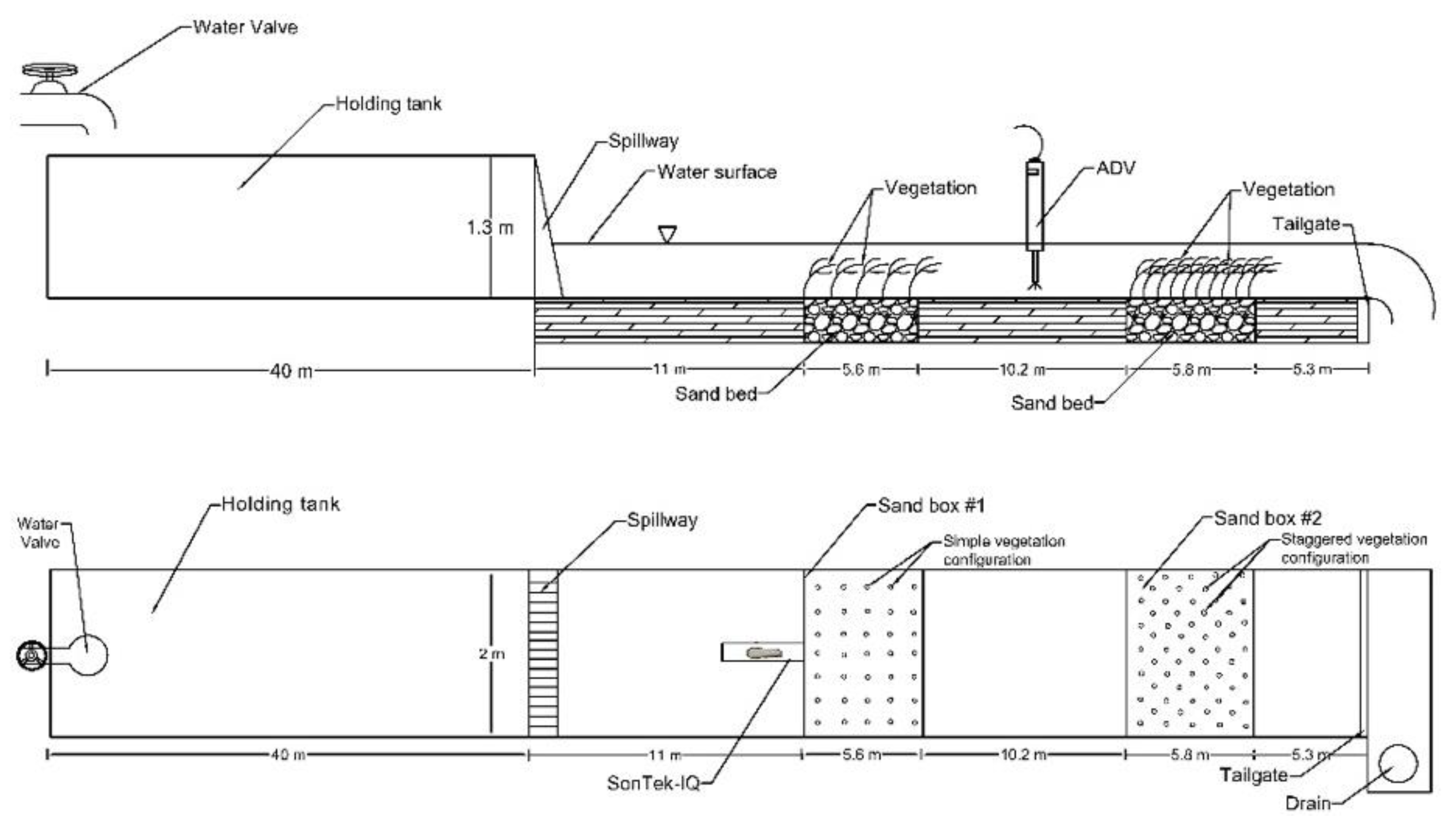
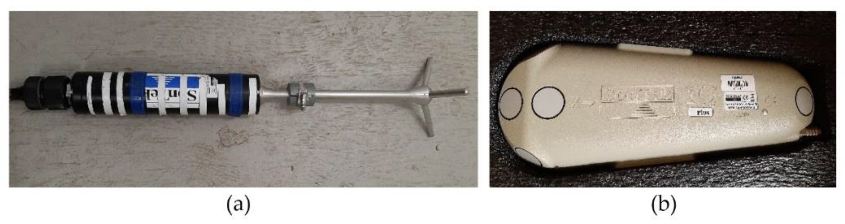
2.1. Flume, ADV, and SonTek IQ Used for This Study

Experiments have been carried out in a large-scale outdoor flume. This flume is 38 m long, 2.0 m wide, and 1.3 m deep, as shown in Figure 1. The longitudinal slope of the flume bed was 0.2%. Two water depths of 20 cm and 30 cm have been used for this experimental study by adjusting the tailgates at the end of the flume. These water depths were chosen based on a real situation in nature since the submerged vegetation typically grows in shallow regions of rivers. Flowing water was supplied by a pump and three valves that feed the upstream holding tank. Water in the holding tank upstream of the main channel was maintained at a constant water level. The desired constant flow rate, which is 100 cm³/s in this study, was obtained by adjusting these three valves. The holding tank has a volume of 90 m³ to keep a constant water level during each experimental run.

The aspect ratio W/H is defined as the ratio of the flume width to water depth. For both water depths of 20 cm and 30 cm used in this experimental study, the flume is classified as a wide flume since the aspect ratio is greater than 5 to 10. This means that in this flume, the effects of the side walls of the channel and the secondary currents can be ignored in the center zone of the flume [30].

There were two sandboxes which are spaced 10.2 m from each other. These sandboxes were 2 m wide and 0.3 m deep. The upstream sandbox was 5.6 m long and the downstream one was 5.8 m long.

In this experimental study, a down-looking Acoustic Doppler Velocimeter (ADV) 10-MHz, developed by Nortek, was used to measure the instantaneous three-dimensional velocity components with a sampling rate of 25 Hz and a sampling volume of 0.25 cc (Figure 2a). The duration of each measurement was 2 min, acquiring 3000 instantaneous velocity data at each measurement point. The vertical intervals between two consecutive points for each velocity profile were 10 mm. The signal-to-noise ratio (SNR) was recorded in the ADV file and used for assessing the strength of the received acoustic signal against the ambient electronic noise level of the ADV [31]. To obtain high-quality data from the ADV, SNR values should be greater than 5 dB for measurements of the mean flow velocity and greater than 15 dB for the instantaneous velocity or turbulence quantities. The filtering method of Goring and Nikora (2002) [32] and Wahl (2002) [33] was selected in this study. The WinADV software was used for data filtering. One of the real-time outputs provided by the ADV is a statistic correlation to assess the quality of the velocity measurements. If the average correlation was less than or equal to 70%, the measured velocity data were filtered out.

Measurements at any depth less than 10 cm from the water surface could not be used due to limitations of the ADV since the distance of the sampling volume in this ADV is located 10 cm below the transmitter. It means that the collected data are from the near bed up to 10 cm below the water surface where the ADV was operational. The fluctuating turbulence near the channel bed is more important than that near water surface. Since most sediment transport caused by drag force resulted from vegetation elements and bed shear stress occurs closer to bed [34,35], one can conclude that the limitation of the ADV for measuring the fluctuations from water surface to 10 cm below it does not affect the results much.

After removing spikes using the WinADV software, velocity fluctuation in the longitudinal (x), lateral (y), and vertical (z) directions were calculated as follows:

$$\begin{array}{c}{u}^{\prime }=u_i-u\\ v^{\prime }=v_i-v\\ w^{\prime }=w_i-w\end{array}$$

(1)

where u, v, and w are the time-averaged velocities that correspond to the directions x, y, and z, respectively; $u_i$, $v_i$, and $w_i$ are the instantaneous velocities that correspond to the directions x, y, and z, respectively. The x axis is aligned with the direction of the mean flow. The y axis is the spanwise direction, and the z axis is vertical, with z = 0 at the channel bed, and positive upward.

The equilibrium state of the scour process in vegetated channels will achieve after 48 h [36]. To make sure that the exact flow rate has been obtained over the duration of 48 h, a SonTek-IQ Plus was used (Figure 2b). This precise and robust apparatus was also used to measure the average velocity and water depth with advanced post-processing functions [37]. The SonTek IQ is a semi-rectangular shape designed to mount on the channel bottom. Because of the sleek silhouette of the SonTek IQ, its impact on flow is minimal. The surface slope $\partial H/\partial x$ was measured using a staff gauge installed in the middle of the sandbox to verify the water depth manually.

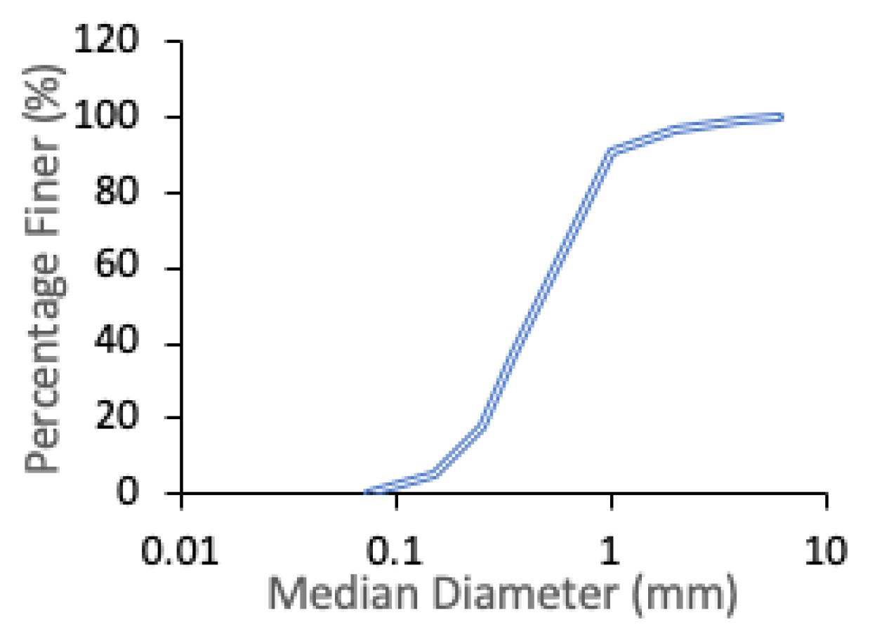
2.2. Sediment Used in Experiments

The sandbox is filled with non-uniform sediment with a median particle size ($D_{50}$) of 0.50 mm. The standard deviation ($\sigma =\sqrt{D_{84}/D_{16}}$) was used to analyze the uniformity of the distributions where $D_{84}$ and $D_{16}$ are 84% and 16% finer particle diameters, respectively. The smaller the value of $\sigma$, the more well-sorted the sediment is [38]. The standard deviation for the sand with median grain size of 0.50 mm in this study is 1.97. Based on that, the sand size used in this experiment is non-uniform. The grain size distribution was obtained using a mechanical shaker and seven different-sized sieves. Figure 3 shows the grain size distributions of the bed material.

The following equation proposed by Hager (1999) is used for determining the roughness coefficient of the channel bed [39]:

$$n_b=0.039D_{50}^{\left(1/6\right)}$$

(2)

where $n_b$ is the roughness coefficient of the channel bed and $D_{50}$ is median grain size of sediment particle. Therefore, the roughness coefficient of sand bed, $n_b$, is estimated as 0.011 for $D_{50}$ = 0.0005 m.

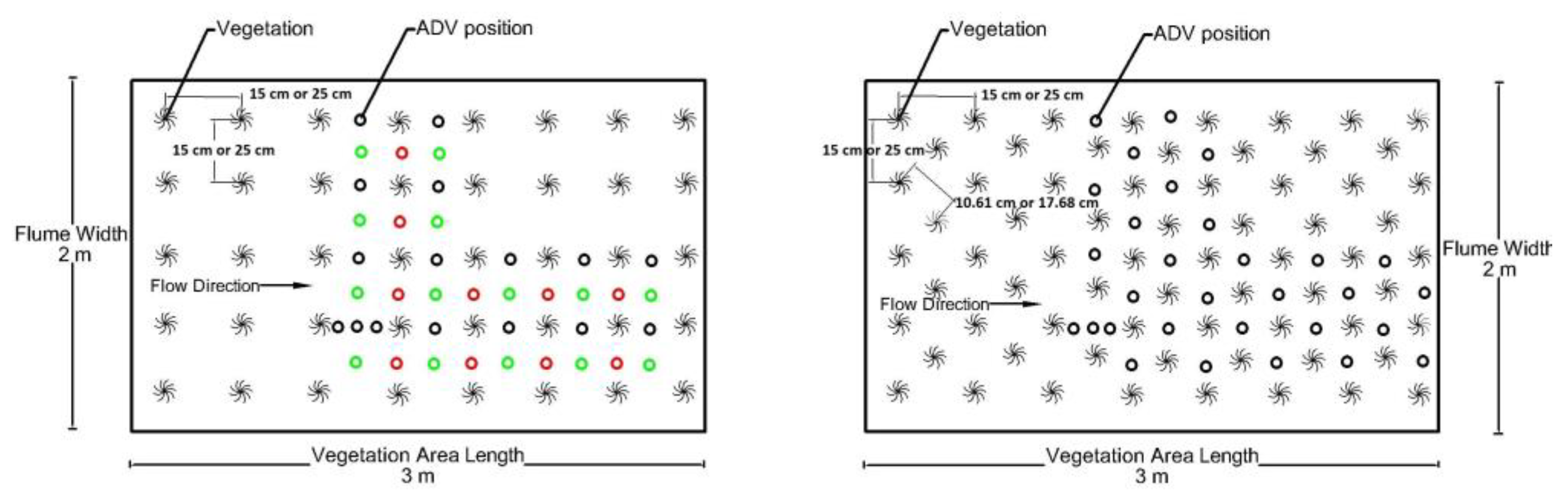
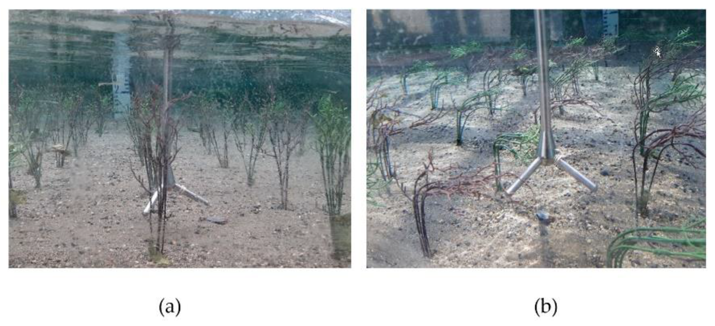
2.3. Vegetation Settings

The model flexible vegetation elements used in this study are made of plastic material. The selected artificial vegetation flexibility is commensurate with the geometry and flexural rigidity of typical aquatic vegetation growing in natural rivers. Each vegetation element consisted of five blades attached to it. Every vegetation element was attached to a grid mesh panel with the spacing distances respectively of 15 cm and 25 cm in a square configuration, and 10.61 cm and 17.68 cm in a staggered configuration. Then, the grid mesh panel with vegetation elements was placed and buried 10 cm below the sand bed surface. Afterward, the surface of the sandbox with vegetation was carefully leveled. By doing so, the vegetation elements were fully stabilized in the sand, representing a natural situation with roots in channel bed.

Figure 4 shows the positions for measurement using an ADV (ADV positions) in channel bed with two different vegetation arrangement patterns, namely, the square and staggered configurations. Measurements at 24 ADV positions around vegetation elements provide robust information for detecting flow structure and turbulence. To determine the wake structure behind each vegetation element, the velocity profile was taken at three points in the wakes of some vegetation elements, as shown in Figure 4.

The flowing water from upstream passes through the submerged vegetation patch. After a certain distance from the upstream edge of the submerged vegetation patch, the flow will be fully developed. Upstream of submerged vegetation, flow follows boundary layer conditions. Once the flow approaches submerged vegetation, this condition turns into a mixing layer. In the mixing layer flow, the shear layer known as Kelvin–Helmholtz vortices will be developed and reaches an equilibrium in size depending on the vegetation density and submergence ratio [40]. The flow within the submerged vegetation is fully developed when equilibrium is achieved. In this study, all velocity profiles are collected using the ADV in the fully developed flow inside of the vegetation patch, which is different from the fully developed flow in channels without the presence of vegetation.

In the presence of a finite vegetation patch, channel resistance and conveyance are modified, at least locally, resulting in a deviation from uniform flow conditions [41]. In addition, the channel has a longitudinal slope of 0.2% and the bed material is non-uniform sand, which leads to non-uniform flow in the experiment.

The canopy zone can be divided into two sub-zones: the longitudinal exchange zone ($z<h_p)$ and vertical exchange zone ($z>h_p)$ (where z is vertical distance from the bed and $h_p$ is penetration depth). The penetration depth ($z=h_p)$ is defined as the point into the canopy where shear stress decays to 10% of its maximum value. As canopy density increases (ahC_D > 0.2), the penetration depth decreases [42]. Note that C_D is the drag coefficient of vegetation, a is vegetation density a ($m^{-1}$), and $h$ is the bending height of vegetation. The canopy becomes less ventilated since eddies no longer enter the bed [43]. The designated momentum in the longitudinal exchange zone is a balance of pressure gradient or bed slope and vegetative drag. Turbulence in this region is generated at stem wakes and represents the stem morphology. However, in the vertical exchange zone, flow is affected by momentum balance, contributes to scalar exchange, and turbulence is generated by the KH instabilities [44]. In other words, the difference in drag magnitude between the non-vegetated and vegetated zones leads to the Kelvin–Helmholtz (KH) vortices occurring at the interface between vegetated zones and water. The KH vortices can promote the mass and momentum transport within and over canopies [44,45]. For instance, turbulent mass exchange across the canopy–water interface can regulate the nutrients and contaminants.

To investigate the influence of vegetation density on flow structure, artificial vegetation with densities of 16, 32, 36, and 72 stems/$m^2$ were used in this study. It may be sufficient to parameterize vegetation based on stem diameter, density, and the number of plants per area for flow without leaf and non-bending vegetation [46,47].

The vegetation density a ($m^{-1}$) was determined by dividing the projected vegetation area by the vegetation volume (Equation (3)) as [48]:

$$a=\frac{A}{V}=\frac{n{\overline{A}}_i}{WhL}$$

(3)

where n is the amount of vegetation in the area of (W * L), W is the channel width, ${\overline{A}}_i$ is the mean frontal vegetal area, h is the vegetation bending height, and L is the length of channel in which n was counted. Considering five blades per vegetation element, the vegetation density a varies from 0.256 m⁻¹ to 1.2 m⁻¹. Finally, a non-dimensional measure of the canopy density $\lambda =ah$, known as the roughness density, was calculated. The frontal area of vegetation was determined using an image analysis software. This software was designed to distinguish between black and white zones to calculate the silhouette of the vegetation. According to Belcher et al. (2003), there is a scale to distinguish sparse and dense vegetation [29]. In a sparse regime (λ = ah < 0.1), the vegetation drag is small compared to the bed roughness. Therefore, flow velocity acts following the boundary layer profile. In this regime, the turbulence near the bed will increase as the stem density increases. On the other hand, in dense vegetation regime (λ = ah > 0.1), the vegetation drag is clearly high compared to the bed stress. An increase in the vegetation density will lead to a decreased near-bed turbulence and increased sedimentation. The vegetation density in this study is summarized in

Table 1. Vegetation density parameters in this study.

Configuration of Vegetation Elements	Vegetation Density $\mathit{a}\left({\mathit{m}}^{-1}\right)$	Canopy Density (λ = ah)
Square non-bending	0.624	0.12
Square deflected		0.09
Staggered non-bending	1.2	0.23
Staggered deflected		0.17
Square non-bending	0.256	0.05
Square deflected		0.04
Staggered non-bending	0.506	0.1
Staggered deflected		0.07

. One can see from Table 1 that the range of the canopy density λ = ah is 0.04 < λ ≈< 0.23. Some researchers found that, for 0.1 < λ ≈< 0.2, the eddies in the mixing layer penetrate toward the bed. In this study, the vortices (eddies) in the middle layer of the flow, named the mixing layer, penetrate toward the bed and are responsible for turbulence patterns across the vegetation, benefiting the resuspension of sediment [49,50]. As a result, no penetration depth needs to be calculated in the present study because the eddies reach the bed.

Some researchers used the inflexible and idealized cylinders to represent vegetation to investigate the complicated flow structure caused by vegetation; it is unable to fully predict the behavior of natural vegetation due to its differences in roughness, flexibility, and drag coefficient. Besides, flow structure around a single cylinder or vegetation element cannot be generalized for a vegetation patch since a group of cylinders or vegetation elements interact with each other and on flow structure through sheltering effect, blocking effects, and flow separation. Compared to a single cylinder, turbulent fluctuations in the wakes of upstream elements introduce additional kinetic energy to the boundary layer of each element, delaying separation and reducing drag coefficient [47,51]. Therefore, properly characterizing morphological properties of vegetation is essential for studying the hydrodynamics of vegetated streams. To investigate the effect of the flexibility and height of vegetation on flow, both deflected and non-bending morphology of vegetation were used in this study (Figure 5). In one of these vegetation settings, all vegetation elements were placed in a fully non-bending setting to represent the stiff and rigid vegetation patch (Figure 5a). In this way, the vegetation exhibits no deformation during the experiments, representing the real situation of reeds and sedges in natural rivers. In another setting, all vegetation elements were deflected, representing the flexible vegetation in streams (Figure 5b). The height of non-bending and deflected vegetation elements in 20 cm water depth was 12.6 cm and 8 cm, respectively, and 19 cm and 12 cm in the 30 cm water depth. As you saw in Figure 1, the length of each sandbox is around 5.5 m. The 3 m long vegetation region was located in the middle of the sandbox. The vegetation has a certain degree of flexibility and can swing under flow, but it does not deform. The morphological properties of the vegetation such as the vegetation deflected height are related to some other hydraulic properties of flow such as flow depth and velocity.

The ratio of the flow depth to the vegetation bending height is defined as the degree of submergence ($Sr=H/h$) [52]. Thus, the degree of submerged vegetation in this study were selected as 1.58 for non-bending and 2.5 for deflected vegetation arrangement, respectively.

Each vegetation element has the width of 10 mm at the bottom and 22 mm at the top, respectively. Thus, average width of each element was considered as 16 mm. In the present study, for the case of the densest vegetation configuration, the ratio of the total vegetation thickness to the channel width, D/W, was smaller than 0.5; therefore, the effect of channel blockage on the wake structure can be negligible.

The vegetation Reynolds number associated is defined as:

$$R{e}_d=\frac{Ud}{\upsilon }$$

(4)

where $U$ is the mean flow velocity, d is the stem diameter, and $\upsilon$ is the kinematic viscosity of water.

$$F_r=\frac{U}{\sqrt{gH}}$$

(5)

where g is the gravitational acceleration and H is the water depth. Both calculated Reynolds numbers and Froude numbers indicated that the flow was fully turbulent and subcritical for all cases; therefore, no dependence on Fr number was expected.

To start each experimental run, one valve with the low discharge (5 L/s) was gradually opened while the tailgates downstream were closed to avoid sediment being washed away. From the holding tank, water was gently discharged through the spillway into the flume. To maintain the desired flow rate, all three valves were fully opened once the desired water depth was reached. In this study, 32 experimental runs have been conducted including two different submergence ratios, four different vegetation densities with two different layouts including square and staggered configurations for two flow depths of 20 cm and 30 cm. Some of the measured hydraulic data for the flow depth of 20 cm are presented in

Table 2. Some data for the flow depth of 20 cm.

Configuration	$\mathbf{Density}\mathbf{ }\mathbf{(}\mathbf{Stem}\mathbf{/}{\mathit{m}}^{\mathbf{2}}\mathbf{)}$	Flexibility	U (cm/s)	$\mathit{R}{\mathit{e}}_{\mathit{d}}$	λ	${\mathit{u}}_{*}$ (cm/s)	h/H
square	16	deflected	15.15	2423.52	0.0487	3.08	2
		non-bending	17.31	2770.35	0.0359	2.94	1.3
	36	deflected	14.87	2378.56	0.0874	3.42	2
		non-bending	17.58	2813.30	0.1186	3.49	1.3
staggered	32	deflected	14.73	2356.67	0.0961	2.56	2
		non-bending	18.11	2897.52	0.0709	3.16	1.3
	72	deflected	12.46	1993.90	0.168	2.68	2
		non-bending	16.93	2708.75	0.228	3.49	1.3

.

3. Results and Discussions

3.1. Velocity

In this study, the values of shear velocity ($u_{*}$) were obtained using the boundary layer method [53]:

$$u_{*}=\frac{\left({\delta }_{*}-\theta \right) u_{max}}{C{\delta }_{*} }$$

(6)

where u_max is maximum streamlined velocity, and C is an empirical constant that was found to be equal to 4.4 in laboratory experiments [53]. The parameter ${\delta }_{*}$ is the boundary layer displacement thickness and indicates the distance by which the external streamlines are shifted owing to the formation of the boundary layer. It is impossible to present a boundary layer thickness in an unambiguous way because the effect of viscosity in the boundary layer decreases asymptotically outwards [54]. In order to avoid utilization of an arbitrary boundary layer thickness, it is necessary to consider the boundary layer displacement thickness, ${\delta }_{*}$ [55]:

$${\delta }_{*}={{\displaystyle \int }}_0^H\left(1-\frac{u}{u_{max}}\right)dz$$

(7)

where u is the mean point velocity at a distance z measured from the reference level. Furthermore, the momentum thickness (θ) in Equation (6) indicates the loss of momentum in the boundary layer as compared with potential flow and is defined as:

$$\theta ={{\displaystyle \int }}_0^H\frac{u}{u_{max}}\left(1-\frac{u}{u_{max}}\right)dz$$

(8)

The exact values of ${\delta }_{*}$ and θ depend upon the distribution of downstream velocity at the cross-section normal to the flow.

In a channel with the presence of vegetation, there is an inner layer called the emergent zone that is controlled by stem scale turbulence. Above that layer, there is a layer with Kelvin–Helmholtz (KH) vorticities that dominate mass and momentum exchange. The logarithmic layer refers to the upper layer of turbulent flow where the velocity profile follows a log shape [56]. Kazem et al., 2021, reported these three layers were present in all cases of their experiments [57]. The logarithmic profile may be described by the Karman–Prandtl equation:

$$u=u_{*}\left(Ln\frac{z-{\delta }_{*} }{z_0}\right)/\kappa$$

(9)

where $u_{*}$ is the shear velocity, z₀ is the roughness height, and κ is the von Karman constant, which is 0.41. The value of ${\delta }_{*}$ was determined to be 0.02 m through Equation (7) for non-bending vegetation and 0.03 for deflected vegetation. In this study, z₀ is assumed to be equal to D₅₀.

Results of the velocity showed there are significant differences by changing the density, morphology, and layout of vegetation. In addition, velocity is affected by both the measurement position and water depth using an ADV.

Figure 6 shows velocity profiles in the presence of a deflected and non-bended vegetation patch in the channel bed. One can see from this figure that these velocity profiles deviate from the logarithmic law distribution (the Karman–Prandtl Equation) and are confined to the upper part of the flow in the presence of the vegetation patch. In addition, there exists a very good correlation-ship between u/$u_{*}$ and (z − ${\delta }_{*}$)/z₀. Note: a logarithmic profile in the flow’s inner layer cannot be developed due to the presence of vegetation [58].

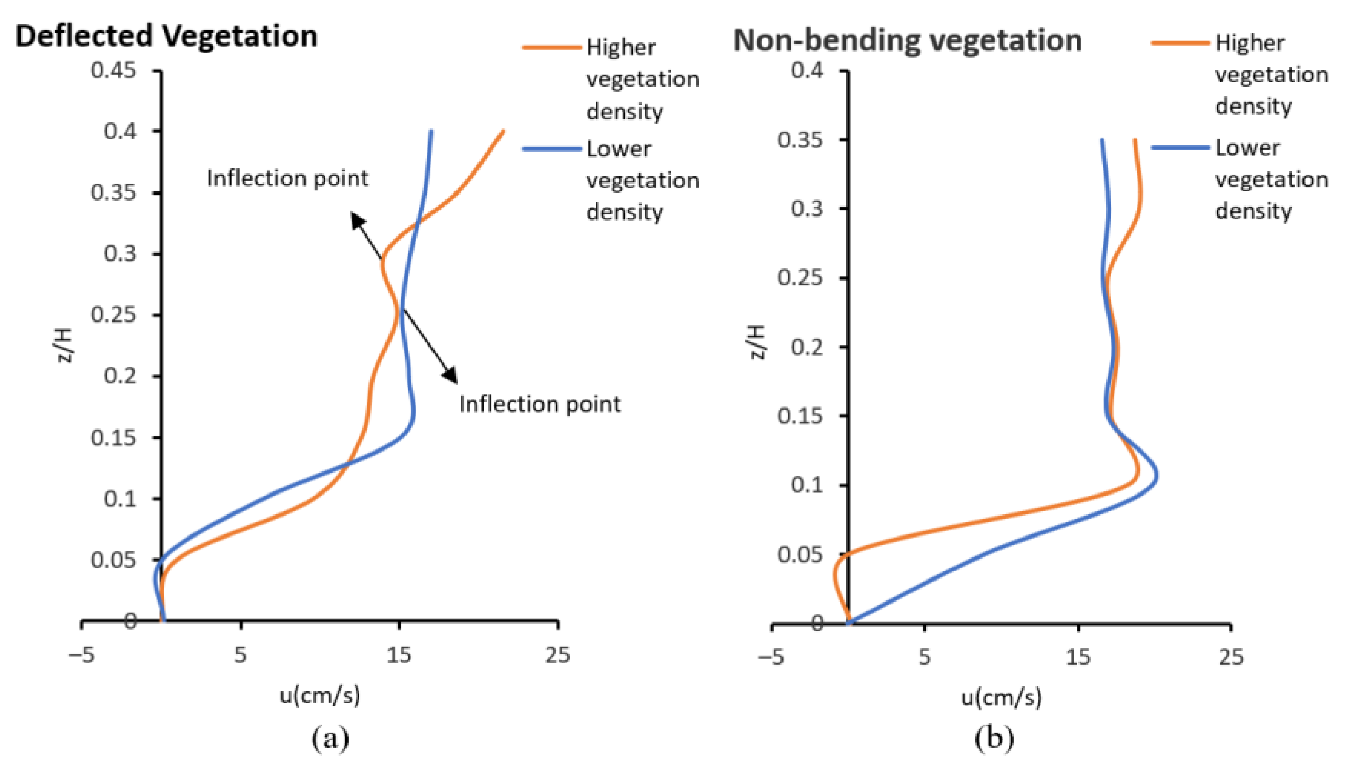
3.1.1. Effects of Vegetation Density on Streamwise Velocity

The velocity profiles for the different vegetation densities in the fully developed region are compared, as shown in Figure 7. One can observe from Figure 7 that with the increase in the vegetation density (a = 0.624 $m^{-1}$), the flow velocity within the canopy decreases, and correspondingly the flow velocity above the canopy increases.

In the rear of the vegetation wake zone, vegetation creates resistance to flow, and causes flow separation and a decrease in flow velocity near the bed. This phenomenon is the main reason for sediment retention especially behind the deflected vegetation patch with high density. Although this statement is generally true, scour holes around vegetation stems have been observed in many studies and are dependent on vegetation density. Vegetation deflection can be viewed as a passive “drag-reduction” strategy exhibited by vegetation. As shown in Figure 7, the inflection points at the top of the deflected vegetation in the wake zone behind the vegetation are sensible (see arrows in Figure 7a). This finding is in good agreement with that of other researchers that velocity profiles in flows with submerged vegetation contain an inflection point near the top of the vegetation [42,59]. There is an increase in velocity on top of the canopy of the deflected vegetation at z/H = 0.4 compared to the inner layer of vegetation. The difference between the drag magnitude in the non-vegetated zone and that in the vegetated zone causes the Kelvin–Helmholtz (KH) vortices at the interface between vegetation and non-vegetation layer. The KH vortices promote mass and momentum transport both within and over canopies [44,45,47]. The KH instabilities significantly affect the large-scale turbulence structures and the momentum transfer between the non-vegetated and vegetated regimes. The effects of KH instabilities show their effect as an inflection point in velocity profiles [42,59]. Decreasing deflected vegetation spacing (i.e., increasing canopy density) largely retards streamwise velocity at (z/H ≅ 0.3), slightly below the inflection point (see Figure 7a). The inflectional region tends to disappear when the canopy becomes sparser resulting in an increase of the shear length scale associated with the velocity field. Non-bending vegetation lacks this.

On the other hand, in the presence of the non-bending vegetation in the channel bed, for the sparsest vegetation (a = 0.256 $m^{-1}$), the highest velocity occurs near the bed and lowest velocity near water surface. The peak velocity occurs at the depth of z/H = 0.1, that is, the sheath section where the frontal width is minimal. Because the sheath section is more porous than the middle vegetated layer, it can handle larger flows [11]. A high negative velocity gradient happened from z/H = 0.1 to z/H = 0.15. Then, a decreasing trend of velocity to the water surface is noticeable.

According to Figure 7, it is suggested that the dense deflected vegetation (λ ≥ 0.1) results in the decrease in sediment transport in streams by reducing the velocity near the bed more than non-bending vegetation and sparse densities. Therefore, it is suggested that dense vegetation provides better protection for beds subject to erosion and scour.

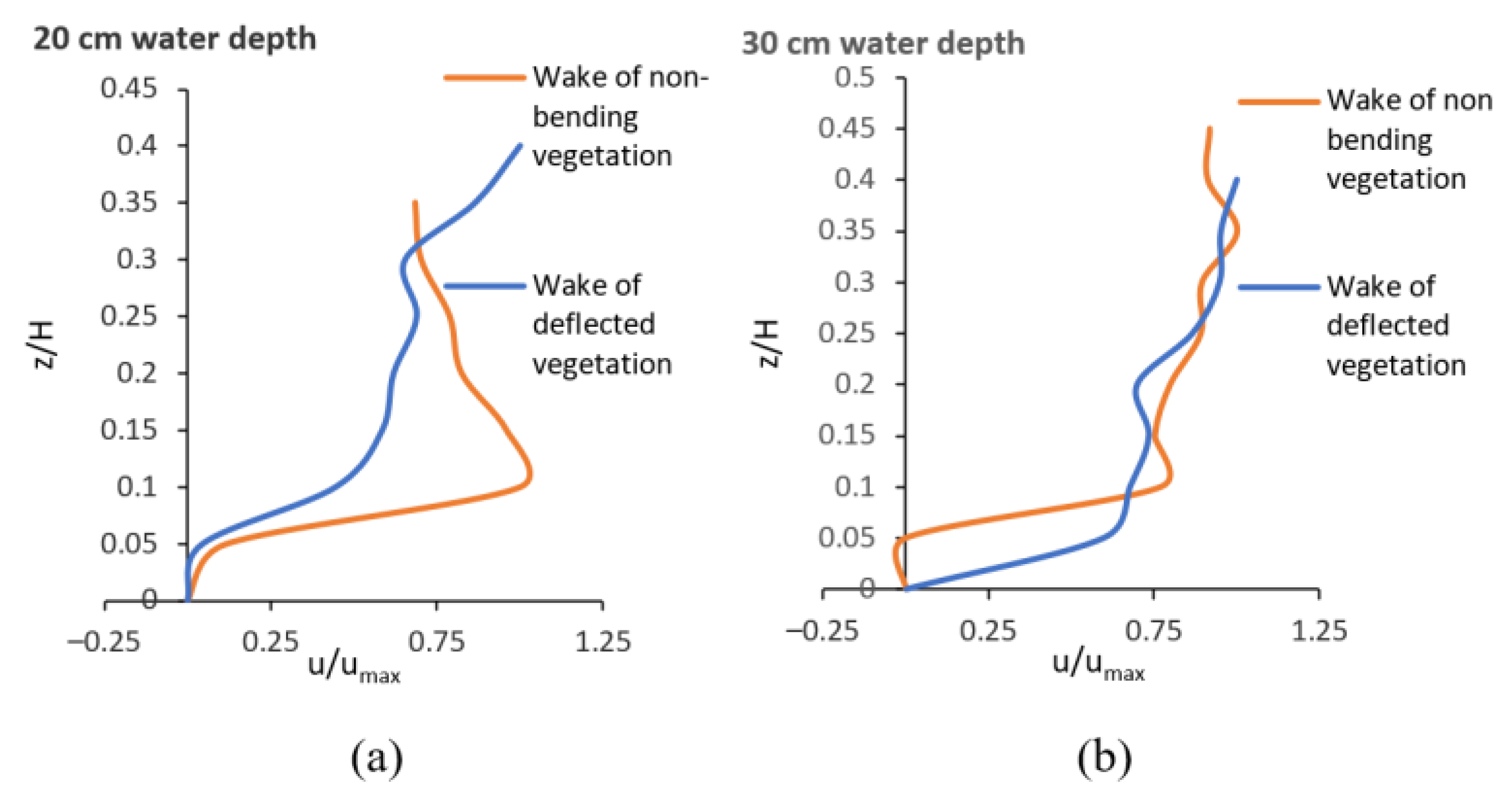
3.1.2. Effects of Water Depth of Streamwise Velocity

In the presence of non-bending vegetation in the channel bed with the flow depth of 20 cm, a high velocity gradient has been observed from the channel bed z/H = 0 to the depth of z/H = 0.1 where a peak velocity was reached. After this depth, a decreasing trend of velocity toward the water surface (when 0.1 < z/H < 1.0) is noticeable (Figure 8). However, for the deeper flow of 30 cm, the peak velocity occurs at a larger distance from the channel bed but closer to the water surface. It has also been noticed that, from the depth of z/H = 0.1 to the water surface, the value of flow velocity does not change. The dip phenomenon (the position at which the maximum velocity appears below the water surface) was observed for the case of the non-bending vegetation.

In the wake zone of deflected vegetation, the velocity in the inner layer of 20 cm-depth flow is less than that in the 30 cm-depth flow, and the velocity in the upper layer in the 20 cm-depth flow is more than that in the 30 cm-depth flow. It can be concluded that, by keeping the same submergence ratio, the shallower the flow depth, the lower the flow velocity in the inner layer in the wake zone of deflected vegetation, and the higher the flow velocity in the outer layer.

Thus, both the flow depth and morphology of vegetation have a substantial effect on the velocity profile. For the non-bending vegetation case, a peak velocity value appears near the bed in shallow water, implying that the non-bending vegetation acts like an emergent vegetation. Therefore, fine sediment particles cannot be easily retained behind the vegetation patch due to high flow velocities. In contrast, in the presence of deflected vegetation in a channel bed, the velocity near bed is smaller than that of non-bending vegetation mainly due to the sheltering effect behind vegetation (see Section 3.2. Turbulence Kinetic Energy for more information). In a deeper flow (30 cm), the peak velocity is shifted toward the water surface compared to that in a shallower flow (20 cm) with high velocity near the channel bed. As a consequence, sediment deposition is more probable in a deeper flow comparing to that in a shallower flow.

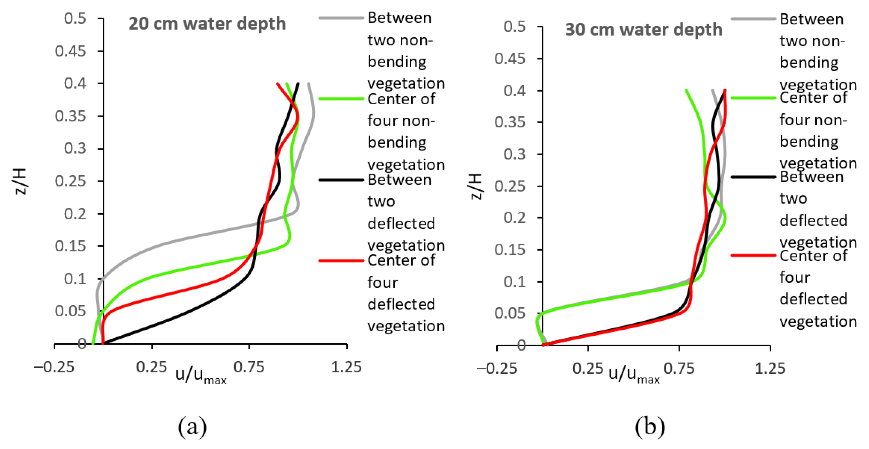
3.1.3. Effects of Square Arrangement on Velocity Profile

Figure 9 shows the dimensionless time-averaged streamwise velocity distribution between two vegetation elements (red circles in Figure 4) and in the center of four vegetation elements (green circles in Figure 4) with a density of a = 0.624 $m^{-1}$ in the flow with the depth of 20 cm compared to that in the flow with the depth of 30 cm.

In the presence of dense non-bending vegetation with a square arrangement pattern in the channel bed, for the flow with a depth of 20 cm, the difference between mean streamwise velocities in the middle of two vegetation elements and those in the wake of vegetation elements is 27.39%; and the difference between mean streamwise velocities in the center of four vegetation elements and those in the wake of vegetation elements is 30.64%. In the presence of dense deflected vegetation in the channel bed, these values are 26.79% and 28.08%, respectively. For the flow with a depth of 30 cm, the same trend was calculated. According to these results, in the presence of dense vegetation of λ ≥ 0.1, the velocity in the middle of two vegetation elements is lower than that in the center of four vegetation elements. Accordingly, in vegetation with a high density, the width of the wake behind the vegetation is narrow, leading to the increase in the flow velocity in the center of the vegetation elements. In other words, the vegetation with a high density reduces the flow cross-sectional area locally, and thus results in a narrow wake behind the vegetation which diminishes faster within a shorter distance compared to that for the case of sparse vegetation. In contrast, in the presence of sparse non-bending vegetation with low density (i.e., λ < 0.1) in the flow with a depth of 20 cm, the difference between the mean streamwise velocities in the middle of two vegetation elements and those in the wake of vegetation elements is 20.56%; and the difference between the mean streamwise velocities in the center of four vegetation elements and those in the wake of vegetation elements is 12.05%. For the case of deflected vegetation, these differences are 34.48% and 33.75%, respectively. The same trend was observed in the flow with a depth of 30 cm. This finding shows that, in the presence of sparse vegetation in the bed, the mean streamwise velocity in the middle of two vegetation elements is higher than that in the center of four vegetation elements. This effect indicates the presence of a wide wake behind each vegetation element that attenuates the velocity at the center of four vegetation elements.

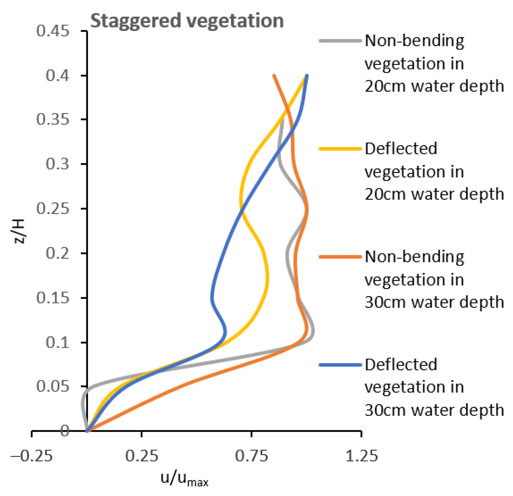
3.1.4. Effects of Staggered Arrangement on Velocity Profile

Figure 10 shows the velocity profiles in the presence of both deflected and non-bending vegetation arranged in a staggered layout in flows with different depths of 20 cm and 30 cm, respectively. The characteristics of velocity profiles of flow in the presence of vegetation with a staggered arrangement follow the same trend as those of velocity profiles in the wake of vegetation arranged in a square configuration, as discussed above. However, velocity profiles are more inflectional in vegetation with a staggered arrangement compared to square arrangement. As one can see from Figure 10, the velocity profile for the case of the staggered vegetation arrangement in the wake of deflected vegetation has an “S” shape. In the middle part close to the leaf zone of vegetation, the flow velocity reaches its maximum. In this zone, the drag force causes an appreciable retardation of the mean velocity; in the flow with a depth of 30 cm, this zone is located at 0.1 < z/H < 0.15, and in the flow with a depth of 20 cm, this zone is located at 0.15 < z/H < 0.25. As the velocity increases with the distance above the vegetation zone, the drag resulted from vegetation gradually diminishes, and the shear stresses decline until zero at the free water surface.

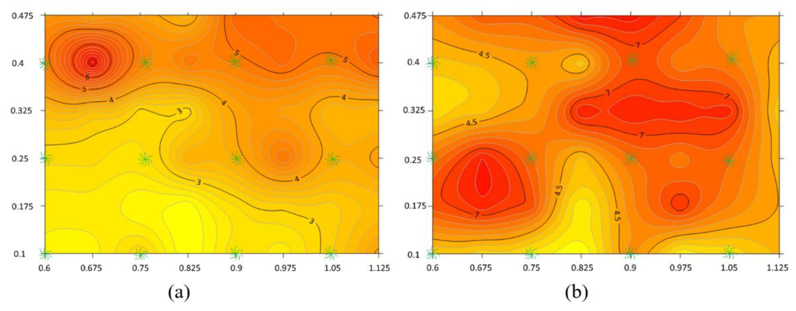
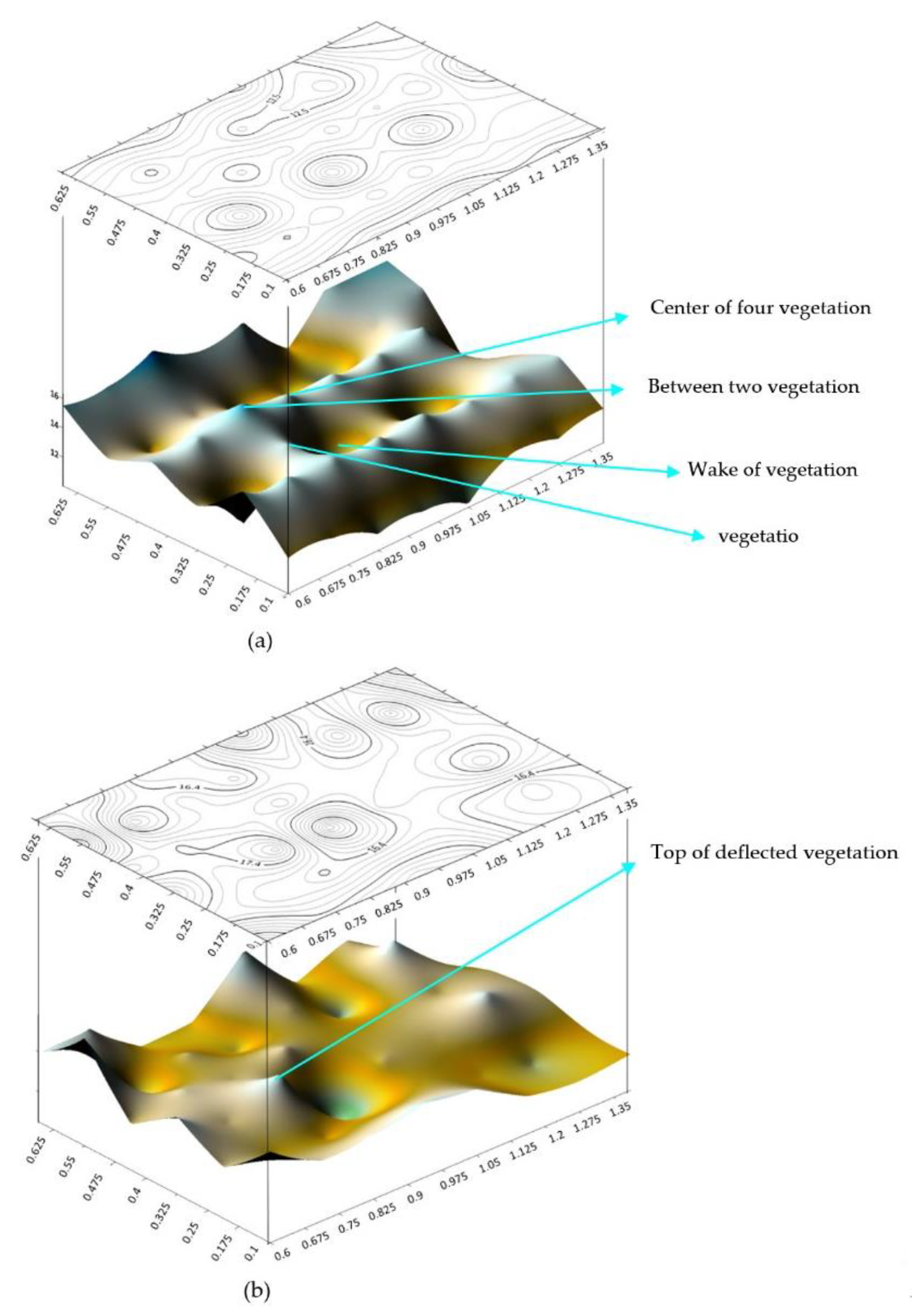
3.1.5. Velocity Contours in Square Arrangement

In Figure 11, two-dimensional and three-dimensional velocity contours are presented near the bed (at a depth of z/H = 0.1) and at the top of deflected vegetation (at a depth of z/H = 0.4). The depression spot in the contours in Figure 11a illustrates the wake zone of vegetation in the separation flow zone where sediment deposition was observed. Near the bed, velocity is higher between rows of vegetation elements. These graphs demonstrate that velocity in the center of the square formed by four vegetation elements is lower than that in the middle two vegetation elements. This figure confirms the results of Section 3.1.3. Some spikes in Figure 11b indicate high velocities at the interface between the deflected vegetation and non-vegetation layer as inflection points in velocity profiles compared to its neighboring zone.

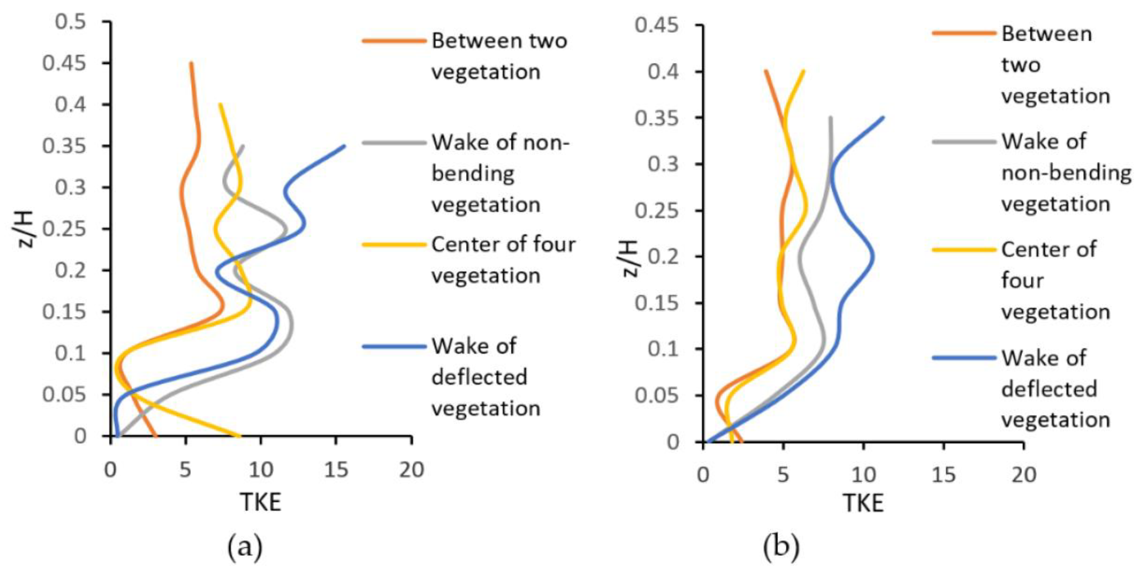
3.2. Turbulence Kinetic Energy (TKE)

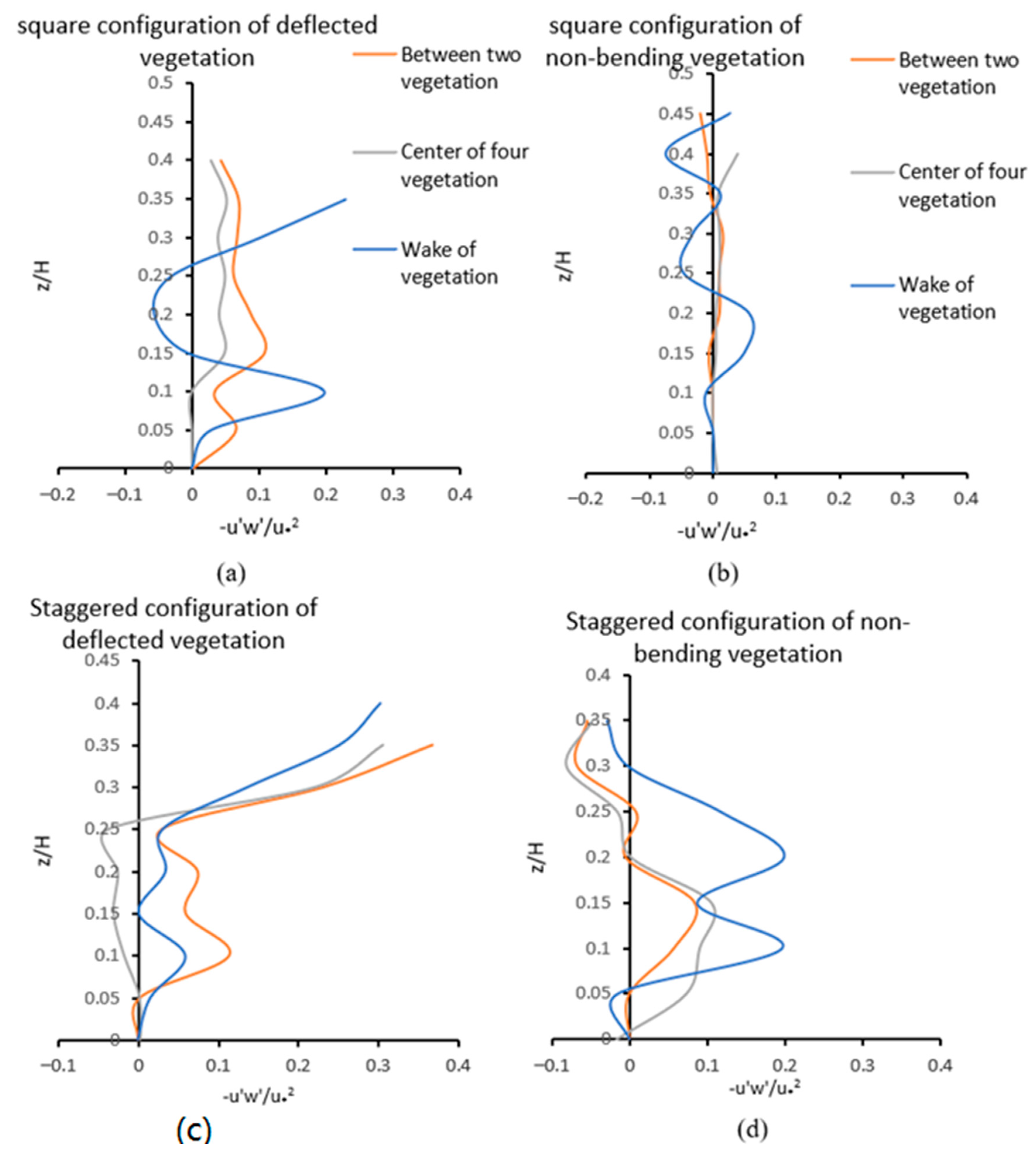
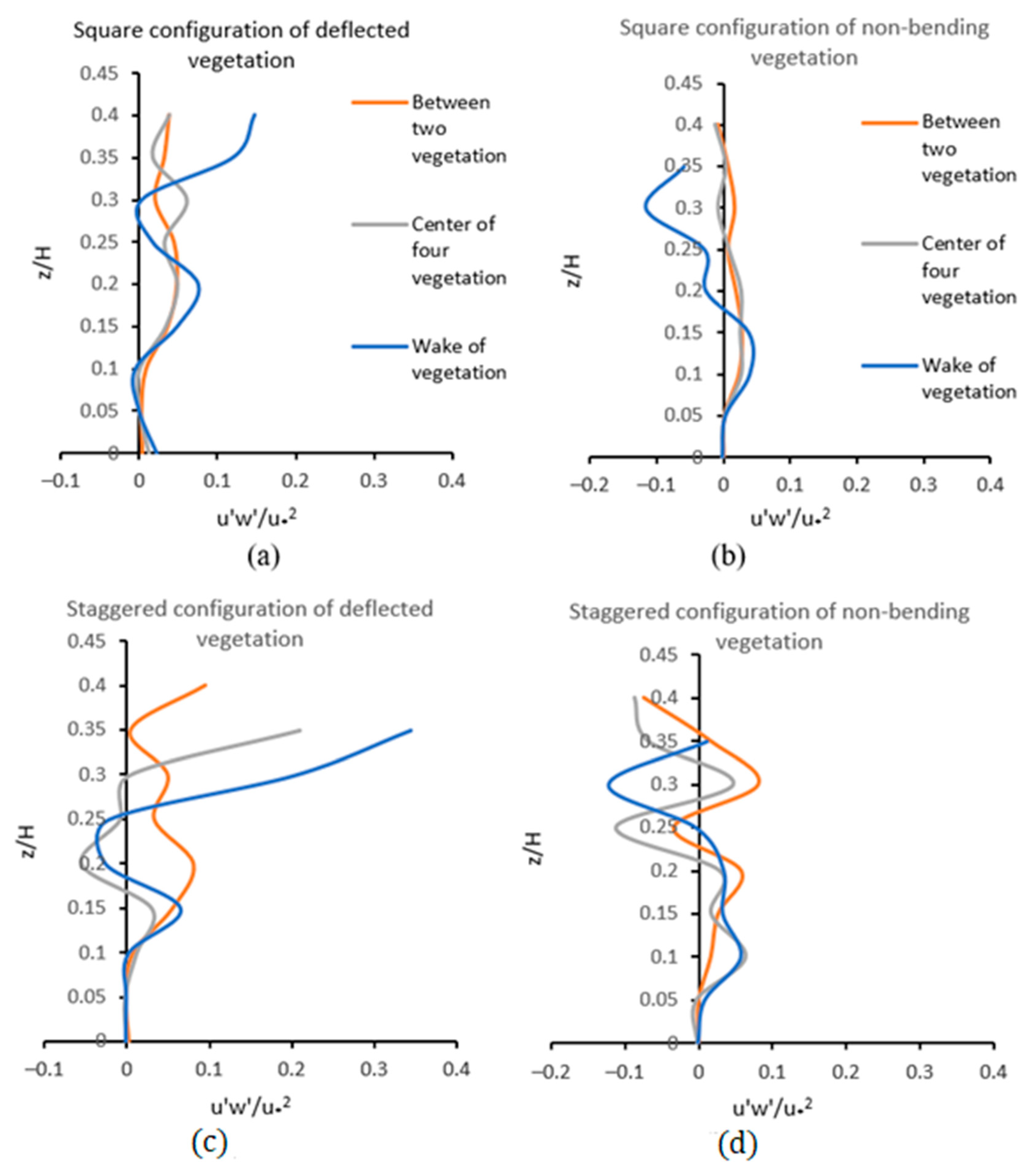
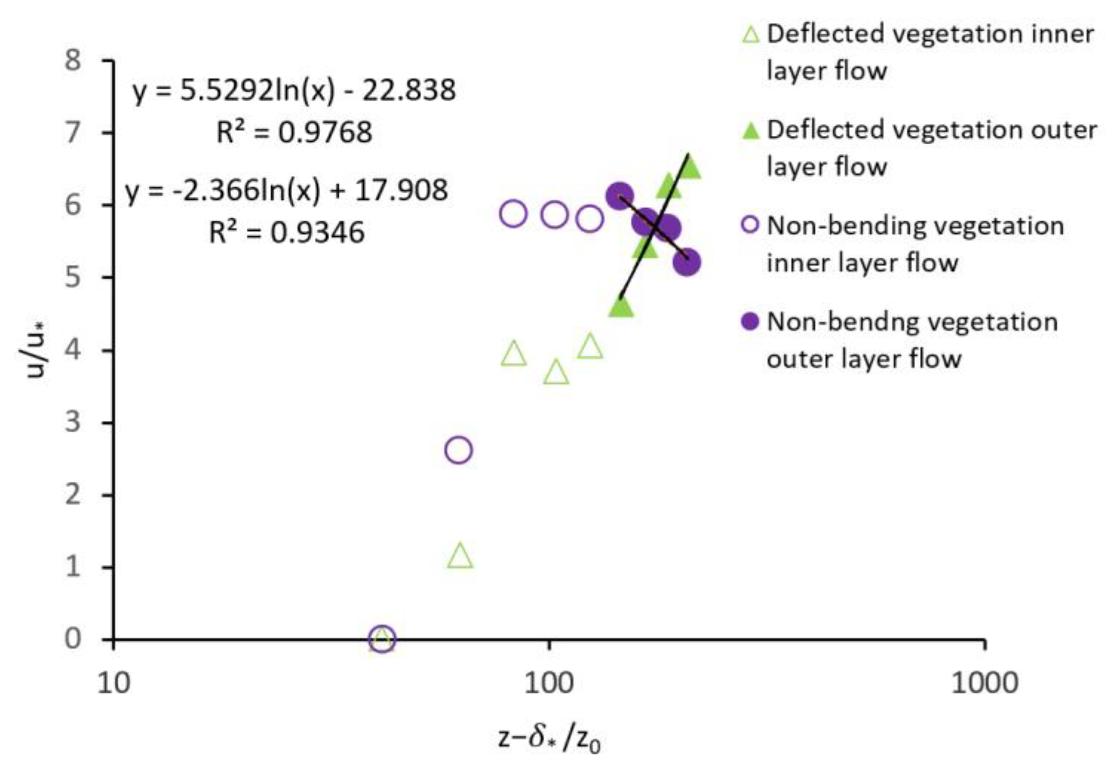
The generation of vortices in the stem wake zone behind vegetation drains energy from the mean flow and feeds it into turbulent kinetic energy (TKE). In this case, turbulent energy is produced at the same rate as the work done by the flow against vegetation drag [60]. Most sediment transport models are based on bed shear stress in a bare channel since turbulence is related to bed stress. However, in vegetated channels, the turbulence level is related to the vegetative drag and has little or no link to the bed shear stress [47].

The local turbulent kinetic energy was defined as

$$\mathrm{TKE}=1/2\left(\overline{{u^{\prime }}^2}+\overline{{v^{\prime }}^2}+\overline{{w^{\prime }}^2}\right)$$

(10)

where $\overline{u\prime }$, $\overline{v\prime }$, and $\overline{w\prime }$ represent the root-mean-square velocity fluctuations (RMS), indicating the mean energy per unit mass related to turbulent eddies in streamwise, lateral, and vertical directions, respectively.

$$\{\begin{array}{c}\mathrm{RMS}\left(u^{\prime }\right)=\overline{u^{\prime }}=\sqrt{\overline{{u^{\prime }}^2}}\\ \mathrm{RMS}\left(v^{\prime }\right)=\overline{v\prime }=\sqrt{\overline{v{\prime }^2}}\\ \mathrm{RMS}\left(w^{\prime }\right)=\overline{w\prime }=\sqrt{\overline{w{\prime }^2}}\end{array}$$

(11)

Compared to that TKE measured between two vegetation elements and those in the center of squares formed by four vegetation elements (vegetation-free streamline), as shown in Figure 12, the TKE was significantly enhanced by vegetation. In this study, this trend will be discussed in greater detail.

The TKE in Figure 12 in the wake of the vegetation depicts that the maximum $\mathrm{RMS}\left(u^{\prime }\right), \mathrm{RMS}\left(v^{\prime }\right), \mathrm{and} \mathrm{RMS}\left(w^{\prime }\right)$ occur either at the sheath section of the vegetation (at the depth of z/H = 0.1) or above the top of the vegetation (at the depth of z/H ≥ 0.4).

In the sheath section, the frontal projected area is small, and flow can mostly pass through the sheath section. Furthermore, stem scale turbulence was boosted at the sheath section. Turbulence generated by individual stem wakes was attributed to the enhancement of TKE behind vegetation at the depth of about z/H = 0.1. The near-bed turbulence kinetic energy is enhanced by both bed-generated and vegetation-generated turbulence in the presence of submerged vegetation. In the region slightly far from the channel bed to the vegetation top, the presence of the von Karman vortex street results in the enhancement of TKE comparing to that in unvegetated channels. Due to the increased turbulent kinetic energy (TKE) associated with the von Karman vortex street, which inhibits sediment deposition, the location of the vortex formation indicates an important transition between zones where net deposition increases and zones where net deposition diminishes compared to those without the presence of vegetation in the bed [61].

On the other hand, there are no obstructions to the flow at the top of the vegetation. Thus, the TKE terms reach their maximum values. This result confirms that of Afzalimehr et al. (2011) [62]. During the transition from the vegetated zone to the unvegetated zone, the kinetic energy has the opportunity to enhance itself.

While in the profiles at the points either between two vegetation elements or in the center of the square formed by four vegetation elements, the TKE near the bed was greater than the TKE behind vegetation elements. As shown in Figure 12, TKE near the bed (z/H = 0) in the wake of vegetation elements starts at zero; however, a TKE between two vegetation elements and in the center of square formed by four vegetation elements (vegetation-free streamlines) does not equal zero (TKE > 0). This is a well-known effect of the submerged vegetation on turbulence, and it is called the sheltering or dampening effect. A sheltering effect occurs when two bodies are positioned so that one is located in the wake of the upstream body [63]. The downstream body experiences a lower approaching velocity than that for the upstream body, resulting in a lower drag force. Depending on how vegetation elements are arranged, the sheltering effect can be relevant to vegetation-covered flows [51].

As shown in Figure 12, the TKE profiles for vegetation densities of a = 0.624 m⁻¹ and a = 0.256 m⁻¹ indicate a greater effect of this phenomenon in denser vegetation due to a shorter distance between vegetation elements (or smaller spacing distance between vegetation elements). Therefore, the sheltering effect is more evident in denser vegetation comparing to that in sparse vegetation. This effect can enhance sediment deposition and protect the bed from erosion [64,65]. Nosrati et al., 2022 [66], found that the bending deformation of vegetation results in a significant reduction in the spacing distance between vegetation elements, causing an intensified sheltering effect and a lower form drag force. The TKE decreases significantly near the bed (0 < z/H < 0.05) in the wake zone of denser vegetation. In addition, with the decrease in the flow depth from 30 cm to 20 cm, the TKE near the bed decreases. Shahmohammadi et al. (2018) [8] found that the TKE in bare channels is greater compared to the upstream-approaching flow from a vegetated channel. Results of the present study are in good agreement with that of Shahmohammadi et al. (2018) [8]: namely, as the vegetation density decreases, the TKE near the bed (z/H = 0) increases.

One can see from Figure 13, in the wake zone behind each vegetation element, the TKE value at the top of the deflected vegetation has a high value, confirming the presence of KH vortices at that flow depth. This result is in agreement with that of Kazem et al. (2021) [67]. In addition, near the channel bed, the high value of TKE took place in the pathway between vegetation elements. This high value of TKE should be the main cause of sediment transport in vegetated channels. It has been noticed from Figure 13b that the TKE has a low value in front of each vegetation element near the bed that was discussed above as a sheltering effect.

3.3. Shear Stress

In this study, the primary turbulent Reynolds Shear Stress (RSS) $\tau$ at a distance from the bed of z was determined from

$$\tau \left(z\right)=-\rho <u^{\prime }{w}^{\prime }>$$

(12)

where $\rho$ is the mass density of fluid, angle brackets denote the spatial average of flow variables, and $u^{\prime }$ and $w^{\prime }$ are instantaneous velocity fluctuations in the longitudinal and vertical directions, respectively. The values of RSS were normalized by the square of shear velocity ($u_{*}^2$).

Results show that the presence of vegetation in a channel bed causes a deviation of the RSS distribution from the linear one. It is also noticed that the RSS distribution is influenced by the aspect ratio (W/H) [62].

In Figure 14, in the presence of vegetation elements with a square arrangement ($a=0.624 m^{-1})$, the RSS has been displayed at the following locations: in the middle of two vegetation elements (red circles in Figure 4), at the center of the square formed by four vegetation elements (green circles in Figure 4), in the wake zone of vegetation elements (black circles in Figure 4), and in the wake zone of vegetation elements with staggered configuration ($a=1.2 m^{-1})$. At the same location as shown in Figure 14, the RSS presents in Figure 15 for vegetation densities of ($a=0.256 m^{-1})$ for a square configuration and ($a=0.506 m^{-1})$ for a staggered configuration of vegetation elements.

Results showed that the RSS is highly affected by vegetation density, morphology, and the place for data collection as displayed in Figure 14 and Figure 15. For the case of non-bending vegetation with a square configuration and density of ($a=0.624 m^{-1}$), the RSS does not change much throughout the flow depth between two vegetation elements, and at the center of the square formed by four vegetation elements with a slight fluctuation pattern (Figure 14 and Figure 15b). Inside the inner layer of the vegetation, however, more fluctuation in shear stress has been noticed with the negative values of RSS near the water surface. The negative values of RSS near the water surface for the non-bending vegetation case are attributed to turbulent fluxes associated with vegetation morphology and negative streamwise velocity gradients (see Figure 9a).

For the deflected vegetation case (Figure 14a), similar to the non-bending vegetation case (Figure 14b), constant RSS through the water depth was observed between two vegetation elements and at the center of the square formed by four vegetation elements. However, the RSS values for the deflected vegetation case are higher than those for the non-bending vegetation case. For the case of deflected vegetation with a square configuration, at the center of the square formed by four vegetation elements and between two vegetation elements (see Figure 14a), the RSS has a maximum value at a depth of z/H = 0.15. However, in the wake zone behind the deflected vegetation, the maximum value of RSS occurred at an elevation slightly higher above the top of the vegetation, indicating the presence of the KH instability at the top of the deflected vegetation and slightly above the top of the vegetation (z/H ≥ 0.4). As one can see from Figure 14a, above the top of the vegetation, the increasing trend of RSS is continuous. The shift of the maximum RSS above the top of the vegetation is caused by the presence of branches that alter the peak of RSS to a higher location above the top of the vegetation. Near the channel bed, the RSS is close to zero and starts to increase around z/H = 0.1, which is associated with stem scale turbulence at this zone. Then, the RSS reaches the peak value at the depth above the vegetation bending height, namely around z/H = 0.4. When the vegetation is deflected, the drag discontinuity at the edge of the vegetation produces a shear layer at this interface. The Kelvin–Helmholtz instability forms large coherent vortices within the shear layer, and these structures dominate vertical transport between vegetation and the water column above.

When the vegetation elements are in a staggered layout, the RSS (Figure 14c,d and Figure 15c,d) are similar to those in the wake zone of squared layout elements with intensified RSS values. Thus, the streamwise velocity, TKE, and RSS for the staggered layout vegetation are intensified compared to those for a square configuration.

The canopy morphology and resistance affect the depth to which KH vortices penetrate the canopy. In the present study, the range of λ is 0.04 < ah = λ ≈< 0.23; consequently, the mixing layer eddies penetrate toward the bed and are responsible for turbulence patterns across the vegetation [49]. As a result, no penetration depth needs to be calculated in the present study because the eddies reach the bed.

To assess the effect of the vegetation density on the RSS, comparing Figure 14 to Figure 15, almost the same distribution pattern for the RSS was observed for all four graphs. It is found that the RSS value increases with the decrease in the spacing distance between vegetation elements. In other words, as the density of vegetation increases, both the negative and positive values of RSS throughout the water depth increases. This result is in agreement with that of Barahimi et al., 2018 [68], who concluded there existed greater maximum and smaller minimum values of Reynolds shear stress in dense vegetation comparing to that in sparse vegetation. However, for dense vegetation (λ > 0.1), as the vegetation density increases, the influence of the bed shear stress decreases. Based on that, the submerged vegetation can be viewed as an extra layer of riverbed, implying that the dense vegetation has shielded riverbed roughness from its effects. As a result, the influence of the bed can be negligible near the bed, and the vegetation density affects the flow structure as a new layer of rigidity [7]. As the trend clearly showed in Figure 14d (the densest vegetation), the RSS near the bed is negative compared to other profiles which have zero or positive RSS near the bed.

4. Conclusions

Based on experiments in a large-scale flume, this study aims to better understand the impact of morphology, density, and arrangement of submerged vegetation on flow velocity, turbulence kinetic energy (TKE), and Reynolds shear stress. Most of the data were collected in the wake zones behind vegetation elements, between two vegetation elements, and at the center of a square formed by four vegetation elements. Results showed that flow depth, density, and morphology of vegetation in the bed had a substantial effect on velocity profiles. The following conclusions were drawn from this study:

In the presence of vegetation in the bed with a high density (λ = 0.09 and λ = 0.17), the velocity between two vegetation elements is lower than at the center of square formed by four vegetation elements. In other words, in the presence of vegetation with a high density, the width of the wake zone behind the vegetation element is narrow; therefore, it leads to the increase in velocity at the center of the square formed by four vegetation elements. In other words, the vegetation with a high density reduces the flow cross-sectional area locally, and thus results in a narrow wake behind vegetation which diminishes faster within a shorter distance compared to that for the case of sparse vegetation. On the other hand, for the case of sparse vegetation (λ = 0.04 and λ = 0.07), the mean streamwise velocity between two vegetation elements is higher than that at the center of a square formed by four vegetation elements. This effect indicates the presence of a wide wake behind each vegetation element that attenuates the velocity at the center of four vegetation elements. With the decrease in the spacing distance between the deflected vegetation elements (i.e., increasing canopy density), the streamwise velocity will be largely retarded at the flow depth of z/H ≅ 0.3 which is slightly below the inflection point. The inflectional region tends to disappear when the vegetation canopy becomes sparser since the shear length scale associated with the velocity field will be increased. This kind of inflection point has not been observed in the non-bending vegetation. Besides, velocity profiles are more inflectional for the case of a staggered arrangement of vegetation elements compared to that for the case of a square arrangement of vegetation elements.

The dense deflected vegetation (λ ≥ 0.1) results in the decrease in sediment transport in streams by reducing the velocity near the bed more than non-bending vegetation and sparse densities. Therefore, it is suggested that dense vegetation provides better protection for beds subject to erosion and scour.

The TKE behind vegetation starts at zero at the bed (z/H = 0); however, the TKE between two vegetation elements and at the center of the square formed by four vegetation elements has a value greater than zero (TKE > 0). This is a well-known effect of submerged vegetation on turbulence and is called the sheltering or dampening effect. A greater sheltering effect was observed in denser vegetation due to a shorter distance between vegetation elements. The TKE in the wake of the vegetation depicts that the maximum $\mathrm{RMS}\left(u^{\prime }\right), \mathrm{RMS}\left(v^{\prime }\right), \mathrm{and} \mathrm{RMS}\left(w^{\prime }\right)$ occur either at the sheath section of the vegetation (at the depth of z/H = 0.1) or above the top of the vegetation (at the depth of z/H ≥ 0.4). In the sheath section, the frontal projected area is small, and flow can mostly pass through the sheath section. Furthermore, stem scale turbulence was boosted at the sheath section. In the region slightly far away from the channel bed to the vegetation top, the presence of the von Karman vortex street results in the enhancement of TKE comparing to that in unvegetated channels.

In the wake zone behind the deflected vegetation, the maximum value of RSS occurred at an elevation slightly higher above the top of the vegetation, indicating the presence of the KH instability at the top of the deflected vegetation and slightly above the top of the vegetation (z/H ≥ 0.4). Above the top of the vegetation, the increasing trend of RSS is continuous. The shift of the maximum RSS above the top of the vegetation is caused by the presence of branches that alter the peak of RSS to a higher location above the top of the vegetation. Within the range of vegetation density in this study (0.04 < λ ≈< 0.23), as the vegetation density increases, the negative and positive values of RSS throughout the flow depth increase. However, for dense vegetation (λ > 0.1), as the vegetation density increases, the influence of the bed shear stress decreases. Based on that, the submerged vegetation can be viewed as an extra layer of riverbed, implying that the dense vegetation has shielded riverbed roughness from its effects. When the vegetation elements are in a staggered layout, the RSS are similar to those in the wake zone of squared layout elements with intensified RSS values.

In the presence of non-bending vegetation in the channel bed with the flow depth of 20 cm, a high velocity gradient appears from the depth of z/H = 0 to z/H = 0.1, reaching a peak velocity at the depth of z/H = 0.1, and a decreasing trend of velocity toward the water surface is noticeable. However, for the deeper flow of 30 cm, the peak velocity occurs at a higher location close to the water surface. The constant value of velocity from the depth of z/H = 0.1 to the water surface has been observed. The dip phenomenon was observed in the non-bending vegetation case.

References

1. Fathi-Moghadam, M.; Drikvandi, K.H.; Lashkarara, B.; Hammadi, K. Determination of Friction Factor for Rivers with Nonsubmerged Vegetation in Banks and Floodplains. Sci. Res. Essays 2011, 6, 4714–4719. [Google Scholar]
2. Kouwen, N. Modern Approach to Design of Grassed Channels. J. Irrig. Drain. Eng. 1992, 118, 733–743. [Google Scholar] [CrossRef]
3. Nedjimi, B.; Beladel, B.; Guit, B. Biodiversity of Halophytic Vegetation in Chott Zehrez Lake of Djelfa (Algeria). Am. J. Plant Sci. 2012, 3, 1527–1534. [Google Scholar] [CrossRef] [Green Version]
4. Waycott, M.; Longstaff, B.; Mellors, J. Seagrass Population Dynamics and Water Quality in the Great Barrier Reef Region: A Review and Future Research Directions. Mar. Pollut. Bull. 2005, 51, 343–350. [Google Scholar] [CrossRef] [PubMed]
5. Short, F.T.; Short, C.A.; Novak, A.B. Seagrasses. In The Wetland Book; Finlayson, C.M., Milton, G.R., Prentice, R.C., Davidson, N.C., Eds.; Springer: Dordrecht, The Netherlands, 2016; pp. 1–19. ISBN 978-94-007-6173-5. [Google Scholar]
6. López, F.; García, M. Open-Channel Flow Through Simulated Vegetation: Turbulence Modeling and Sediment Transport; US Army Engineer Waterways Experiment Station: Vicksburg, MS, USA, 1997. [Google Scholar]
7. Neumeier, U.; Ciavola, P. Flow Resistance and Associated Sedimentary Processes in a Spartina Maritima Salt-Marsh. J. Coast. Res. 2004, 202, 435–447. [Google Scholar]
8. Shahmohammadi, R.; Afzalimehr, H.; Sui, J. Impacts of Turbulent Flow over a Channel Bed with a Vegetation Patch on the Incipient Motion of Sediment. Can. J. Civ. Eng. 2018, 45, 803–816. [Google Scholar] [CrossRef]
9. Vandenbruwaene, W.; Temmerman, S.; Bouma, T.J.; Klaassen, P.C.; de Vries, M.B.; Callaghan, D.P.; van Steeg, P.; Dekker, F.; van Duren, L.A.; Martini, E.; et al. Flow Interaction with Dynamic Vegetation Patches: Implications for Biogeomorphic Evolution of a Tidal Landscape: FLOW INTERACTION WITH DYNAMIC PATCHES. J. Geophys. Res. Earth Surf. 2011, 116, F01008. [Google Scholar] [CrossRef] [Green Version]
10. Trimble, S.W. Stream Channel Erosion and Change Resulting from Riparian Forests. Geology 1997, 25, 467–469. [Google Scholar] [CrossRef]
11. Chen, S.C.; Kuo, Y.M.; Li, Y.H. Flow Characteristics within Different Configurations of Submerged Flexible Vegetation. J. Hydrol. 2011, 398, 124–134. [Google Scholar] [CrossRef]
12. Zhang, J.; Lei, J.; Huai, W.; Nepf, H. Turbulence and Particle Deposition Under Steady Flow Along a Submerged Seagrass Meadow. J. Geophys. Res. Oceans 2020, 125, e2019JC015985. [Google Scholar] [CrossRef]
13. Kabiri, F.; Afzalimehr, H.; Sui, J. Flow structure over a wavy bed with vegetation cover. Int. J. Sediment Res. 2017, 32, 186–194. [Google Scholar] [CrossRef]
14. Pollen, N.; Simon, A. Estimating the Mechanical Effects of Riparian Vegetation on Stream Bank Stability Using a Fiber Bundle Model: Modeling root reinforcement of stream banks. Water Resour. Res. 2005, 41, W07025. [Google Scholar] [CrossRef]
15. Afzalimehr, H.; Dey, S. Influence of Bank Vegetation and Gravel Bed on Velocity and Reynolds Stress Distributions. Int. J. Sediment Res. 2009, 24, 236–246. [Google Scholar] [CrossRef]
16. Barbier, E.B.; Hacker, S.D.; Kennedy, C.; Koch, E.W.; Stier, A.C.; Silliman, B.R. The Value of Estuarine and Coastal Ecosystem Services. Ecol. Monogr. 2011, 81, 169–193. [Google Scholar] [CrossRef]
17. Arkema, K.K.; Griffin, R.; Maldonado, S.; Silver, J.; Suckale, J.; Guerry, A.D. Linking Social, Ecological, and Physical Science to Advance Natural and Nature-Based Protection for Coastal Communities: Advancing Protection for Coastal Communities. Ann. N. Y. Acad. Sci. 2017, 1399, 5–26. [Google Scholar] [CrossRef]
18. Yu, G.A.; Li, Z.; Yang, H.; Lu, J.; Huang, H.Q.; Yi, Y. Effects of Riparian Plant Roots on the Unconsolidated Bank Stability of Meandering Channels in the Tarim River, China. Geomorphology 2020, 351, 106958. [Google Scholar] [CrossRef]
19. Sanchez-Gonzalez, J.; Sanchez-Rojas, V.; Memos, C. Wave Attenuation Due to Posidonia Oceanica Meadows. J. Hydraul. Res. 2011, 49, 503–514. [Google Scholar] [CrossRef]
20. Hansen, J.; Reidenbach, M. Wave and Tidally Driven Flows in Eelgrass Beds and Their Effect on Sediment Suspension. Mar. Ecol. Prog. Ser. 2012, 448, 271–287. [Google Scholar] [CrossRef] [Green Version]
21. Schleiss, A.J.; Franca, M.J.; Juez, C.; De Cesare, G. Reservoir Sedimentation. J. Hydraul. Res. 2016, 54, 595–614. [Google Scholar] [CrossRef]
22. Ros, À.; Colomer, J.; Serra, T.; Pujol, D.; Soler, M.; Casamitjana, X. Experimental Observations on Sediment Resuspension within Submerged Model Canopies under Oscillatory Flow. Cont. Shelf Res. 2014, 91, 220–231. [Google Scholar] [CrossRef]
23. Serra, T.; Oldham, C.; Colomer, J. Local Hydrodynamics at Edges of Marine Canopies under Oscillatory Flows. PLoS ONE 2018, 13, e0201737. [Google Scholar] [CrossRef] [PubMed]
24. Zhang, Y.; Tang, C.; Nepf, H. Turbulent Kinetic Energy in Submerged Model Canopies Under Oscillatory Flow. Water Resour. Res. 2018, 54, 1734–1750. [Google Scholar] [CrossRef]
25. Tinoco, R.O.; Coco, G. Turbulence as the Main Driver of Resuspension in Oscillatory Flow Through Vegetation. J. Geophys. Res. Earth Surf. 2018, 123, 891–904. [Google Scholar] [CrossRef]
26. Bouma, T.J.; van Duren, L.A.; Temmerman, S.; Claverie, T.; Blanco-Garcia, A.; Ysebaert, T.; Herman, P.M.J. Spatial Flow and Sedimentation Patterns within Patches of Epibenthic Structures: Combining Field, Flume and Modelling Experiments. Cont. Shelf Res. 2007, 27, 1020–1045. [Google Scholar] [CrossRef]
27. Temmerman, S.; Bouma, T.J.; Van de Koppel, J.; Van der Wal, D.; De Vries, M.B.; Herman, P.M.J. Vegetation Causes Channel Erosion in a Tidal Landscape. Geology 2007, 35, 631. [Google Scholar] [CrossRef]
28. Nepf, H.M. Hydrodynamics of Vegetated Channels. J. Hydraul. Res. 2012, 50, 262–279. [Google Scholar] [CrossRef] [Green Version]
29. Belcher, S.E.; Jerram, N.; Hunt, J.C.R. Adjustment of a Turbulent Boundary Layer to a Canopy of Roughness Elements. J. Fluid Mech. 2003, 488, 369–398. [Google Scholar] [CrossRef] [Green Version]
30. Chow, V.T. Open-Channel Hydraulics; McGraw-Hill Civil Engineering Series; Blackburn Press: Blackburn, UK, 2009; ISBN 1-932846-18-2. [Google Scholar]
31. Sontek, A.D.V. Operation Manual, Firmware Version 4.0; Sontek: San Diego, CA, USA, 1997. [Google Scholar]
32. Goring, D.G.; Nikora, V.I. Despiking Acoustic Doppler Velocimeter Data. J. Hydraul. Eng. 2002, 128, 117–126. [Google Scholar] [CrossRef] [Green Version]
33. Wahl, T.L. Discussion of “Despiking Acoustic Doppler Velocimeter Data” by Derek G. Goring and Vladimir I. Nikora. J. Hydraul. Eng. 2003, 129, 484–487. [Google Scholar] [CrossRef] [Green Version]
34. Lowe, R.J.; Koseff, J.R.; Monismith, S.G. Oscillatory Flow through Submerged Canopies: 1. Velocity Structure. J. Geophys. Res. 2005, 110, C10016. [Google Scholar] [CrossRef] [Green Version]
35. Abdolahpour, M.; Ghisalberti, M.; Lavery, P.; McMahon, K. Vertical Mixing in Coastal Canopies: Vertical Mixing in Coastal Canopies. Limnol. Oceanogr. 2017, 62, 26–42. [Google Scholar] [CrossRef]
36. Nabaei, S.F.; Afzalimehr, H.; Sui, J.; Kumar, B.; Nabaei, S.H. Investigation of the Effect of Vegetation on Flow Structures and Turbulence Anisotropy around Semi-Elliptical Abutment. Water 2021, 13, 3108. [Google Scholar] [CrossRef]
37. SonTek-IQ Series Intelligent Flow Featuring Smart Puls HD User’s Manual; Xylem Inc: San Diego, CA, USA, 2017; p. 135.
38. Blott, S.J.; Pye, K. GRADISTAT: A Grain Size Distribution and Statistics Package for the Analysis of Unconsolidated Sediments. Earth Surf. Process. Landf. 2001, 26, 1237–1248. [Google Scholar] [CrossRef]
39. Hager, W.H. Wastewater Hydraulics: Theory and Practice, 2nd ed.; Springer: Berlin, Germany; London, UK, 2010; ISBN 978-3-642-11383-3. [Google Scholar]
40. Huai, W.; Zhang, J.; Katul, G.G.; Cheng, Y.; Tang, X.; Wang, W. The Structure of Turbulent Flow through Submerged Flexible Vegetation. J. Hydrodyn. 2019, 31, 274–292. [Google Scholar] [CrossRef]
41. Siniscalchi, F.; Nikora, V.I.; Aberle, J. Plant Patch Hydrodynamics in Streams: Mean Flow, Turbulence, and Drag Forces: Plant patch hydrodynamics. Water Resour. Res. 2012, 48, W01513. [Google Scholar] [CrossRef] [Green Version]
42. Aberle, J.; Järvelä, J. Hydrodynamics of Vegetated Channels. In Rivers–Physical, Fluvial and Environmental Processes; Rowiński, P., Radecki-Pawlik, A., Eds.; Springer International Publishing: Cham, Switzerland, 2015; pp. 519–541. ISBN 978-3-319-17718-2. [Google Scholar]
43. Nikora, V. Hydrodynamics of Aquatic Ecosystems: An Interface between Ecology, Biomechanics and Environmental Fluid Mechanics. River Res. Appl. 2010, 26, 367–384. [Google Scholar] [CrossRef]
44. Nepf, H.M.; Vivoni, E.R. Flow Structure in Depth-Limited, Vegetated Flow. J. Geophys. Res. Oceans 2000, 105, 28547–28557. [Google Scholar] [CrossRef]
45. Raupach, M.R.; Finnigan, J.J.; Brunei, Y. Coherent Eddies and Turbulence in Vegetation Canopies: The Mixing-Layer Analogy. Bound.-Layer Meteorol. 1996, 78, 351–382. [Google Scholar] [CrossRef]
46. Petryk, S.; Bosmajian, G. Analysis of Flow through Vegetation. J. Hydraul. Div. 1975, 101, 871–884. [Google Scholar] [CrossRef]
47. Nepf, H.M. Drag, Turbulence, and Diffusion in Flow through Emergent Vegetation. Water Resour. Res. 1999, 35, 479–489. [Google Scholar] [CrossRef]
48. Nezu, I.; Sanjou, M. Turburence Structure and Coherent Motion in Vegetated Canopy Open-Channel Flows. J. Hydro-Environ. Res. 2008, 2, 62–90. [Google Scholar] [CrossRef]
49. Nepf, H.; Ghisalberti, M. Flow and Transport in Channels with Submerged Vegetation. Acta Geophys. 2008, 56, 753–777. [Google Scholar] [CrossRef]
50. Huai, W.; Li, S.; Katul, G.G.; Liu, M.; Yang, Z. Flow Dynamics and Sediment Transport in Vegetated Rivers: A Review. J. Hydrodyn. 2021, 33, 400–420. [Google Scholar] [CrossRef]
51. Etminan, V.; Lowe, R.J.; Ghisalberti, M. A New Model for Predicting the Drag Exerted by Vegetation Canopies: New model for vegetation drag. Water Resour. Res. 2017, 53, 3179–3196. [Google Scholar] [CrossRef]
52. Nepf, H.M. Flow and Transport in Regions with Aquatic Vegetation. Annu. Rev. Fluid Mech. 2012, 44, 123–142. [Google Scholar] [CrossRef] [Green Version]
53. Afzalimehr, H.; Rennie, C.D. Determination of Bed Shear Stress in Gravel-Bed Rivers Using Boundary-Layer Parameters. Hydrol. Sci. J. 2009, 54, 147–159. [Google Scholar] [CrossRef] [Green Version]
54. Schlichting, H.; Gersten, K. Boundary-Layer Theory; Springer: Berlin/Heidelberg, Germany, 2000; ISBN 978-3-642-85831-4. [Google Scholar]
55. Clauser, F.H. The Turbulent Boundary Layer. In Advances in Applied Mechanics; Elsevier: Amsterdam, The Netherlands, 1956; Volume 4, pp. 1–51. ISBN 978-0-12-002004-1. [Google Scholar]
56. Dyer, K.R. Sediment Processes in Estuaries: Future Research Requirements. J. Geophys. Res. 1989, 94, 14327–14339. [Google Scholar] [CrossRef]
57. Kazem, M.; Afzalimehr, H.; Sui, J. Characteristics of Turbulence in the Downstream Region of a Vegetation Patch. Water 2021, 13, 3468. [Google Scholar] [CrossRef]
58. Shi, Z.; Pethick, J.S.; Burd, F.; Murphy, B. Velocity Profiles in a Salt Marsh Canopy. Geo-Mar. Lett. 1996, 16, 319–323. [Google Scholar] [CrossRef]
59. Afzalimehr, H.; Barahimi, M.; Sui, J. Non-Uniform Flow over Cobble Bed with Submerged Vegetation Strip. Proc. Inst. Civ. Eng.-Water Manag. 2017, 172, 86–101. [Google Scholar] [CrossRef] [Green Version]
60. Raupach, M.; Shaw, R. Averaging Procedures for Flow within Vegetation Canopies. Bound Lay Met 1982, 22, 79–90. [Google Scholar] [CrossRef]
61. Chen, Z.; Ortiz, A.; Zong, L.; Nepf, H. The Wake Structure behind a Porous Obstruction and Its Implications for Deposition near a Finite Patch of Emergent Vegetation. Water Resour. Res. 2012, 48, W09517. [Google Scholar] [CrossRef]
62. Afzalimehr, H.; Moghbel, R.; Gallichand, J.; Sui, J. Investigation of Turbulence Characteristics in Channel with Dense Vegetation. Int. J. Sediment Res. 2011, 26, 269–282. [Google Scholar] [CrossRef]
63. Raupach, M.R. Drag and Drag Partition on Rough Surfaces. Bound.-Layer Meteorol. 1992, 60, 375–395. [Google Scholar] [CrossRef]
64. Leonard, L.A.; Croft, A.L. The Effect of Standing Biomass on Flow Velocity and Turbulence in Spartina Alterniflora Canopies, Estuarine. Coast. Shelf Sci. 2006, 69, 325–336. [Google Scholar] [CrossRef]
65. Neumeier, U.; Amos, C.L. The Influence of Vegetation on Turbulence and Flow Velocities in European Salt-Marshes. Sedimentology 2006, 53, 259–277. [Google Scholar] [CrossRef] [Green Version]
66. Nosrati, K.; Afzalimehr, H.; Sui, J. Drag Coefficient of Submerged Flexible Vegetation Patches in Gravel Bed Rivers. Water 2022, 14, 743. [Google Scholar] [CrossRef]
67. Kazem, M.; Afzalimehr, H.; Sui, J. Formation of Coherent Flow Structures beyond Vegetation Patches in Channel. Water 2021, 13, 2812. [Google Scholar] [CrossRef]
68. Brahimi, M.; Afzalimehr, H. Effect of Submerged Vegetation Density on Flow under Favorable Pressure Gradient. SN Appl. Sci. 2019, 1, 57. [Google Scholar] [CrossRef]
Figure 1. The layout of the experimental flume (vertical and plan views).
Water 15 00176 g001
Figure 2. (a) ADV used in this study, (b) Sontek IQ.
Water 15 00176 g002
Figure 3. Grain size distribution of bed materials.
Water 15 00176 g003
Figure 4. Schematic top view of a vegetative zone in the flume. Black pronged shape shows the positions of individual vegetation elements. Black circles are ADV measurement locations in the wake of each vegetation element. Red circles show the ADV location between two vegetation elements, and green circles show the ADV location in the center of four vegetation elements which have been placed in a square pattern. The spacing distance between adjacent vegetation elements is shown in the figure.
Water 15 00176 g004
Figure 5. ADV position between two vegetation elements in (a) non-bending vegetation setting; (b) deflected vegetation setting.
Water 15 00176 g005
Figure 6. One sample of fitting Logarithmic Law distribution on the upper layer of velocity profile in a deflected and non-bending vegetation (staggered arrangement, flow depth: 30 cm).
Water 15 00176 g006
Figure 7. Velocity profiles with high vegetation density (a = 0.624 m 1 ) and lower vegetation density (a = 0.256 m 1 ): (a) deflected vegetation; (b) non-bending vegetation (water depth: 20 cm and square arrangement of vegetation in the wake behind vegetation (black circles in Figure 4).
Water 15 00176 g007
Figure 8. Comparison of velocity profiles in the wake zone behind vegetation elements arranged in a square configuration, (a) water depth = 20 cm; (b) water depth = 30 cm.
Water 15 00176 g008
Figure 9. Dimensionless time-averaged streamwise velocity distribution in the presence of square vegetation configuration with a vegetation density of a = 0.624 m 1 . ADV locations: between two vegetation elements (red circles in Figure 4) and in the center of four vegetation elements (green circles in Figure 4): (a) water depth = 20 cm; (b) water depth = 30 cm.
Water 15 00176 g009
Figure 10. Velocity profiles in the wake zone behind non-bending vegetation elements and deflected vegetation elements, arranged in the staggered configuration in flow with the depths of 20 cm and 30 cm.
Water 15 00176 g010
Figure 11. Contours and 3D velocity graphs in vegetation with density of λ = 0.09 at (a) near the bed at the depth of z/H = 0.1; (b) top of deflected vegetation at the depth of z/H = 0.4.
Water 15 00176 g011
Figure 12. Comparison of Turbulence Kinetic Energy (TKE) between deflected vegetation morphology and non-bending vegetation morphology at different positions: (a) higher vegetation density (a = 0.624 m−1); (b) lower vegetation density (a = 0.256 m−1).
Water 15 00176 g012
Figure 13. Contour of Turbulence Kinetic Energy (TKE) for deflected vegetation case having a square configuration (λ = 0.04, water depth = 30 cm): (a) around the top of vegetation z/H = 0.4l; (b) near the bed z/H = 0.
Water 15 00176 g013
Figure 14. Normalized Reynolds Shear Stress (flow depth = 20 cm): (a) Square configuration of deflected vegetation in the wake zone of vegetation, between two vegetation elements and in the center of four vegetation elements with λ = 0.09; (b) Square configuration of non-bending vegetation in the wake zone of vegetation, between two vegetation elements and in the center of four vegetation elements with λ = 0.12; (c) Staggered configuration of deflected vegetation in wake of three random vegetation elements with λ = 0.17; (d) Staggered configuration of non-bending vegetation in wake of three random vegetation elements with λ = 0.23.
Water 15 00176 g014
Figure 15. Normalized Reynolds Shear Stress in (water depth = 20 cm): (a) Square configuration of deflected vegetation in the wake of vegetation, between two vegetation elements and in the center of four vegetation elements with λ = 0.04; (b) Square configuration of non-bending vegetation in the wake of vegetation, between two vegetation elements and in the center of four vegetation elements with λ = 0.05; (c) Staggered configuration of deflected vegetation in wake of three random vegetation elements with λ = 0.07; (d) Staggered configuration of non-bending vegetation in wake of three random vegetation elements with λ = 0.1.
Water 15 00176 g015