Article

Improving the Modified Universal Soil Loss Equation by Physical Interpretation of Its Factors

1
Institute of Hydrosciences, Department of Civil Engineering and Environmental Sciences, Universität der Bundeswehr München, 85579 Neubiberg, Germany
2
School of Civil and Environmental Engineering, Addis Ababa University, Addis Ababa P.O. Box 1176, Ethiopia
*
Author to whom correspondence should be addressed.
Water 2022, 14(9), 1450; https://doi.org/10.3390/w14091450
Submission received: 25 March 2022 / Revised: 18 April 2022 / Accepted: 26 April 2022 / Published: 1 May 2022
(This article belongs to the Special Issue Research on Soil Erosion and Sediment Transport in Catchment)

Abstract

:
A primary objective of this paper is to change the input data requirement of the Modified Universal Soil Loss Equation (MUSLE) for the calculation of its runoff factor for possible application in data-scarce areas. Basically, the MUSLE was developed for a small agricultural watershed, where the extent of erosion is from sheet to rill erosion, but we cannot exactly tell whether it considers gully erosion or not. The underlying physical assumption to improve the MUSLE is that the amount of potential energy of runoff is proportional to the shear stress for sediment transport from a slope field and the kinetic energy of the runoff at the bottom of the slope field for gully formation. The improved MUSLE was tested at four watersheds in Ethiopia, and it showed better performance (i.e., the minimum performance is 84%) over the original MUSLE (i.e., the minimum performance was 80%), for all four watersheds under our consideration. We expect the same to be true for other watersheds of Ethiopia.

1. Introduction

The commonly used soil erosion models are the Universal Soil Loss Equation (USLE), Revised Universal Soil Loss Equation (RUSLE), and Modified Universal Soil Loss Equation (MUSLE). Physically speaking, the MUSLE is more appropriate than the USLE or RUSLE [1]. Williams (1975) developed the MUSLE using 778 storm runoff events collected from 18 small watersheds [2,3], with areas varying from 15 to 1500 ha, slopes from 0.9 to 5.9%, and slope lengths of 78.64–173.74 m (Hann et al. 1994), as cited in [4]. The MUSLE is given by
y = a ( Q q ) b K L S C P
where y is the sediment yield in metric tons, a is the coefficient, b is the exponent ( a = 11.8 and b = 0.56 for USA, where the MUSLE was originally developed), Q is the runoff volume in m 3 , q is the peak runoff rate in m 3 s 1 , K is the soil erodibility factor in 0.01 t o n s a c r e h o u r a c r e 1 y e a r 1 f o o t 1 t o n s 1 i n c h 1 , L is the slope length factor, S is the slope steepness factor, C is the cover factor, and P is the soil conservation practice factor. For the applications of the MUSLE at different locations, different equations of the topographic and soil erodibility factors have been suggested. To apply the MUSLE to a large watershed (for our case, the Hombole Watershed is 762,281 ha, the Mojo Watershed is 150,282 ha, the Gumera Watershed is 127,805 ha, and the Gilgel Gibe 1 Watershed is 292,809 ha), one approach that was proposed was using the MUSLE in the Soil and Water Assessment Tool (SWAT) environment. This may be because sediment yield can be more accurately estimated if the large watershed is divided into subwatersheds (area < 2590 ha) to compensate for non-uniformly distributed sediment sources. The effect of the watershed hydraulics and sediment particle size can be included by routing the sediment yield from the subwatersheds to the large watershed [2]. As part of evaluation of the model, we considered the specific behavior of the MUSLE, the experiences of some other researchers, the physical connection between factors of the MUSLE, and the suitability of the model toward a specific location.
If we consider the specific behavior of the MUSLE, it was found that the MUSLE showed better performance in the case of directly measured flow data rather than indirectly obtained flow data using indirect methods [4], and the model also provided appropriate estimates at a watershed rather than an experimental plot, as was reviewed and reported by [4]. In this connection, if we consider the SWAT, it uses an indirect method (like the Soil Conservation Service Curve Number) to generate the runoff and then uses the MUSLE to estimate the soil loss from a hydrologic response unit (which is similar to a plot scale). Then, the SWAT routes the sediment output in channels to the outlet of a large watershed. However, this also leads to accumulative error at the end due to uncertainty in the definition of the channel, channel depth, and width in the SWAT environment.
If we consider the experiences of some other researchers, the MUSLE is unsuitable for prediction of the sediment yield for small storms [5]. However, the slight variation in the hydrological response of a watershed in terms of sediment yield might be changing in the antecedent hydrological conditions, the spatial and temporal distribution of rainfall, and the availability of eroded sediment throughout the watershed, which is not taken into account by the MUSLE as it is for many other lumped models [5].
If we consider the physical connection between the factors of the MUSLE, as far as runoff energy for soil detachment and sediment transport are concerned, the physical connection between the runoff, soil erodibility, topographic factor, cover, and soil conservation practice factors is convincing, but further refining the physical connection between the factors may become necessary. For instance, the cover and soil conservation factors play a role in breaking runoff energy so as to protect soil loss due to runoff. As the slope length becomes larger and larger, there is a possibility that erosion from the upper part of the slope gets deposited at the lower part of the slope (for instance, if we consider the last runoff from the slope field after the end of rainfall). This is because, depending on the magnitude of the runoff and its sediment transport capacity, the runoff takes up more soil particles and gets concentrated on its way to the bottom of the slope. In other words, the energy of the runoff decreases as resistance against the flow increases along the length of the slope, and its shear force decreases.
If we consider the suitability of the model toward a specific location, the MUSLE has been observed to give good results in various applications in some parts of tropical Africa (Ndomba, 2007), as cited in [6], and it has been successfully demonstrated in Sub-Saharan Africa [6]. As per the experimental plot result of sheet erosion at the Enerta study site in Ethiopia, the MUSLE was better at estimating soil loss from a cultivated field than the USLE [7].
Therefore, based on the above limitations and advantages, the MUSLE should be tested at a watershed scale rather than a plot scale under the hydroclimatic conditions of Ethiopia using directly measured flow data. In this regard, we have daily average flow records, but we do not have daily peak flow records in our database. The MUSLE considers sheet to rill erosion, but we cannot exactly tell whether it considers gully erosion or not. It follows that improving the MUSLE becomes important for possible application in data-scarce areas. The underlying physical assumption to improve the MUSLE is that the amount of potential energy in the runoff is proportional to the shear stress for sediment transport from a slope field and the kinetic energy of the runoff at the bottom of the slope field for gully formation. In the improved MUSLE, the peak runoff rate is eliminated from the variables of the original MUSLE. For the evaluation of the improved MUSLE, we consider the following cases.
If we consider the simulation time step, the daily sediment yield may not reflect daily watershed information such as land cover, soil erodibility, and conservation activities. The reason for this can be that soil erosion, sediment transport, deposition, consolidation, and re-suspension are quite complex processes which depend on the physical, biological, mechanical, and chemical activities within a large heterogeneous watershed [1]. Due to these complex processes, the soil that was eroded at an unknown last time can be transported, deposited, consolidated, resuspended, and reach an outlet at a different time. Therefore, the measured sediment at the outlet at the current time may not reflect the current information about the watershed; it rather reflects the unknown last time. This may be because sediment that was deposited along the length and the bottom of the slope by small runoff energy at a previous time can be transported by high runoff energy at the current time. In the original development of the USLE, the annual soil erodibility factor was taken to compute the annual soil loss from the unit plot. Based on the formulation in [8], we can conclude that the annual soil erodibility is the average soil erodibility ranging from loose to compacted soil due to rainfall impact. As the soil erodibility factors of the USLE, MUSLE, and improved MUSLE are the same, the annual time step is preferred over the daily time step. The annual simulation time step enables taking into account gully erosion (Gully erosion is usually estimated on an annual basis [9], and it is important to note here is that gully erosion is a common problem in Ethiopia (e.g., [10,11,12,13,14])) to take into account gradual soil erosion processes and gradual changing activities like the cyclic behavior of agricultural activities, conservation practice, flood protection activities, plant growth, and harvest with respect to the rainfall pattern and extreme events in a 1-year full cycle.
If we consider the hydrologic response unit (hru) in the SWAT environment, as the number of hru becomes larger and larger, we better take into account the spatial variability of land use, soil, and slope all over the watershed. To test the improved MUSLE at a watershed scale, the sediment or flow routing in the stream channels of the SWAT is not considered. (It is important to note here that there is uncertainty in the definition of a channel, channel width, and depth in the SWAT environment.) Therefore, we only considered hrus to calculate the areal weighted average to capture the spatial variation of the soil, cover, conservation practice, and topography.
If we consider the calibration parameters, choosing the appropriate calibration parameters is essential for modeling. For a given uniform watershed, temporal variation of the soil erodibility, cover, and conservation practice factors is expected. As the temporal variation of these factors is difficult to measure in a large watershed, we may estimate them through calibration. However, it is highly preferable if these factors are measured and studied at a temporal and spatial scale to understand their effect on soil erosion in a particular field. Any change in these factors affects the coefficient of the improved MUSLE, and this is because only a product effect of the coefficient and these factors is reflected in the improved MUSLE rather than their individual effect during the calibration of the sediment yield. Compared with the other parameters of the improved MUSLE, the individual effect of the exponent of the improved MUSLE is reflected during calibration of the sediment yield. Therefore, estimating the exponent of the improved MUSLE through calibration is more feasible than through other parameters of the improved MUSLE. For a given uniform watershed, the topographic factor does not change with time (i.e., it has a constant effect), and the effect of the topographic factor can be seen when the improved MUSLE is applied at different watersheds. From this explanation, the independent effect of the exponent and topographic factor of the improved MUSLE can be seen by applying the model at different watersheds. In general, runoff and the sediment data reflect the hydroclimatic conditions of a particular area, which independently affect the overall calibration process. Therefore, our main task is to estimate the best exponent of the improved MUSLE and the best combination of the exponent and topographic factor of the improved MUSLE by applying the model at different watersheds of Ethiopia. For the sake of the calibration procedure, the main factors of the improved MUSLE which directly affect soil erosion process such as cover, conservation practice, soil erodibility, and topographic factors are estimated based on the past experiences from the literature and comparative approaches, whereas the parameters which do not directly affect the soil erosion process or which have no direct physical meaning (i.e., coefficient a and exponent b) are estimated through calibration.

2. Materials and Methods

2.1. Description of Study Areas

To begin our work, we considered four watersheds: the Gumera Watershed in the Abbay River Basin, the Gilgel Gibe 1 Watershed (at Assendabo) in the Omo-Gibe River Basin, and the Hombole and Mojo watersheds in the Upper Awash River Basin in Ethiopia. We described the hydroclimate, land use, and soil of the study areas based on the data, which were prepared or obtained from different sources. Therefore, our description of the study area was based on climatic data which were obtained from the National Meteorology Agency of Ethiopia, flow and sediment data which were obtained from the River Basin Authority of Ethiopia, and soil maps (see Appendix A) and land use maps (see Appendix B) which were prepared from different sources by comparative and logical approaches [1]. The reference coordinate system EPSG:4326-WGS 84 is used to describe the geographic location of each watershed.

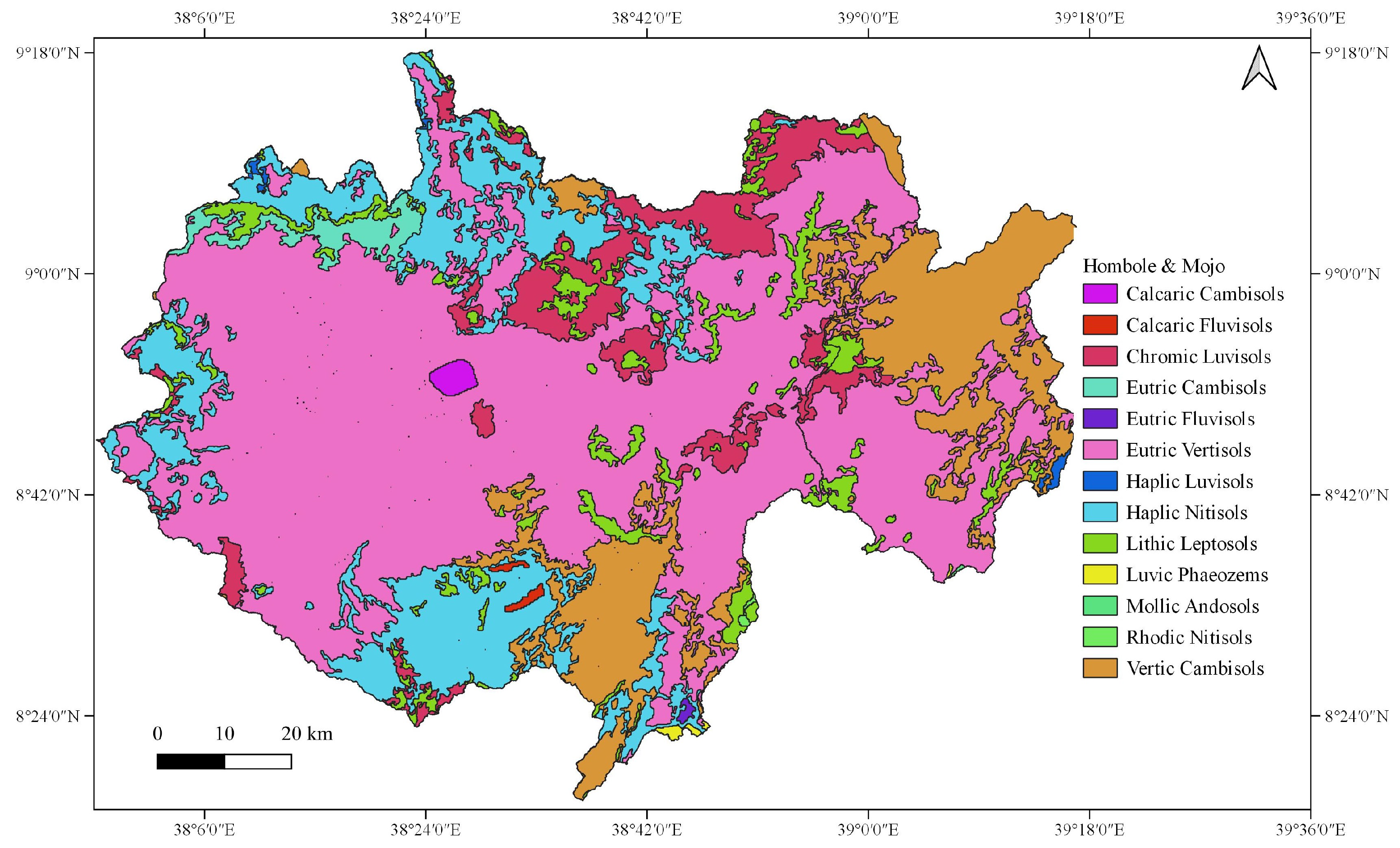
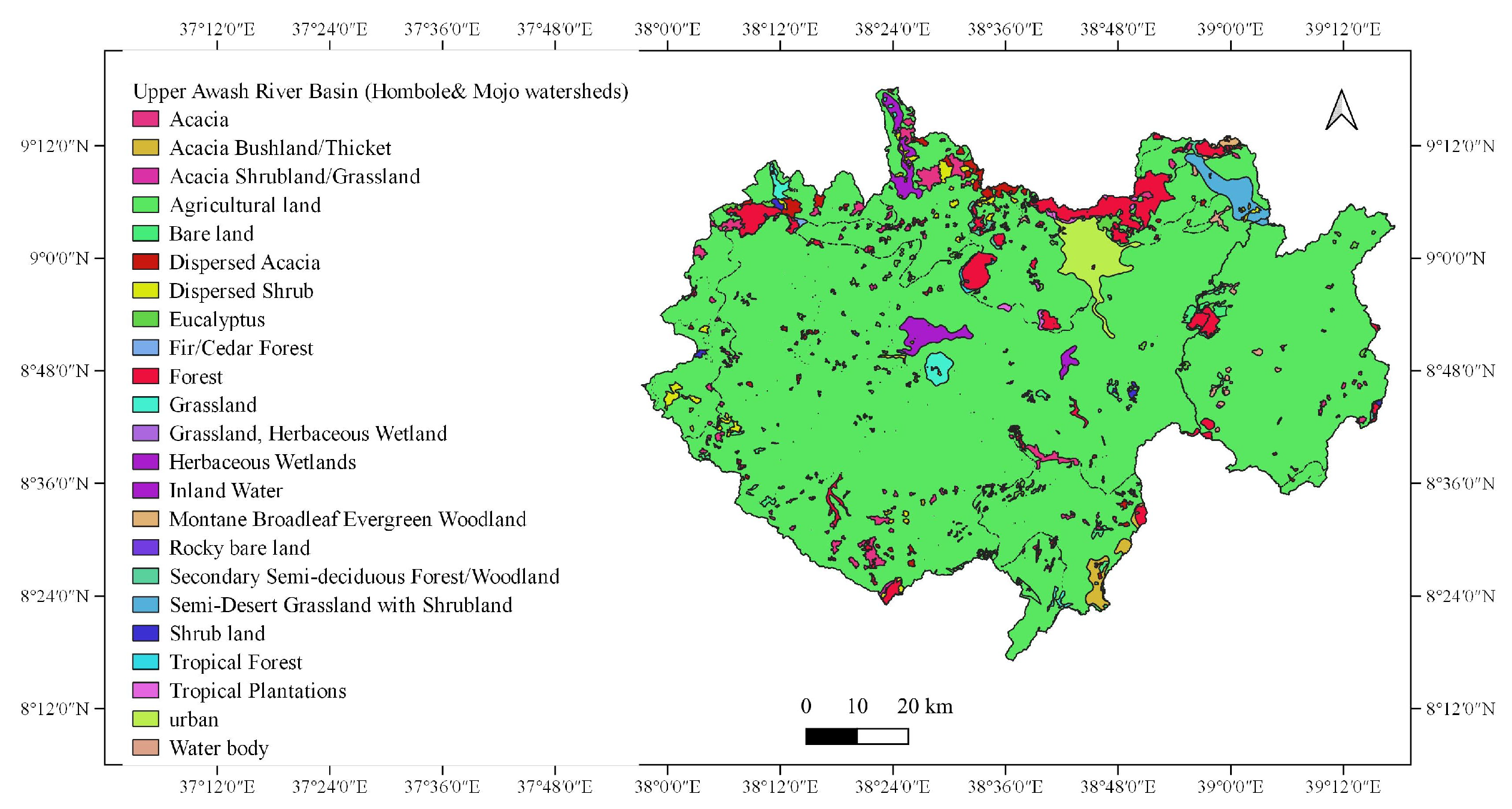
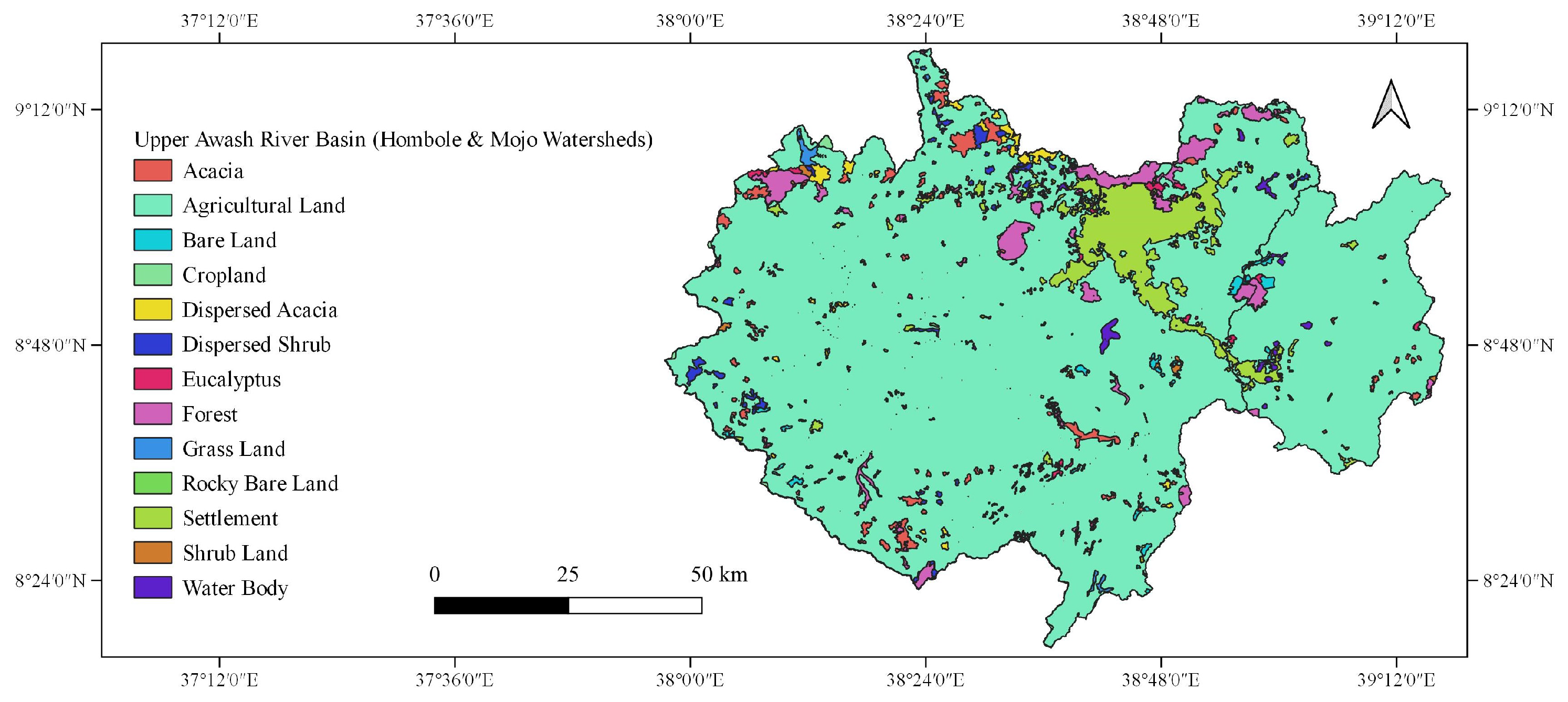
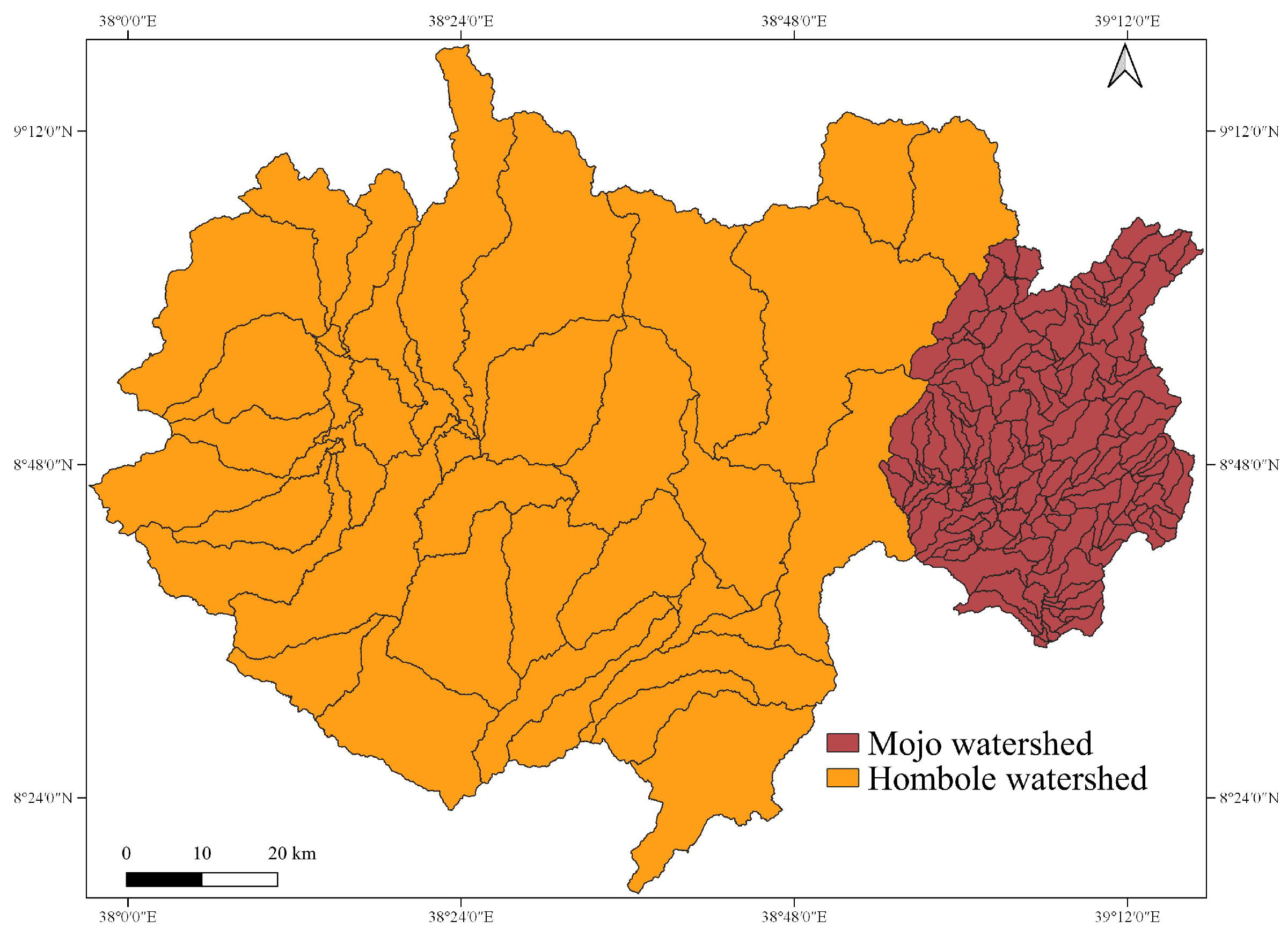
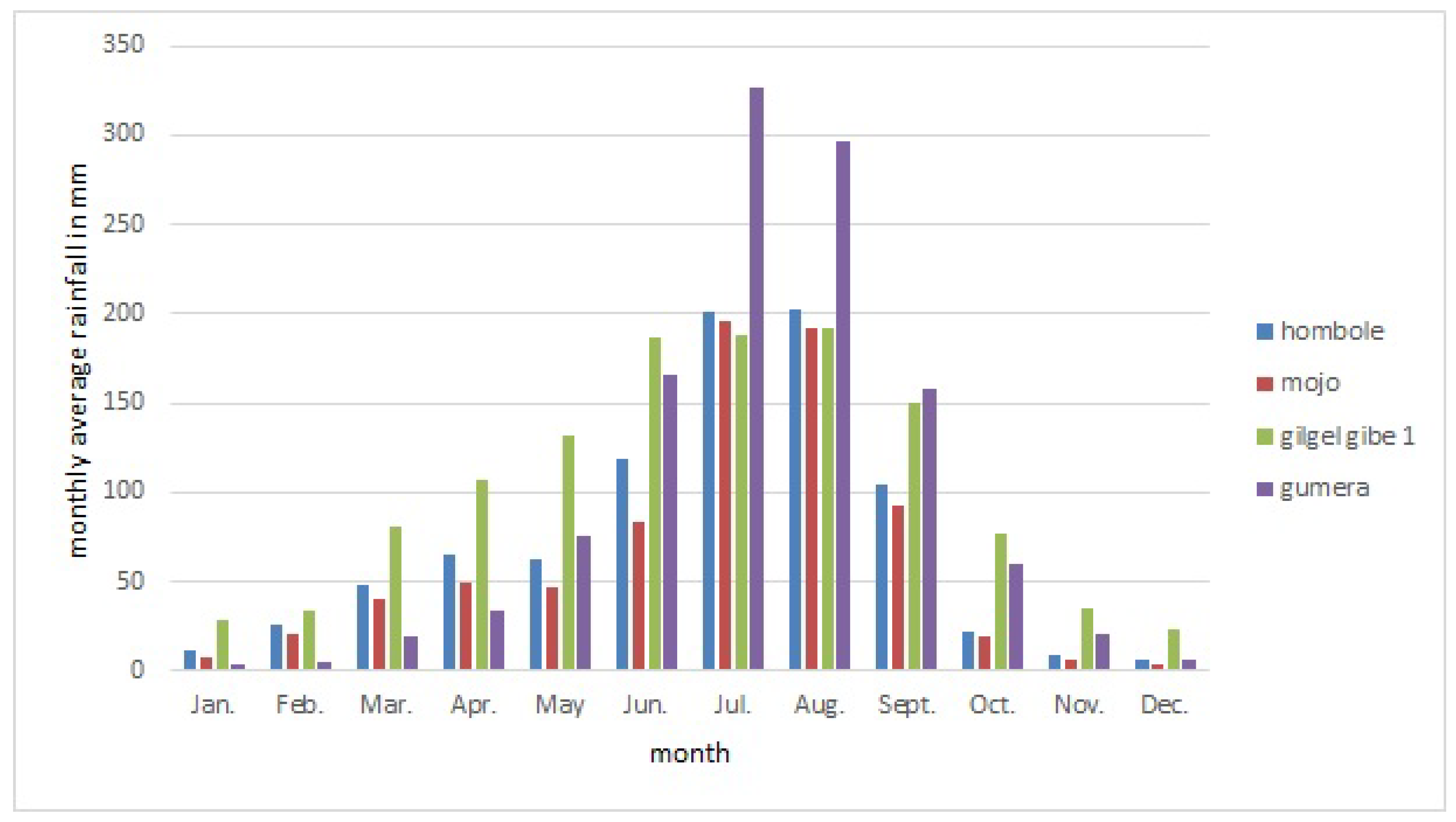
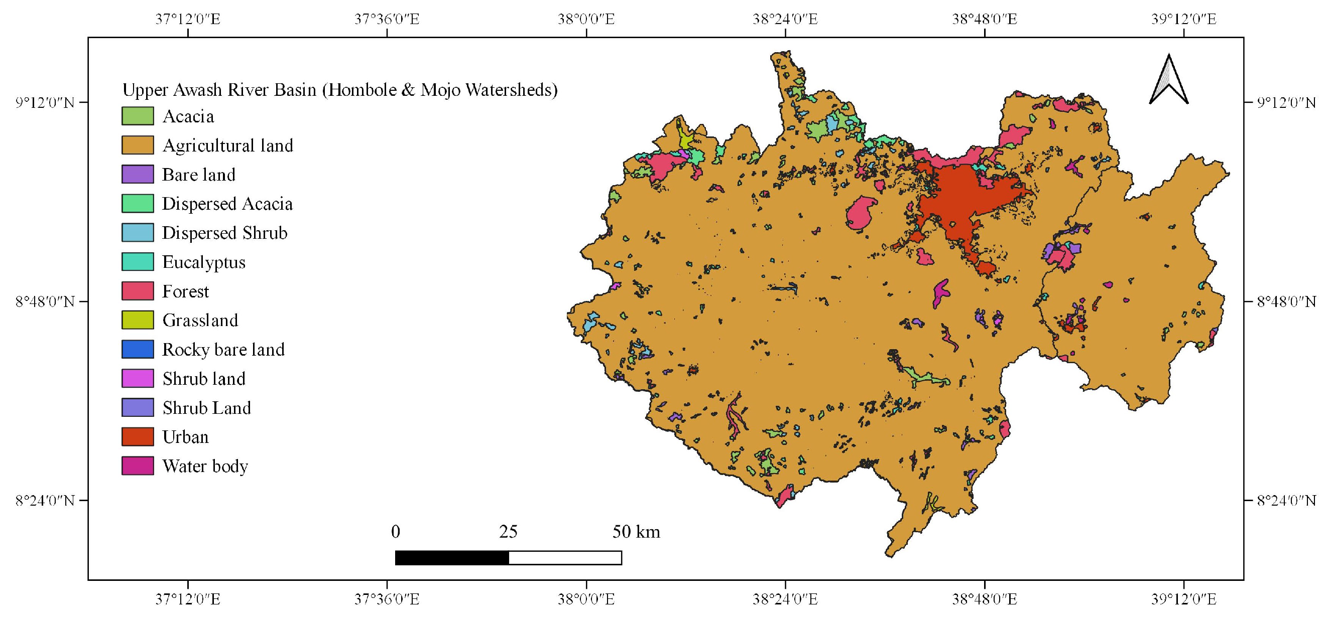
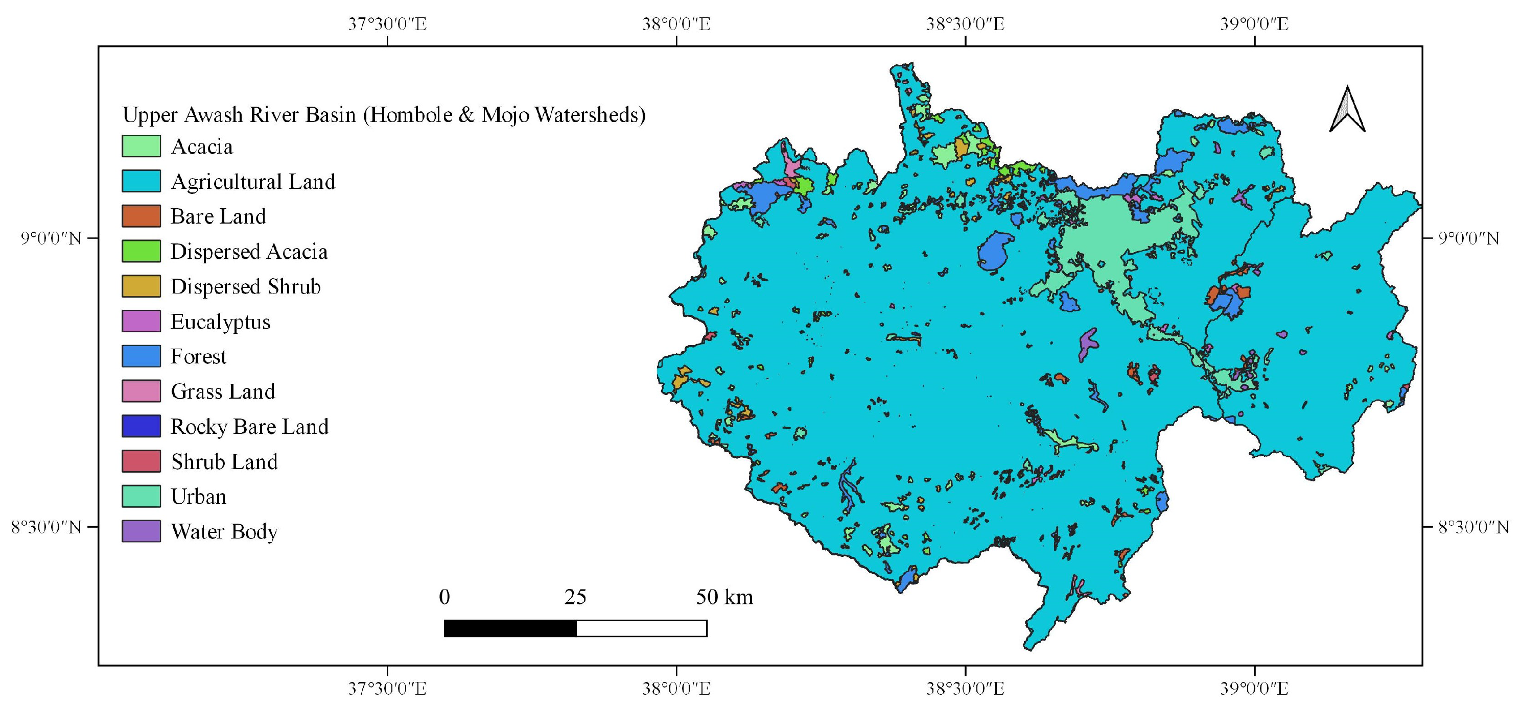
2.1.1. Upper Awash River Basin

The Upper Awash River Basin drains into the Koka hydroelectric power reservoir. The basin comprises two main gauged watersheds: the Hombole and Mojo watersheds, which cover 65.26% and 12.87% of the total area of the basin, respectively. The basin also includes an ungauged watershed which covers 21.87% of the total area of the basin. The total drainage area of the basin is estimated to be 11,680.25 km2.
In the basin, there are active socioeconomic activities like agricultural, industrial, and commercial activities. On the other angle, the basin experienced catastrophic flooding and land degradation problems due to severe gully erosion. The gully erosion assessment in the basin was reported in [12].
For the Hombole and Mojo watersheds (see Figure 1), the monthly average rainfall and monthly average outflow discharge at the main outlet point of the watershed are given in Figure 2 and Figure 3, respectively. The annual average maximum and minimum temperatures were 25.56 °C and 10.06 °C, respectively. The dominant soil types of the watersheds are given in Figure A1. Land use changes were observed in the watersheds, as shown in Figure A4, Figure A5, Figure A6 and Figure A7.

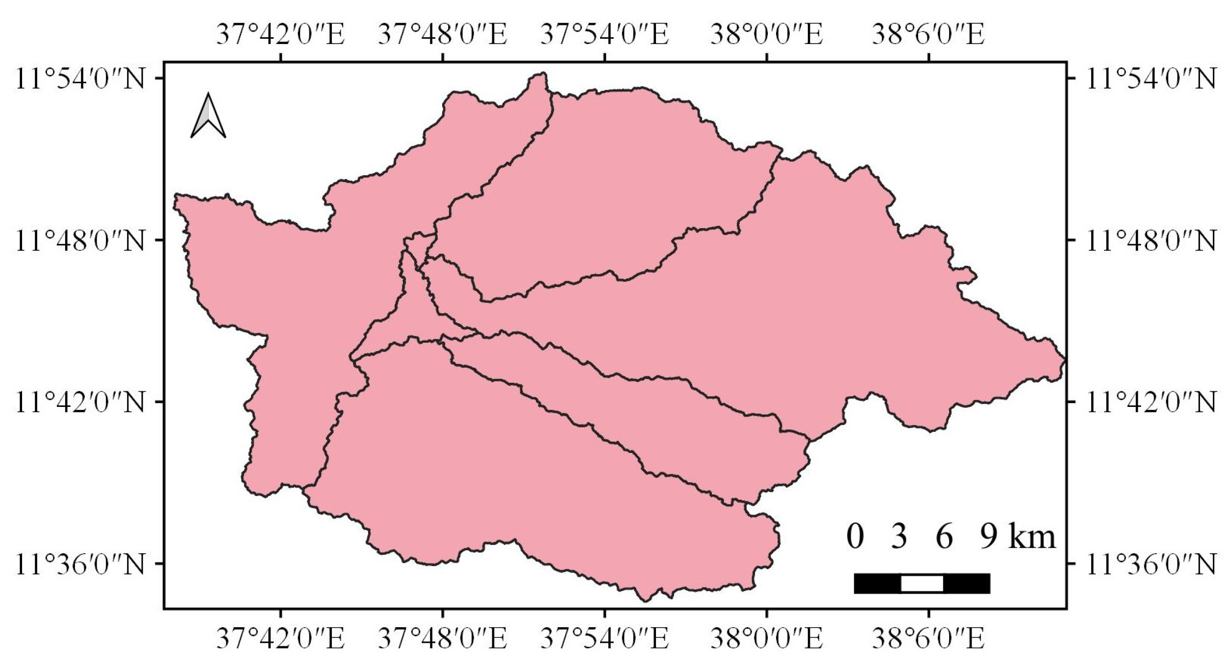
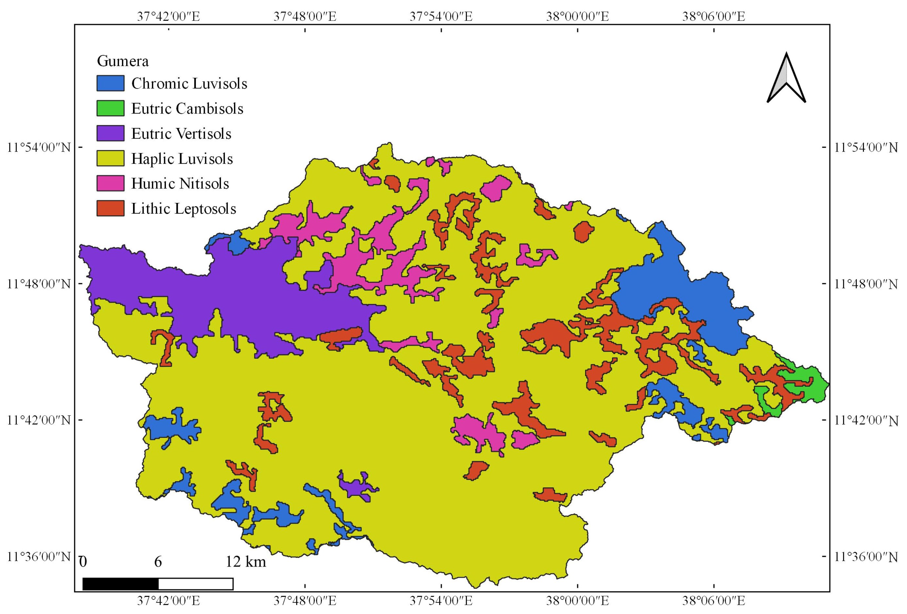
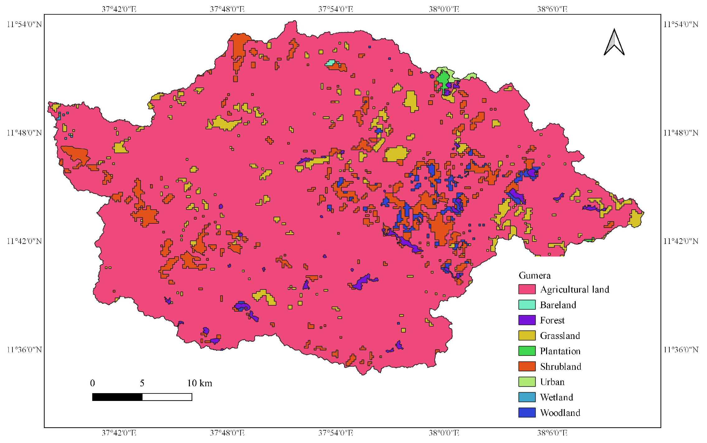
2.1.2. Gumera Watershed

The Gumera Watershed drains into Lake Tana. Its geographic boundary is given in Figure 4. The total drainage area of the watershed is estimated to be 1278.05 km2.
The monthly average rainfall and monthly average outflow discharge at the main outlet point of the watershed are given in Figure 2 and Figure 3, respectively. The annual average maximum and minimum temperatures were 25.38 °C and 10.02 °C, respectively. The dominant soil types of the watershed are given in Figure A2. Land use changes were observed in the watershed, as shown in Figure A8 and Figure A9.

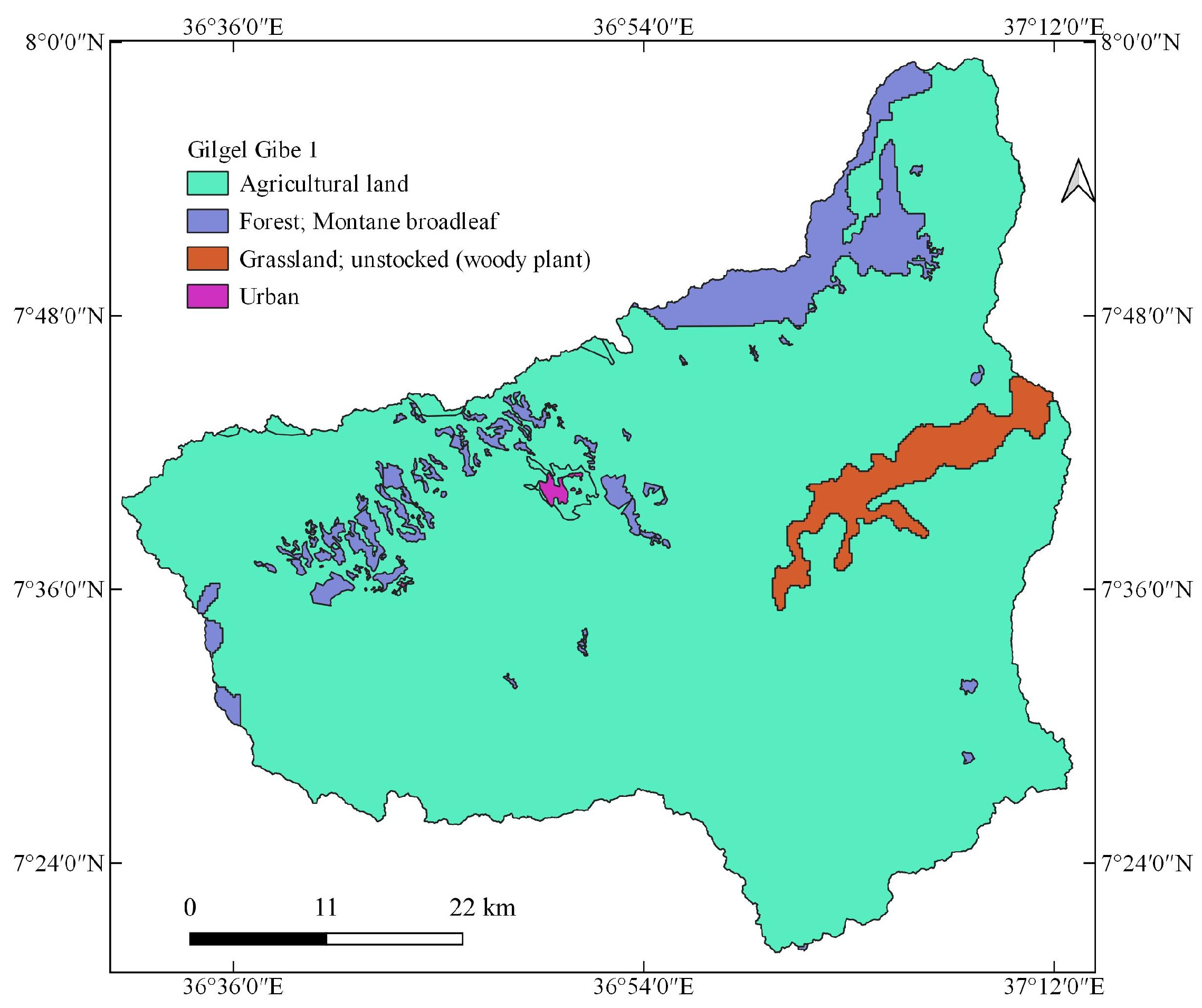
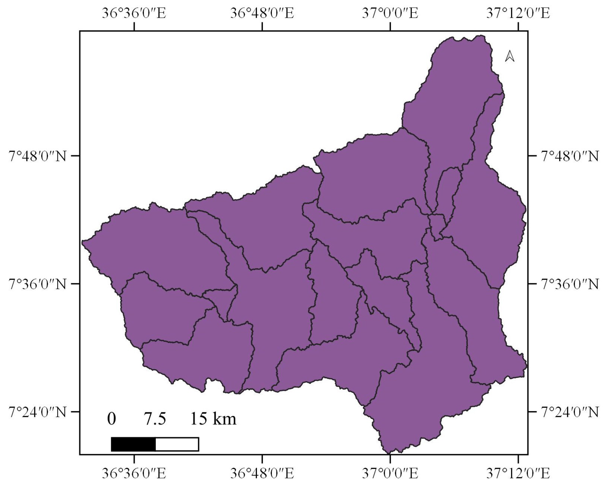
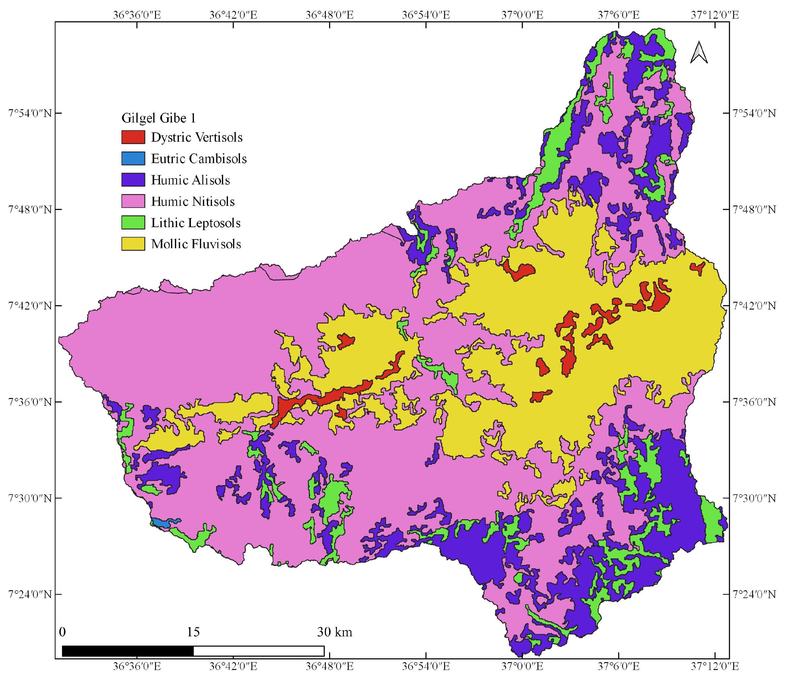
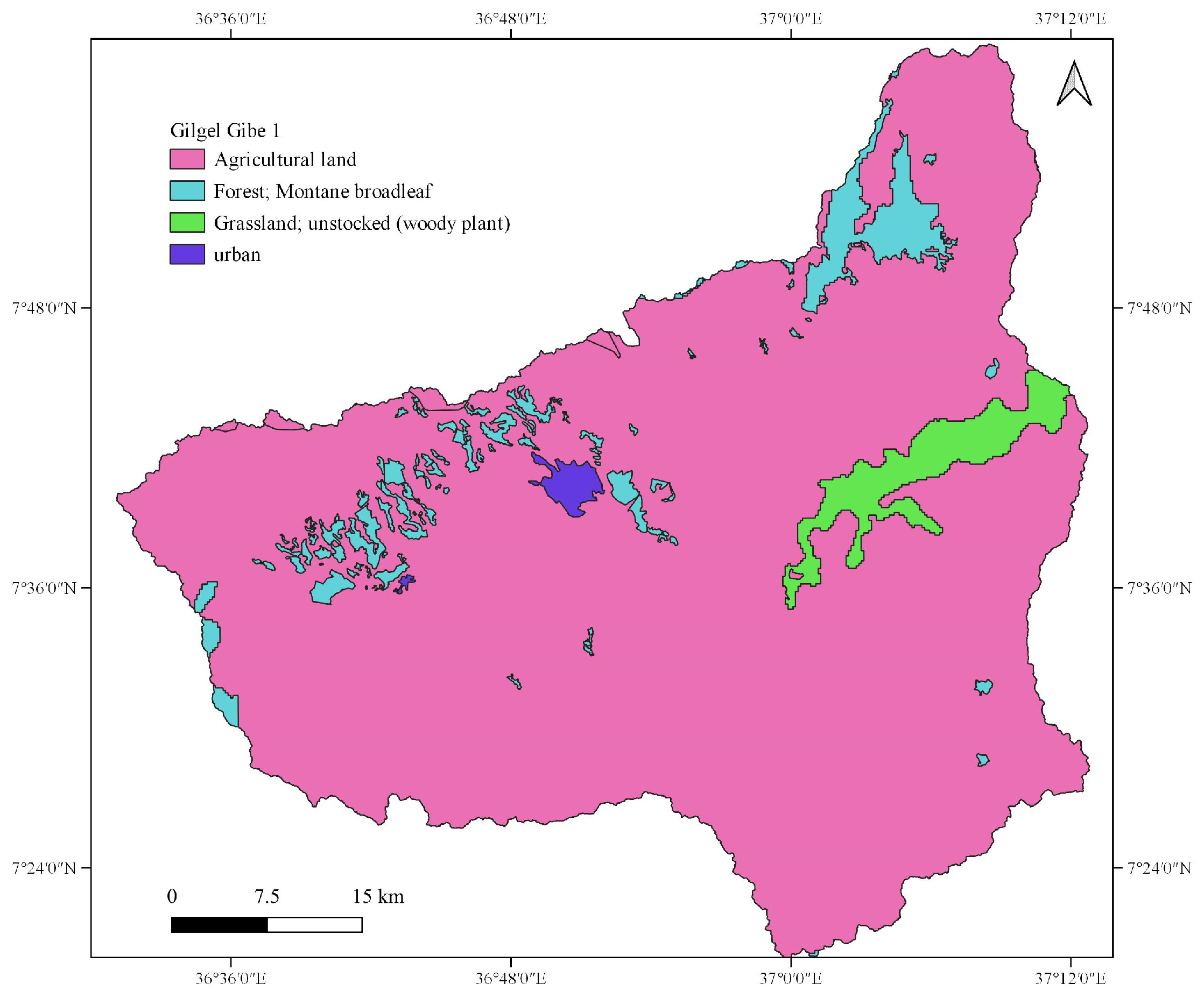
2.1.3. Gilgel Gibe 1 Watershed

The Gilgel Gibe 1 Watershed drains into the Gilgel Gibe 1 hydroelectric power reservoir. Its geographic boundary is given in Figure 5. The total drainage area of the watershed is estimated to be 2928.09 km2.
The monthly average rainfall and monthly average outflow discharge at the main outlet point of the watershed are given in Figure 2 and Figure 3, respectively. The annual average maximum and minimum temperatures were 25.36 °C and 11.7 °C, respectively. The dominant soil types of the watershed are given in Figure A3. Land use changes were observed in the watershed, as shown in Figure A10 and Figure A11.

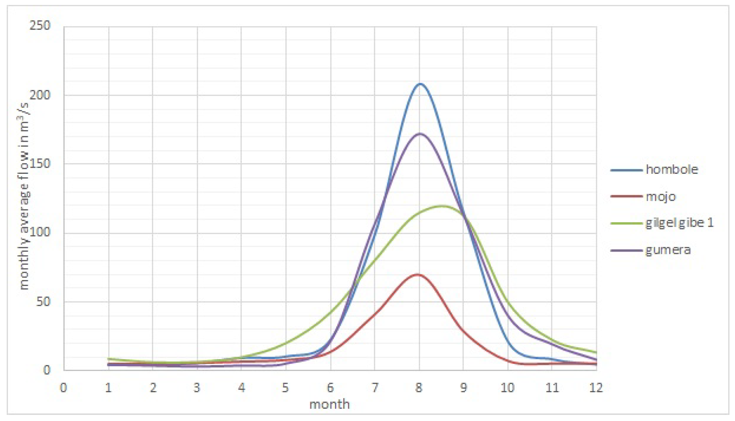
2.2. Sediment Rating Curves

A sediment rating curve was required to generate sediment data from the corresponding flow data. The linear regression equation and nonlinear regression equations such as the power function and the second- and third-order polynomial function could be used to model the sediment rating curve (e.g., [15]). Different authors indicated that the power function is a commonly used nonlinear regression approach to model the sediment rating curve (e.g., [16,17,18]). The power function is given by
C = a Q b
where C is the suspended sediment load or concentration, Q is the discharge, a is the coefficient, and b is the exponent. Different authors reviewed the physical meanings associated with the coefficient a and the exponent b (e.g., [16,19,20]). Accordingly, the coefficient a represents an index of soil erodibility, whereas the exponent b is considered an index of the erosivity and transport capacity of a river. Thus, the power function can be derived by interpreting or deducting the Modified Universal Soil Loss Equation (MUSLE), where its topographic, soil erodibility, cover, and conservation practice factors describe a site-specific condition of a given watershed, and these factors affect the coefficient a of the power function at defined hydroclimatic conditions.
For the sake of simplicity of the regression analysis, the nonlinear regression equation (in our case, the power function) could be transformed into a simple linear regression equation by log transforming both sides of the nonlinear equation accordingly:
l o g ( C ) = l o g ( a ) + b l o g ( Q )
If y = l o g ( C ) , d = l o g ( a ) and x = l o g ( Q ) then , y = b x + d
The Least Squares, Reduced Major Axis Line (RMAL), or other regression methods can be applied to find the best fit regression line on logarithms of suspended sediment load or concentration and discharge data, as well as the back transform of the linear equation results in the power function. Despite there being no generally accepted procedures to model the sediment rating curve, we proceeded with the least squares regression method, which is based on the minimum sum of the squared errors to estimate the coefficient b and the constant d of the best fit linear regression equation for logarithms of the suspended sediment concentration and discharge data:
b = i = 1 n ( x i x ¯ ) ( y i y ¯ ) i = 1 n ( x i x ¯ ) 2
d = y ¯ b x ¯
Aside from choosing the sediment load discharge [21], logged mean loads within discharge classes [20], or sediment concentration discharge [15] approaches, correction factors ( y = C F a Q b ) (e.g., [17,20]) and a power function with some additive constant could be used ([17,22]) to improve the sediment rating curve. Additionally, to improve the sediment rating curve, we may check the data consistency or use a homogeneity test in order to find out the data classes in specific hydroclimatic conditions.
While considering the above advantages and limitations to modeling the sediment rating curve, the relationship between the discharge and suspended sediment concentration rate was checked against the land use change, seasonal weather variations or rainfall pattern, and period of land tillage. Accordingly, the sediment rating curve was drawn while considering the rainfall and discharge relationship for the Gilgel Gibe 1 Watershed, showing some improvement provided that one extreme discharge of 319.65 m3 s−1 on 23 August 2009 (no alike record in the daily average discharge from 1990 to 2015), which corresponded to a suspended sediment concentration of 0.53 kg m−3, was removed from the records as part of the data quality check. In addition, some data replication was possible for improving the sediment rating curve due to the assumption that two measurements that were taken at very small time differences were almost the same, as we only considered a pattern of the record rather than a period of the record, and the data record also did not show watershed information. Accordingly, the sediment rating curve was drawn for the Gumera Watershed, showing some improvement (the change in the coefficient of determination was from R 2 = 0.324 to R 2 = 0.5091 ). For the Hombole and Mojo watersheds, the sediment rating curves were drawn without any preconditions. This was because the above preconditions did not work for these two watersheds. For the Mojo Watershed, two inconsistent records of the rainfall (extremely large and small), flow, and sediment on 7 August 1996 and 6 August 2003 were removed from the records as part of the data quality check. The sediment rating curves of all watersheds are given in Figure 6.

3. Improving MUSLE

The assumption of the USLE and RUSLE is that the rainfall intensity is uniformly distributed over a slope field area. Likewise, in the case of the MUSLE, the runoff is uniformly distributed over the slope field area. The total runoff volume is considered for sediment yield modeling. In both cases, the slope length represents the worst condition for the maximum erosion case, and therefore, the slope length is the shortest distance from the origin of the runoff to the bottom of the slope. The underlying physical assumption to improve the MUSLE is that the amount of potential energy of the runoff is proportional to the shear stress for sediment transport from a slope field and the kinetic energy of the runoff at the bottom of the slope field for gully formation. The potential energy of an object due to its position is given by
P E = m g h = ρ v g h
where P E is the potential energy, m is the mass of the object, g is the acceleration due to gravity, h is the height referring to the position of the object from a reference point, ρ is the density of the object, and v is the volume of the object.
In the process of all of the rainfall in the slope field area, the total potential energy of the runoff is given by [23]
P E = ρ g 4 B L 2 sin 2 θ Q
where P E is the total potential energy of the runoff (J), ρ is the density of water (kg m−3), g is the acceleration due to gravity (m s−2), B is the slope width (m), L is the slope length (m), θ is the slope angle, and Q is the runoff volume (m).
Equation (1) can be applied when the runoff volume flows down from the top of the slope field to the bottom of the slope field, and a temporal variation of the runoff volume is considered. However, this equation does not consider every other runoff volume that will begin at every slope height and flows down simultaneously to the bottom of the slope (i.e., the runoff that will start from any point on the entire slope surface due to the uniform distribution of rainfall on the entire slope field), and it also does not consider a temporal variation of every other runoff volume. Therefore, let us assume that every runoff volume due to raindrops on the entire slope length flows down to the bottom of the slope. Let us say the position of first runoff volume, as well as those of the second, third, and so on along the length of the slope are at the slope heights h, h 1 , h 2 , and so on from the bottom of the slope, respectively. One runoff volume takes over the position of another runoff volume as it flows down to the bottom of the slope.
The total potential energy of the first runoff volume due to its changes in position as it flows down from the height h to the bottom of the slope is equal to E 1 :
E 1 = 0 h ρ v g h d h
The total potential energy of the second runoff volume due to its changes in position as it flows down from the height h 1 (let us say just immediately after the first runoff volume) to the bottom of the slope is equal to E 2 :
E 2 = 0 h 1 ρ v g h d h
The total potential energy of the third runoff volume due to its changes in position as it flows down from the height h 2 (let us say just immediately after the second runoff volume) to the bottom of the slope is equal to E 3 , and so on:
E 3 = 0 h 2 ρ v g h d h
Therefore, the total potential energy of all runoff volumes due to their change in position along the length of the slope to the bottom of the slope is equal to E t :
E t = E 1 + E 2 + E 3 + + E n
Then, we can substitute Equations (2)–(4) into Equation (5):
E t = 0 h ρ v g h d h + 0 h 1 ρ v g h d h + 0 h 2 ρ v g h d h + + E n
0 h ρ v g h d h + 0 h 1 ρ v g h d h + 0 h 2 ρ v g h d h + + E n = 0 h ρ v g h d h d h
where h 1 and h 2 are the heights of the slope just immediately after heights h and h 1 , respectively, and so on:
E t = 0 h ρ v g h d h d h
Each runoff volume ( d v ) in a very small area ( d A ) changes in time ( d t ) with the rainfall intensity ( i r a i n ) and soil infiltration rate ( i s o i l ):
d v = h r u n o f f d A
where h r u n o f f is the runoff depth:
h r u n o f f = ( i r a i n i s o i l ) d t
Then, we can substitute Equation (10) into Equation (9):
d v = ( i r a i n i s o i l ) d t d A
It is noteworthy that only the depth of the runoff volume changed with a small change in time. If it rained continuously for some duration of time, then the runoff volume increased at every point of the slope length. Therefore, the total runoff volume at a particular point of the slope field is a function of the runoff depth changing with time, where the bottom area of the runoff volume does not change with time:
v = d v = 0 t ( d A ( i r a i n i s o i l ) ) d t
Substituting Equation (12) into Equation (8) yields
E t = 0 h ρ g h 0 t ( d A ( i r a i n i s o i l ) ) d t d h d h
For our case, the total potential energy per a unit area ( e t ) is important parameter for soil erosion and sediment transport along the length of the slope, and therefore
e t = E t d A
Substituting Equation (13) into Equation (14) yields
e t = 0 h ρ g h 0 t ( d A ( i r a i n i s o i l ) ) d t d h d h d A
The bottom area of each runoff volume is constant, and therefore
0 t ( d A ( i r a i n i s o i l ) ) d t = d A 0 t ( i r a i n i s o i l ) d t = d A Q
where Q is the runoff volume in m.
Substituting Equation (16) into Equation (15) yields
e t = 0 h ρ g h ( d A Q ) d h d h d A
We can evaluate the integral as follows:
e t = Q ρ g h 3 6
The trigonometric relationship between the slope length, slope angle, and height is given by
h = L sin θ
Substituting Equation (19) into Equation (18) yields
e t = Q ρ g ( L sin θ ) 3 6
We should note that as every runoff volume flows down simultaneously to the bottom of the slope, the runoff concentrates at the bottom of the slope, and it is proportional to the rainfall intensity. The runoff concentration leads to gully formation at the bottom of the slope. The total potential energy of the runoff is proportional to the rainfall intensity.
We can compare the total potential energy of the runoff per unit area (Equation (20)) with the MUSLE:
Q ρ g ( L sin θ ) 3 6 a ( Q q ) b K L S C P
From the relationship in Equation (21), we can reveal the following.
In the MUSLE, a ( Q q ) b L S is the term which contributes to the energy of the runoff, whereas K, C, and P are the coefficients which contribute to the energy dissipation (i.e., K, C and P can be taken as friction resistances against the flow, and the values of K, C, and P vary from 0–1).
Therefore, we can use Q ρ g ( L sin θ ) 3 6 in place of a ( Q q ) b L S in the MUSLE:
y Q ρ g ( L sin θ ) 3 K C P 6
For a given watershed, the topography does not change over time (i.e., the slope length (L) and slope angle ( θ ) are constant). Therefore, the energy of the runoff is proportional to the sediment yield by defining the proportionality constants:
y = a Q b ρ g ( L sin θ ) 3 K C P 6
If the topographic factor of the MUSLE is considered, then
L S ρ g ( L sin θ ) 3 6
where ρ g 6 is the constant.
Therefore, we can use L S in place of ρ g ( L sin θ ) 3 6 in Equation (23):
y = a Q b K L S C P
Therefore, we call Equation (25) the improved MUSLE.

3.1. Estimating the Theoretical Exponent of the Improved MUSLE

As we discussed in the Introduction, the yearly simulation time step is preferred to address the gradual processes of soil erosion and sediment transport. It is important to prove whether a change in the simulation time step changes the coefficient and the exponent of the improved MUSLE or not. This approach led us to estimate the theoretical exponent of the improved MUSLE.
Proof. 
If we consider the small simulation time step and the small simulation period, we can maintain the temporal variation of the factors which directly affect the soil erosion process. For a given field, no change in the cover, conservation practice, or soil erodibility factors of the improved MUSLE will be expected in the small simulation period. At the end of the simulation period, only variation of the coefficient and the exponent of the improved MUSLE with the simulation time step affects the sediment yield output (see the proof steps below for a change in the runoff volume (Q) and the peak runoff rate (q)). If the variations of the coefficient and the exponent of the improved MUSLE with a small change in the simulation time step are detected, then the variations of the coefficient and the exponent with any other simulation time step are confirmed. For the sake of the start, let us consider 1 and 2 unit simulation time steps and a 2-unit simulation period. No change in the factors of the improved MUSLE will be expected for about a 2-unit simulation period. Therefore, the soil loss from a field at the 1-unit simulation time step for about a 2-unit simulation period is equal to the sum of the soil loss at the end of the first and next 1-unit time:
a 1 ( Q 1 ) b 1 K L S C P + a 1 ( Q 2 ) b 1 K L S C P
where suffixes 1 and 2 correspond to the runoff volume (Q), indicating the first and second simulation at the 1-unit simulation time step or interval. It is noteworthy that K , L , S , C , and P are the same for the 2-unit simulation period. The coefficient and the exponent are the same at the 1-unit simulation time step. □
The soil loss from the field at the 2-unit simulation time step for about a 2-unit simulation period is expressed as
a 2 ( Q 1 + Q 2 ) b 2 K L S C P
where a 2 and b 2 indicate a value of the coefficient (a) and exponent (b) at the 2-unit simulation time step. It is noteworthy that the total runoff volume (Q) at the end of the 2-unit simulation period is equal to the sum of the runoff volumes at the end of the first and next 1-unit time.
In either case, the sediment yield is the same, and therefore
a 1 ( Q 1 ) b 1 K L S C P + a 1 ( Q 2 ) b 1 K L S C P = a 2 ( Q 1 + Q 2 ) b 2 K L S C P
a 1 ( Q 1 ) b 1 + a 1 ( Q 2 ) b 1 = a 2 ( Q 1 + Q 2 ) b 2
If there is no variation in the coefficient or exponent with small variation in the simulation time step, then
a 1 = a 2 = a and b 1 = b 2 = b
( Q 1 ) b + ( Q 2 ) b = ( Q 1 + Q 2 ) b
Equation (26) is false if b > 1 or b < 1 . In this case, the coefficient and the exponent of the improved MUSLE change with a change in the simulation time step for a given total simulation period. Equation (26) holds true when b = 1 . This implies that we consider the total runoff volume per storm event (i.e., from the beginning of runoff to the end of the runoff from a slope field) to estimate the total sediment load. The objective of the improved MUSLE is to estimate the total sediment load transported from the beginning of runoff to the end of the runoff from the slope field. Therefore, the theoretical exponent of the improved MUSLE is one. It is a theoretical exponent because the left and right sides of Equation (26) represent the theoretical linked expressions without knowledge of the observed sediment. With knowledge of the observed sediment, the actual exponent of the improved MUSLE can be obtained by applying the model at the selected watersheds of Ethiopia.

3.2. Estimating the Factors of the Improved MUSLE

The improved MUSLE shares the same factors with the USLE, RUSLE, and MUSLE. The original factors of the USLE represent the average value for estimating the annual sediment yield. The unit plot [8] represents the worst case for the maximum soil erosion in a given rainfall event. It is practically impossible to directly measure each field slope, slope length, the temporal variation of soil erodibility, instantaneous runoff, cover change, and conservation practice for a large watershed. In the actual field, the field slope and length are not uniform, which means they are irregular. The topographic, soil erodibility, cover, and conservation practice factors depend on the spatial resolution of the digital elevation model (DEM) and soil and land use maps, respectively. Therefore, in the actual sediment modeling, the average field slope length [24] and slope steepness, or simply the topographic factor [25], average runoff, average soil erodibility factor [26], and average cover and conservation practice factors, are taken.

3.2.1. Estimation of Runoff Factor

In the MUSLE, the runoff factor is the product of the total runoff volume and peak runoff rate. In the improved MUSLE, the peak runoff rate is eliminated. To estimate the runoff factor of the improved MUSLE, the volume of the runoff can be obtained by direct measurement of the runoff on a storm event basis and also by using indirect methods such as the Soil Conservation Service Curve Number (SCS CN) method, rational method, flood routing, or unit hydrograph. For our case, we used the daily average discharge to estimate the annual total runoff volume for the annual sediment yield estimation. The reasons for why we used directly measured flow data and why we estimated the annual sediment yield are addressed in the Introduction.

3.2.2. Estimation of Soil Erodibility Factor (K-Factor)

The authors in [8] defined the soil erodibility factor as the soil loss rate per erosion index unit for a specified soil as measured on a unit plot. The unit plot is defined as a 72.6 feet in length uniform 9% slope continuous in a clean-tilled fallow. It is the continuous fallow that is tilled up and down the slope. The soil erodibility factor is given by [8]
K = n = 1 N A n n = 1 N E I 30 n
where A is the event soil loss from the unit plot in t o n s a c r e 1 y e a r 1 , E is the storm kinetic energy in 100 ∗ foot-tons per acre, I 30 is the maximum 30-min intensity in inches per hour, and K is the soil erodibility factor in 0.01 t o n s a c r e h o u r a c r e 1 y e a r 1 f o o t 1 t o n s 1 i n c h 1 . It is important to note that the soil erodibility factor represents the worst or the maximum possible erosion from the unit plot with the specified field slope and length. At the same rainfall impact pressure, a lesser soil erosion condition that is different from the worst condition takes into account the soil cover and conservation practice on the same field slope and length. On the unit plot, or any unit plot for that matter, the temporal and spatial variation of the soil erodibility depend on the type of soil and the quite complex interaction of physical, biological, chemical, and mechanical processes. From the soil erodibility table or equations, we can reveal that the soil erodibility factor varies from 0 to 1, where 0 indicates the soil that is hard to erode, whereas 1 represents easily erodible soil under the same rainfall impact pressure in otherwise similar soil erosion conditions. From this range of the soil erodibility factor, we can conclude that soil erodibility refers to the degree of ease in eroding a given soil.
The soil erodibility factor (K-factor) can be estimated by direct field measurement or by using different empirical equations or a soil erodibility nomograph:
  • The K-factor that was originally developed in the soil conditions of the USA [8]:
    K = 2.1 M 1.14 10 4 12 a + 3.25 b 2 + 2.5 c 3 100
    where K = soil erodibility in 0.01 t o n s a c r e h o u r a c r e 1 y e a r 1 f o o t 1 t o n s 1 i n c h 1 , M = ( % s i l t + % v e r y f i n e s a n d ) ( 100 % c l a y ) , M = the particle size parameter, silt (%) = the percentage of silt, % very fine sand = the percentage of very fine sand (0.1–0.05 mm), clay (%) = the percentage of clay, a = the percentage of organic matter, b = the soil structure code used in soil classification, and c = the profile permeability class. For soils containing less than 70 percent silt and very fine sand, the nomograph [8] is used to solve the above equation.
    To comment on this equation, we did not have a percentage of very fine sand in our database to test the equation. Our source of data was the harmonized world soil data, which includes the texture, reference soil depth, drainage class, available water capacity, sand, silt and clay fractions, bulk density, gravel content, organic carbon content, pH, cation exchange capacity, base saturation, total exchangeable bases, calcium carbonate content, gypsum content, sodicity, and salinity content. As land tillage and mechanical compaction (due to rainfall impact) change the structure of the soil, the structure of the tilled, bare, or compacted soil varies at the temporal and spatial scales. As soil permeability depends on the soil texture and organic matter, their relationship should be explicitly shown. Unrealistic values were obtained for tropical soils from the equation’s erodibility nomograph (Mulengera and Payton, 1999; Ndomba, 2007), as cited in [6].
  • The K-factor (Williams and Renard, 1983) as cited in [27] and with a similar equation in [28,29]:
    K = ( 0.2 + 0.3 exp ( 0.0256 S a ( 1 s i 100 ) ) ) ( S i c L + s i ) 0.3 ( 1 0.25 c c + exp ( 3.72 2.95 c ) ) ( 1 0.7 S N S N + exp ( 5.51 + 22.9 S N ) )
    where S a = sand (%), S i = silt (%), C L = clay (%), S N = 1 ( S a / 100 ) , and C = organic carbon.
  • The K-factor that was tested in the soil conditions of the Philippines [30]:
    K = 0.043 p H + 0.62 O M + 0.0082 S 0.0062 C S i
    where p H = the pH of the soil, O M = organic matter (%), S = the sand content (%), C = the clay ratio = % clay/(% sand + % silt), and S i = silt content = % silt/100.
  • The K-factor that was originally developed in the volcanic soil of Hawaii, USA (El-Swaify and Dangler, 1976) as cited in [31]:
    K = 0.03970 + 0.00311 x 1 + 0.00043 x 2 + 0.00185 x 3 + 0.00258 x 4 0.00823 x 5
    where x 1 is the unstable aggregate size fraction (<0.250 mm) in percent, x 2 = modified silt (0.002–0.1 mm) (%) ∗ modified sand (0.1–2 mm) (%), x 3 = % base saturation, x 4 is the silt fraction (0.002–0.050 mm) (%), and x 5 is the modified sand fraction (0.1–2 mm) (%).
    We did not have an unstable aggregate size fraction or modified silt and sand data in our database to test the equation.
  • Williams (1995) proposed the following K-factor, as cited in [32]:
    K = f c s a n d f c l s i f o r g C f h i s a n d
    f c s a n d = 0.2 + 0.3 exp [ 0.256 m s ( 1 m s i l t 100 ) ]
    f c l s i = ( m s i l t m c m s i l t ) 0.3
    f o r g C = 1 0.25 o r g C o r g C + exp [ 3.72 2.95 o r g C ]
    f h i s a n d = 1 0.7 ( 1 m s 100 ) 1 m s 100 + exp [ 5.51 + 22.9 ( 1 m s 100 ) ]
  • Other soil erodibility equations are mentioned in [29,31,32,33,34,35,36,37].
The procedure to test the above soil erodibility equations on the basis of the original definition of the soil erodibility are given in [1]. According to the procedure, we used Williams’s (1995) equation as cited in [32] to calculate the soil erodibility factor using the soil data of the watersheds under our consideration: the watersheds of Ethiopia in general.

3.2.3. Estimation of the Slope Steepness and Slope Length Factors

The slope steepness factor (S) is the ratio of soil loss from a field slope gradient to the soil loss from the 9% slope under otherwise identical conditions [38]. A high rate of soil loss is associated with steep slopes [26,39], and soil loss prediction is more sensitive to the slope steepness than slope length [40].
The slope length is defined as the distance from the point of origin of overland flow to the point where either the slope gradient decreases enough that deposition begins or the runoff water enters a well-defined channel that may be part of a drainage network or a constructed channel [8]. It is important to note that the definition of the slope length relies on the conditions at which the unit plot was constructed according to [8]. The unit plot represents the worst condition for the maximum soil erosion case. Therefore, for the worst condition for the maximum erosion case, the slope length is the shortest distance from the origin of the overland flow to the point where deposition takes place or enters the stream channels. The slope lengths would rarely have a constant gradient along their entire length, and the slope irregularities would affect the amount of soil movement to the foot of the slope [8]. The slope length factor is given by [8]:
L = λ λ 0 m
where λ is the slope length, λ 0 is the unit plot length of 72.6 ft = 22.13 m, and λ 0 is also defined as the horizontal projection of the slope length (e.g., [39,41,42,43]). In one term, the slope steepness factor (S) and slope length factor (L) together is called the topographic factor (LS factor). The topographic factor is the ratio of soil loss per unit area from a field slope length and gradient to that from the 22.1-m length of a uniform 9% slope under otherwise identical conditions [8]. Different equations have been suggested at different locations to estimate the topographic factor while taking into account site-specific conditions:
  • The topographic factor that was proposed for the topographic conditions in the USA [8]:
    L S = ( λ 72.6 ) m ( 65.41 sin 2 θ + 4.56 sin θ + 0.065 )
    where λ = the slope length in feet, θ = the angle of the slope, and m is dependent on the slope (0.5 if slope >5%, 0.4 if slope is between 3.5% and 4.5%, 0.3 if slope is between 1% and 3%, and 0.2 if slope is less than 1%).
  • McCool et al. (1987) improved the LS factor from the classic USLE for use in terrain with steeper slopes, as cited in [25], for use in the RUSLE [39]:
    L = λ 22.13 m
    m = sin θ sin θ + 0.269 sin θ 0.8 + 0.05
    S = 3.0 sin θ 0.8 + 0.56 f o r λ < 4 m
    S = 10.8 sin θ + 0.03 f o r λ > 4 m a n d s < 9 %
    S = 16.8 sin θ 0.50 f o r λ > 4 m a n d s > 9 %
    where λ is the slope length in meters, m is the dimensionless parameter, θ is the angle of the field slope in degrees (tan-1 (s/100)), and s is the field slope as a percentage.
  • Foster et al. (1977) and McCool et al. (1987, 1989) proposed the following equations for the calculation of the LS factors, as cited in [31]:
    • L = λ 72.6 m ;
    • m = β 1 + β (Foster et al., 1977), as cited in [31];
    • β = sin θ 0.0896 3.0 sin θ 0.8 + 0.56 (McCool et al., 1989), as cited in [31];
    • S = 10.8 sin θ + 0.03 if the slope (s) is less than 9% (McCool et al., 1987), as cited in [31];
    • s = 16.8 sin θ 0.5 if the slope is greater than or equal to 9% ( McCool et al., 1987), as cited in [31].
    • S = 3.0 sin θ 0.8 + 0.56 if the slope length is shorter than 4.6 m (McCool et al., 1987), as cited in [31], for the condition where water drains freely from the slope end, and it is assumed that inter-rill erosion is insignificant on slopes shorter than 4.6 m [39]. Here, λ is the slope length (ft), θ is the angle of the slope, and m is dependent on the slope (0.5 if slope > 5%, 0.4 if the slope is between 3.5% and 4.5%, 0.3 if the slope is between 1% and 3%, and 0.2 if the slope is less than 1%). As a remark, when the conditions favor more inter-rill and less rill erosion, as in the cases of consolidated soils like those found in no-till agriculture, m should be decreased by halving the β value, where a low rill to inter-rill erosion ratio is typical of the conditions in rangelands [39]. With thawing and cultivated soils dominated by surface flow, a constant value of 0.5 should be used (McCool et al., 1989, 1993), as cited in [39]. When freshly tilled soil was thawing, in a weakened state, and primarily subjected to surface flow, we used the following (McCool et al., 1993), as cited in [39]:
      S = 10.8 sin θ + 0.03 s < 9 %
      S = sin θ 0.0896 0.6 s > 9 %
    • The slope factor which is approximately equal to the LS factor in the topographic conditions of the Philippines [30]:
      S = a + b S L 4 / 3
      where S is the slope factor, a = 0.1, b = 0.21, and S L is the slope in percent.
  • The LS factor was developed in the topographic conditions of Britain [44]:
    L S = λ 22 0.50 0.065 + 0.045 s + 0.0065 s 2
    where λ is the slope length (m) and s is the slope steepness (%).
  • Apart from the LS factor of the USLE and RUSLE, the Chinese Soil Loss Equation [45] was developed while taking into consideration the Chinese soil environment and topographic conditions (including the modified equation that can calculate the LS factor in >10° conditions) [46]. In the Chinese soil loss equation, the LS factor is calculated by [46]
    L = λ 22.1 m
    m = 0.2 f o r θ 1.7 %
    m = 0.3 f o r 1.7 % < θ 5.2 %
    m = 0.4 f o r 5.2 % < θ 9 %
    m = 0.5 f o r θ > 9 %
    S = 10.8 sin θ + 0.03 f o r θ < 9 %
    S = 16.8 sin θ 0.05 f o r 9 % θ < 17.6 %
    S = 21.9 sin θ 0.96 f o r θ 17.6 %
    where λ is the slope length (m), m is the variable slope length exponent, and θ is the slope angle (°).
  • Other equations for the slope or slope length factor are mentioned in [25,40,45,46,47,48,49].
To estimate the topographic factor (LS) for our watersheds, SWATplus was used to define as many hydrologic response units (hrus) as possible to consider an areal distribution of the slope steepness and slope length. In the TxtInOut folder of SWATplus, the area and topography information of each hru were stored in the hru and topography files, respectively. These files were exported to an Excel spreadsheet for analysis. The area, slope, and slope length of each hru were used to estimate the LS factor for each hru by using the above equations and Equations (27) and (28), stated below. The weighted average of the LS factors was taken to represent the watershed. The best fit methods were chosen during calibration of the annual sediment yield (see the calibration stage below).

3.2.4. Estimation of the Cover Factor (C Factor)

This is the ratio of soil loss from a field with specified cropping to that from a clean-tilled continuous fallow under otherwise similar conditions. These similar conditions are no soil conservation works (land is tilled up and down the slope) and the soil, slope steepness, slope length, and rainfall impact pressure being the same for both the cropped field and fallow area. The C factor is related to land use and land cover, and it is the reduction factor to soil erosion vulnerability [50]. Therefore, the C factor lies between 0 and 1, which describes the extent of vegetation cover to protect the soil from erosion in a given catchment. Its value being closer to zero indicates dense vegetation cover, whereas its value being closer to one indicates poor vegetation cover. Essentially, the surface cover or canopy protects from soil erosion by decreasing the rainfall impact energy, but it may have less importance in protecting sediment transport from a field. To some extent, we can say that the surface cover affects soil erosion by reducing the transport capacity of the runoff water (Foster, 1982) and by causing deposition in ponded areas (Laflen, 1983), as cited in [31], and also by decreasing the surface area susceptible to raindrop impacts [31]. In addition, the plant root depth and distribution as well as the porosity increase the infiltration rate of rainfall water into the soil, and thus they play a role in reducing soil loss (Jeong et al. 2012), as cited in [51].
Although the C factor value can be taken from the literature or determined in situ, an extensive literature review compiling the potential soil loss rates of different crop and forest covers compared to the likely soil loss rates of bare soil can be used to determine the likely C factor values of a particular site [48]. The published guidelines [8,39], the revised C factor (Cai et al., 2000) as cited in [52], and the Normalized Difference Vegetation Index [36,37] can be used to compute the C factor. For our case, the annual or average annual cover factor for each land use category was adopted based on the assessment of the literature. The authors in [48] reviewed the C factors for the general types of land use and land cover. For our watersheds, the adopted cover factor for each land use is shown in Table 1. To estimate an areal weighted average of the cover factor for our watersheds, SWATplus was used to define as many hydrologic response units (hru) as possible to consider the areal distributions of land use and land cover. In the TxtInOut folder of SWATplus, the area of each hru is stored in the hru file, and the hru’s land use data files are stored in the hru data file. These files are exported to an Excel spreadsheet for analysis and calculation of the areal weighted average. We can use the shapefile of each land use map (see Figure A4, Figure A5, Figure A6, Figure A7, Figure A8, Figure A9, Figure A10 and Figure A11) to estimate the areal coverage of each land use class in QGIS, and then the corresponding C and P factors can be assigned.

3.2.5. Estimation of Soil Conservation or Erosion Control Practice Factor (P-Factor)

This is the ratio of soil loss associated with a specific support practice in the corresponding soil loss when cultivation is performed up and down the slope [31] under otherwise similar conditions. The P factor describes the effects of practices such as contouring, strip cropping, concave slopes, terraces, grass hedges, silt fences, straw bales, and subsurface drainage [50]. These conservation practices change the direction and speed of runoff [39]. It mainly reduces the transport of soil particles by blocking runoff and breaking its speed, but it does not reduce rainfall impact energy to reduce soil erosion. Therefore, the P factor ranges from 0 to 1, where 0 represents strong conservation practice (no soil loss from a field is expected) and 1 represents the worst conditions for maximum erosion due to a lack of conservation practice and when the land is tilled up and down the slope such that runoff takes the shortest well-defined channel or route in the field.
The difficulty of accurately mapping support practice factors or not observing support practices leads to many studies ignoring this by giving their P factor a value of 1.0 [48]. Some P factors can be ignored if some C factors already account for the presence of a support factor such as intercropping or contouring [48]. All non-agricultural lands were also assigned a value of one if no feasible conservation measures were applied [26,51,52]. At suitably detailed scales, and with enough knowledge of farming practices, using the P factor may lead to a more accurate estimation of soil loss [48]. The authors in [4] revealed that considering the temporal variation of the P factor could significantly improve the performance of the MUSLE, although it has been rarely taken into account. The soil conservation or erosion control practice factors can be estimated with the help of available tables [8], using land use and land cover maps [26,51,52], and through field measurement (see the literature review report in [4]). For our case, the annual soil conservation practice factor for each land use category is adopted based on the assessment of the literature. The authors in [48] reviewed the P factors for general types of land use and land cover. The adopted P factor for the land use and land cover category of each watershed is shown in Table 1. The areal weighted average of the P factor was found in the same manner as the cover factor.

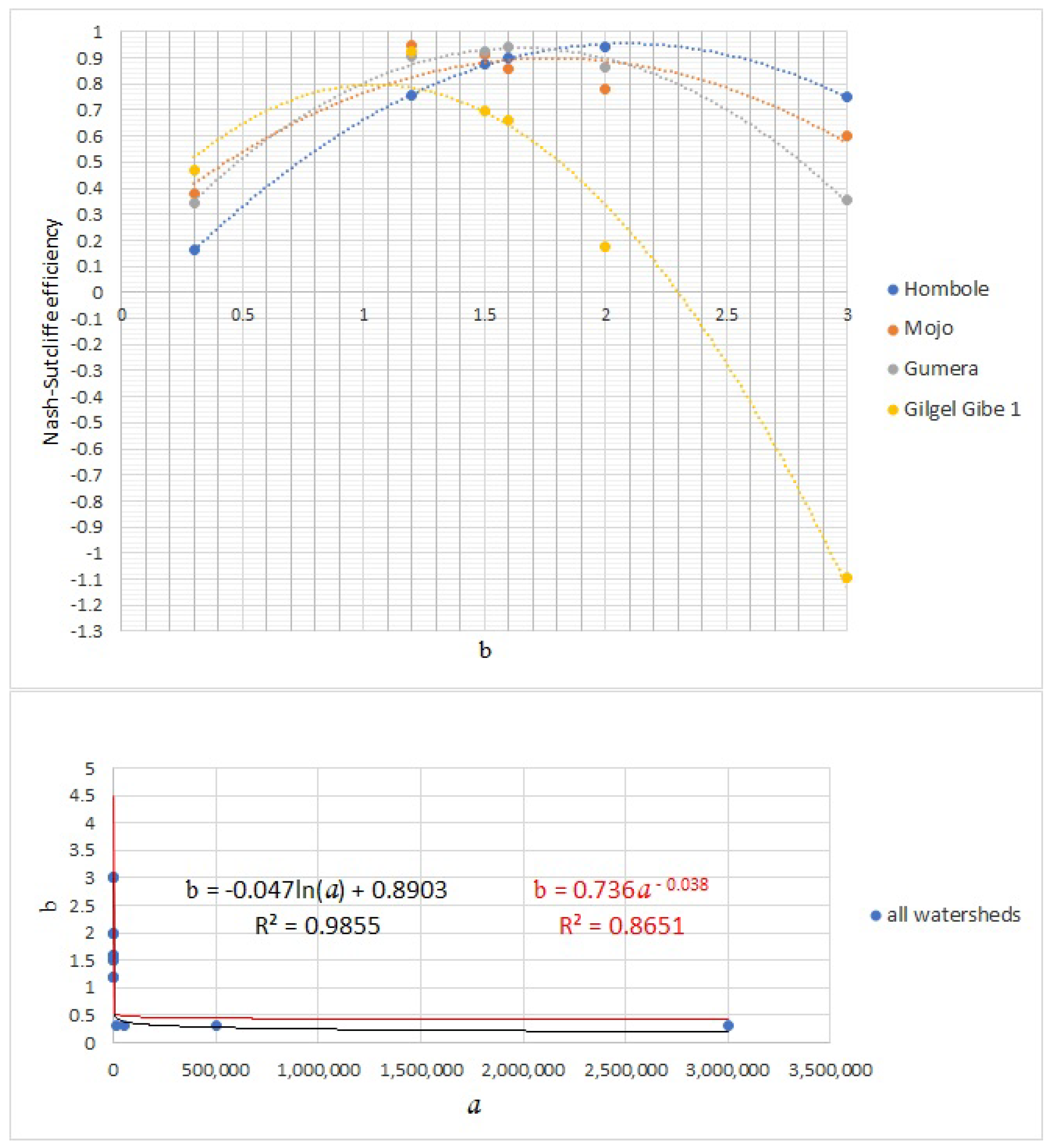
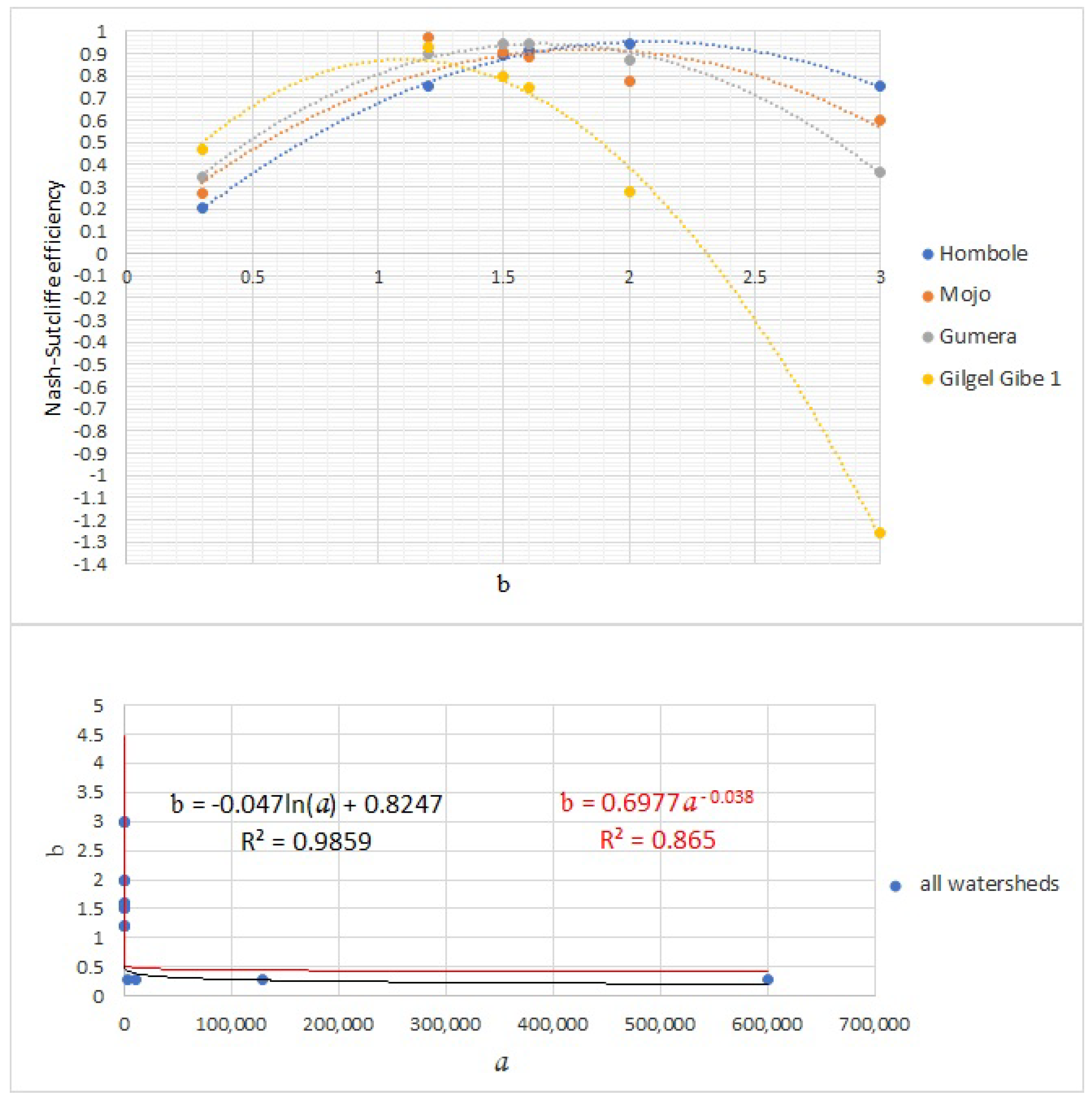
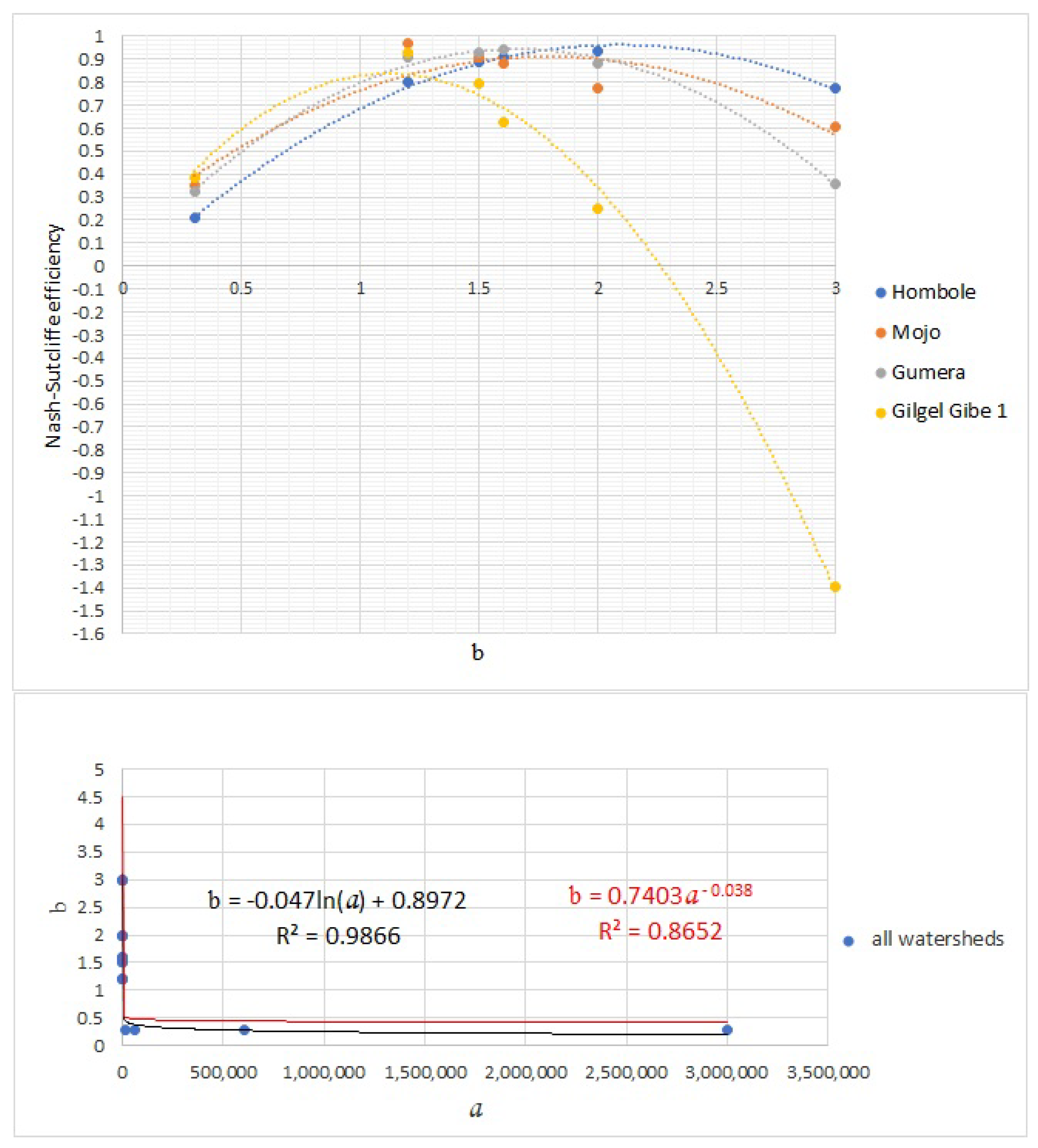
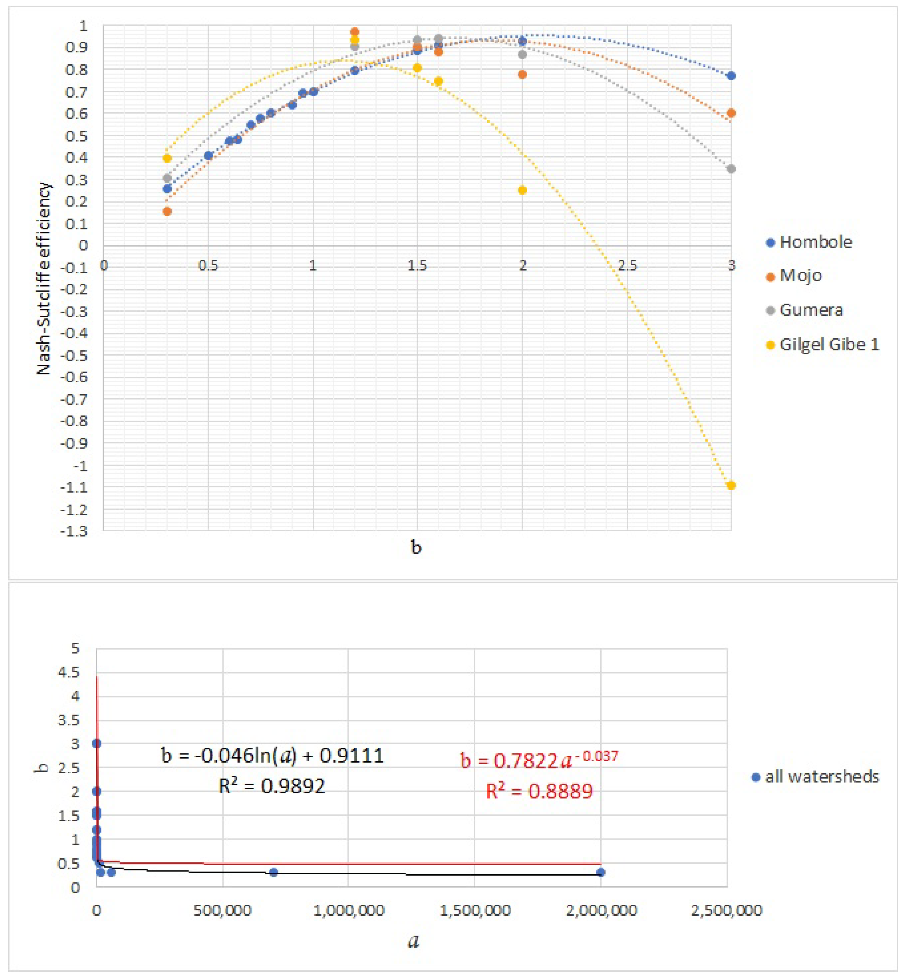
3.2.6. Estimation of Coefficient a and Exponent b through Calibration
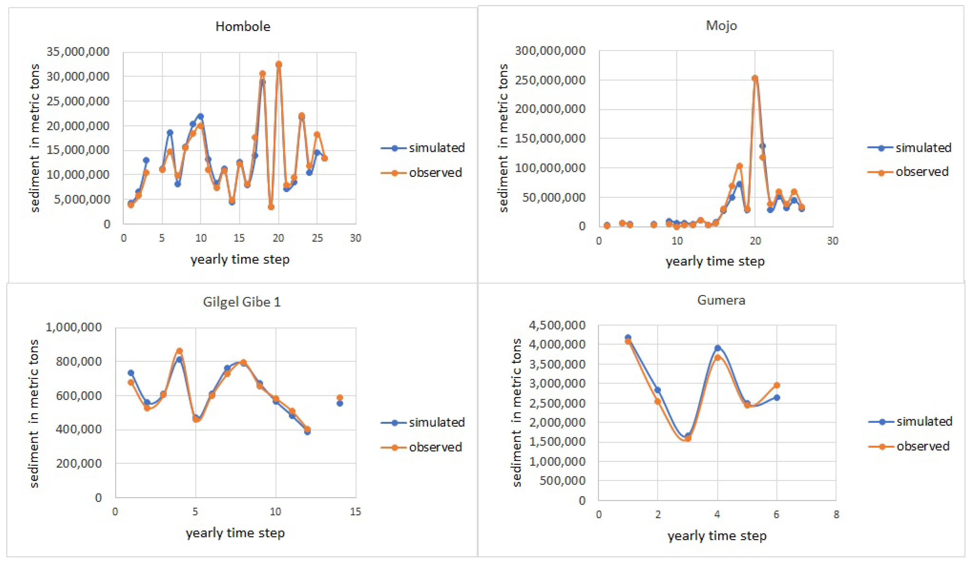
For a chosen value of the exponent b, the best fit corresponding value of coefficient a was estimated through calibration. The selection of the best exponent and the best equation among those listed above and below (see Equations (27) and (28)) for the topographic factor was performed after calibration of the observed and simulated sediment (i.e., the improved MUSLE was used to estimate the sediment load). Figure 7 shows sample graphs of the calibrated sediment when the topographic factor was calculated using the equation that was proposed in [8].
During calibration, the Nash–Sutcliffe efficiency corresponds to each LS factor, exponent b and coefficient a are evaluated, and graphs of exponent b versus the Nash–Sutcliffe efficiency and coefficient a versus exponent b are drawn for each watershed, as shown in Figure 8, Figure 9, Figure 10, Figure 11, Figure 12, Figure 13 and Figure 14. For a chosen value of b, we tested seven different equations of the topographic factor for each watershed. Therefore, we could have as many graphs as possible.
L S = ( 0.02222 J 1.5 + 0.03231 J + 0.1004 ) 0.2901 y 0.4002 f o r J < 5 %
L S = ( 0.02222 J 1.5 + 0.03231 J + 0.1004 ) 0.2105 y 0.5004 f o r J > 5 %
where J is the slope in percent and y is the slope length. For a description, readers are encouraged to watch the video at https://www.youtube.com/watch?v=w6w8jxbTJfo (accessed on 25 February 2021). For the case of the watersheds under our consideration, we took △y/22.1 as the field slope length.

4. Results

We called Equation (25) the improved MUSLE. The input data requirement of the MUSLE was changed for calculation of its runoff factor, for possible application of the model using only the runoff volume, and the topographic, soil erodibility, cover, and conservation practice factors. From all graphs (see Figure 8, Figure 9, Figure 10, Figure 11, Figure 12, Figure 13 and Figure 14), the best actual exponent b of the improved MUSLE was 1.2, which resulted in a Nash–Sutcliffe efficiency of approximately 1 irrespective of the topographic factor, whereas the theoretical exponent of the improved MUSLE was 1. Therefore, the best exponent of the improved MUSLE was obtained only through calibration of the observed and simulated sediment.
From all the graphs (see Figure 8, Figure 9, Figure 10, Figure 11, Figure 12, Figure 13 and Figure 14), if we considered one watershed, we took the exponent and topographic factor which resulted in the maximum Nash–Sutcliffe efficiency, but if we considered two or more watersheds, we took the exponent and topographic factor which resulted in the minimum Nash–Sutcliffe efficiency. Accordingly, the best exponent of the improved MUSLE was 1.3, which resulted in a Nash–Sutcliffe efficiency of approximately 0.84 if the topographic factor was calculated by using the equation that was proposed in [31]. Therefore, this was the best combination of the exponent and topographic factor of the improved MUSLE under the hydroclimatic conditions of all watersheds under our consideration. Compared with the original MUSLE [1], the improved MUSLE showed better performance (i.e., the minimum performance was 84%) over the original MUSLE (i.e., the minimum performance was 80%).
To find the best combination of the exponent and topographic factor, the important relationships between coefficient a and exponent b as well as exponent b and the Nash–Sutcliffe efficiency were drawn for future evaluation of the improved MUSLE at any watershed. As we can see from the graphs (see Figure 8, Figure 9, Figure 10, Figure 11, Figure 12, Figure 13 and Figure 14), for the observed and simulated sediment, as the relationship between coefficient a and exponent b approached the power or logarithmic function, the relationship between exponent b and the Nash–Sutcliffe efficiency approached a quadratic function. This relationship can be used to find the best performance of the improved MUSLE during calibration of the model.

5. Discussion

To improve the MUSLE, we assumed that the amount of potential energy of the runoff was proportional to the shear stress for sediment transport from a slope field and the kinetic energy of the runoff at the bottom of the slope field for gully formation. The authors of [23] underestimated the total potential energy of the runoff that would be available for soil erosion and sediment transport (compare Equations (1) and (20)). Based on the physical assumption, the peak runoff rate was eliminated from the variables of the MUSLE. This improvement had an advantage for the possible application of the model in data-scarce areas and not use indirect methods to estimate the peak runoff rate.
To compare the improved MUSLE with the original MUSLE, we followed a similar evaluation procedure to evaluate the improved MUSLE versus the original MUSLE. The evaluation procedure for the original MUSLE is discussed in [1]. The improved MUSLE showed better performance (i.e., the minimum performance was 84%) over the original MUSLE (i.e., the minimum performance was 80%) for all watersheds under consideration. This improvement may be linked to the uncertainty in the peak runoff rate (i.e., uncertainty in the interpretation of the daily flow data for the yearly peak runoff rate) or other unknown reasons. As all variables of the improved MUSLE are parts of the original MUSLE, there is no indication to say gully erosion is considered in the improved MUSLE, as per the physical assumption that we made to improve the MUSLE.
We used the Williams (1995) equation as cited in [32] to calculate the soil erodibility factor, as we found it to be the best equation for the soil erodibility factor [1]. We considered land use maps to assign a value for the cover and conservation practice factors from past experiences in the literature, and the coefficient a was estimated through calibration. Since only a produced effect of the coefficient, soil erodibility, cover, and conservation practice factors is reflected in the improved MUSLE rather than their individual effects during calibration of the sediment yield, any change in these factors affected the coefficient of the improved MUSLE. Therefore, we do not like suggesting strict procedures to estimate these factors. It is highly preferable that these factors are measured and studied at a temporal and spatial scale to understand their effect on soil erosion in a particular field. This is because the soil erodibility, cover, and conservation practice factors reflect site-specific conditions. For example, we can talk about the density and pattern of land cover, nature and extent of soil conservation and flood protection work, and the temporal variation in soil properties.

6. Conclusions

The improved MUSLE showed better performance (i.e., the minimum performance was 84%) over the original MUSLE (i.e., the minimum performance was 80%) for all four watersheds under consideration. The performance of the improved MUSLE was greater than or equal to 84% for all four watersheds under consideration, provided that the exponent of the model was 1.3, and its topographic factor was calculated by using the equations in [31]. This can be taken as the best combination of the exponent and topographic factor under the hydroclimatic conditions in Ethiopia. We recommend further investigation of the best combination of the exponent and topographic factor by applying the improved MUSLE at different watersheds in Ethiopia.
As per our discussion above, we cannot exactly tell whether gully erosion is considered in the improved MUSLE or not. As part of the comparison between the original MUSLE and the improved MUSLE, what different effect does the peak runoff rate have on soil erosion and sediment transport compared with the runoff volume? As far as the lumped model is concerned, the individual effect of the runoff and peak runoff rate on soil erosion and sediment transport should be explicitly shown. This helps us to put a physical demarcation between the peak runoff rate and runoff volume. Therefore, better explanation and further improvement of the MUSLE may become necessary to address soil erosion and sediment transport problems. In the improved MUSLE (the same for the original MUSLE), the topographic factor is directly proportional to the soil erosion and sediment yield. However, as the slope length becomes larger and larger, there is a possibility that soil erosion from the upper part of the slope gets deposited at the lower part of the slope. Therefore, more research is required to understand the effect of the slope length on soil erosion and sediment transport.
The improved MUSLE considers the topographic factor of the original MUSLE. Equation (23) does not consider the topographic factor of the original MUSLE; therefore, this equation should also be tested.

Author Contributions

This research article is part of PhD research by M.G.T.; major supervisor, A.M.; co-supervisor, Y.S. All authors have read and agreed to the published version of the manuscript.

Funding

This PhD research was funded by the German Academic Exchange Service (91742735): EECBP Home Grown PhD Scholarship Programme and the Universität der Bundeswehr: Scholarship and Support Program for Foreign Students and Doctoral Candidates (STIBET III) Matching Funds Scholarship.

Institutional Review Board Statement

Not applicable.

Informed Consent Statement

Not applicable.

Data Availability Statement

Land use and soil data sources are available at https://www.preprints.org/manuscript/202202.0163/v2 (accessed on 24 March 2022). Climate data (from 1986 to 2020 for all watersheds) are from the National Meteorology Agency of Ethiopia. Flow data (from 1990 to 2016 for Hombole and Mojo watersheds; from 2000 to 2017 for Gumera watershed; from 2000 to 2015 for Gilgel Gibe 1 watershed) and sediment data (from 1989 to 2015 for Hombole and Mojo watersheds; from 1990 to 2017 for Gumera and Gilgel Gibe 1 watersheds) are from the River Basin Authority of Ethiopia. Digital elevation models are from the US Geological Survey.

Acknowledgments

We acknowledge financial support from Universität der Bundeswehr München.

Conflicts of Interest

The authors declare no conflict of interest.

Appendix A

Figure A1. Soil maps of Hombole and Mojo watersheds.
Water 14 01450 g0a1
Figure A2. Soil map of Gumera Watershed.
Water 14 01450 g0a2
Figure A3. Soil map of Gilgel Gibe 1 Watershed.
Water 14 01450 g0a3

Appendix B

Figure A4. Land use map of Upper Awash River Basin (Hombole and Mojo watersheds) from 1989 to 2000.
Water 14 01450 g0a4
Figure A5. Land use map of Upper Awash River Basin (Hombole and Mojo watersheds) from 2001 to 2008.
Water 14 01450 g0a5
Figure A6. Land use map of Upper Awash River Basin (Hombole and Mojo watersheds) from 2009 to 2012.
Water 14 01450 g0a6
Figure A7. Land use map of Upper Awash River Basin (Hombole and Mojo watersheds) from 2013 to 2015.
Water 14 01450 g0a7
Figure A8. Land use map of Gumera Watershed from 1989 to 2009.
Water 14 01450 g0a8
Figure A9. Land use map of Gumera Watershed from 2010 to 2015.
Water 14 01450 g0a9
Figure A10. Land use map of Gilgel Gibe 1 Watershed from 1989 to 2009.
Water 14 01450 g0a10
Figure A11. Land use map of Gilgel Gibe 1 Watershed from 2010 to 2015.
Water 14 01450 g0a11

References

  1. Tsige, M.G.; Malcherek, A.; Seleshi, Y. Estimating the Best Exponent of the Modified Universal Soil Loss Equation and Regionalizing the Modified Universal Soil Loss Equation Under Hydro-climatic Condition of Ethiopia. Preprints 2022, 2022020163. [Google Scholar] [CrossRef]
  2. Williams, J.R. Sediment Routing for Agricultural Watersheds. Water Resour. Bull. 1975, 11, 965–974. [Google Scholar] [CrossRef]
  3. Williams, J.R.; Berndt, H.D. Sediment Yield Prediction Based on Watershed Hydrology. ASAE 1977, 20, 1100–1104. [Google Scholar] [CrossRef]
  4. Sadeghi, S.H.R.; Gholami, L.; Darvishan, A.K.; Saeidi, P. A review of the application of the MUSLE model worldwide. Hydrol. Sci. J. 2014, 59, 365–375. [Google Scholar] [CrossRef] [Green Version]
  5. Sadeghi, S.H.; Mizuyama, T.; Vangah, B.G. Conformity of MUSLE Estimates and Erosion Plot Data for Storm-Wise Sediment Yield Estimation. Terr. Atmos. Ocean. Sci. 2007, 18, 117–128. [Google Scholar] [CrossRef] [Green Version]
  6. Adegede, A.P.; Mbajiorgu, C.C. Event-Based Sediment Yield Modelling Using MUSLE in North-Central Nigeria. Agric. Eng. Int. Cigr J. 2019, 21, 7–17. Available online: https://cigrjournal.org/index.php/Ejounral/article/view/5231 (accessed on 23 January 2020).
  7. Muche, H.; Temesgen, M.; Yimer, F. Soil Loss Prediction Using USLE and MUSLE under Conservation Tillage Integrated with ‘Fanya Juus’ in Choke Mountain, Ethiopia. Int. J. Agric. Sci. 2013, 3, 46–52. Available online: https://internationalscholarsjournals.org/print.php?article=soil-loss-predictionusing (accessed on 10 November 2021).
  8. Wischmeier, W.H.; Smith, D. Predicting Rainfall Erosion Losses: A Guide to Conservation Planning; U.S. Department of Agriculture (USDA): Washington, DC, USA, 1978.
  9. Soil Conservation Service. Geologic Investigation for Watershed Planning; Technical Release No. 17 Geology; USDA: Washington, DC, USA, 1966. Available online: https://directives.sc.egov.usda.gov/OpenNonWebContent.aspx?content=18602.wba (accessed on 23 January 2020).
  10. Amare, S.; Langendoen, E.; Keesstra, S.; van der Ploeg, M.; Gelagay, H.; Lemma, H.; van der Zee, S.E.A.T.M. Susceptibility to Gully Erosion: Applying Random Forest (RF) and Frequency Ratio (FR) Approaches to a Small Catchment in Ethiopia. Water 2021, 13, 216. [Google Scholar] [CrossRef]
  11. Haregeweyn, N.; Tsunekawa, A.; Poesen, J.; Tsubo, M.; Meshesha, D.T.; Fenta, A.A.; Nyssen, J.; Adgo, E. Comprehensive assessment of soil erosion risk for better land use planning in river basins: Case study of the Upper Blue Nile River. Sci. Total Environ. 2017, 574, 95–108. [Google Scholar] [CrossRef] [Green Version]
  12. Kropače, K.J.; Schillaci, C.; Salvini, R.; Maerker, M. Assessment of Gully Erosion in the Upper Awash, Central Ethiopian Highlands Based on a Comparison of Archived Aerial Photographs and Very High Resolution Satellite Images. Geogr. Fis. Dinam. Quat. 2016, 39, 161–170. [Google Scholar]
  13. Frankl, A.; Deckers, J.; Moulaert, L.; Damme, A.V.; Haile, M.; Poesen, J.; Nyssen, J. Integrated Solutions for Combating Gully Erosion in Areas Prone to Soil Piping: Innovations from the Drylands of Northern Ethiopia. Land Degrad. Dev. 2014, 27, 1797–1804. [Google Scholar] [CrossRef]
  14. Haregeweyn, N.; Tsunekawa, A.; Nyssen, J.; Poesen, J.; Tsubo, M.; Meshesha, D.T.; Schutt, B.; Adgo, E.; Tegegne, F. Soil erosion and conservation in Ethiopia: A review. Prog. Phys. Geogr. 2015, 39, 750–774. [Google Scholar] [CrossRef] [Green Version]
  15. Horowitz, A.J. An evaluation of sediment rating curves for estimating suspended sediment concentrations for subsequent flux calculations. Hydrol. Process. 2003, 17, 3387–3409. [Google Scholar] [CrossRef]
  16. Heng, S.; Suetsugi, T. Comparison of regionalization approaches in parameterizing sediment rating curve in ungauged catchments for subsequent instantaneous sediment yield prediction. J. Hydrol. 2014, 512, 240–253. [Google Scholar] [CrossRef]
  17. Asselman, N.E.M. Fitting and interpretation of sediment rating curves. J. Hydrol. 2000, 234, 228–248. [Google Scholar] [CrossRef]
  18. Hapsari, D.; Onishi, T.; Imaizumi, F.; Noda, K.; Senge, M. The Use of Sediment Rating Curve under its Limitations to Estimate the Suspended Load. Rev. Agric. Sci. 2019, 7, 88–101. [Google Scholar] [CrossRef] [Green Version]
  19. Efthimiou, N. The role of sediment rating curve development methodology on river load modeling. Environ. Monit. Assess. 2019, 191, 108. [Google Scholar] [CrossRef]
  20. Talebia, A.; Bahrami, A.; Mardian, M.; Mahjoobi, J. Determination of optimized sediment rating equation and its relationship with physical characteristics of watershed in semiarid regions: A case study of Pol-Doab waters. Desert 2015, 20, 135–144. [Google Scholar] [CrossRef]
  21. Balamurugan, G. The Use of Suspended Sediment Rating Curves In Malaysia: Some Preliminary Considerations. Pertanika 1989, 12, 367–376. [Google Scholar]
  22. Doomen, A.M.C.; Wijma, E.; Zwolsman, J.J.K.; Middelkoop, H. Predicting suspended sediment concentrations in the Meuse River using a supply-based rating curve. Hydrol. Process. 2008, 22, 1846–1856. [Google Scholar] [CrossRef]
  23. Li, G.-L.; Zheng, T.-Z.; Fu, Y.; Li, B.-Q.; Zhang, T. Soil detachment and transport under the combined action of rainfall and runoff energy on shallow overland flow. J. Mt. Sci. 2017, 14, 1373–1383. [Google Scholar] [CrossRef]
  24. Desmet, P.J.J.; Govers, G. A GIS procedure for automatically calculating the USLE LS factor on topographically complex landscape units. J. Soil Water Conserv. 1996, 51, 427–433. [Google Scholar]
  25. Pongsai, S.; Vogt, D.S.; Shrestha, R.P.; Clemente, R.S.; Apisit, E. Calibration and validation of the Modified Universal Soil Loss Equation for estimating sediment yield on sloping plots: A case study in Khun Satan catchment of Northern Thailand. Can. J. Soil Sci. 2010, 90, 585–596. [Google Scholar] [CrossRef] [Green Version]
  26. Gwapedza, D.; Slaughter, A.; Hughes, D.; Mantel, S. Regionalising MUSLE factors for application to a data-scarce catchment. Water Resources Assessment ans Seasonal Prediction. In Proceedings of the International Association of Hydrological Sciences; Copernicus GmbH: Göttingen, Germany, 2018; Volume 377, pp. 19–24. [Google Scholar] [CrossRef] [Green Version]
  27. Chen, L.; Qian, X.; Shi, Y. Critical Area Identification of Potential Soil Loss in a Typical Watershed of the Three Gorges Reservoir Region. Water Resour. Manag. 2011, 25, 3445–3463. [Google Scholar] [CrossRef]
  28. Cole, G.W.; Cooley, K.R.; Dyke, P.T.; Favis-Mortlock, D.T.; Foster, G.R.; Hanson, C.L.; Jones, C.A.; Jones, O.R.; Kiniry, J.R.; Laflen, J.M.; et al. EPIC—Erosion/Productivity Impact Calculator; Technical Bulletin Number 1768; United States Department of Agriculture, Agricultural Research Service: Washington, DC, USA, 1990.
  29. Kruk, E. Use of Chosen Methods for Determination of the USLE Soil Erodibility Factor on the Example of Loess Slope. J. Ecol. Eng. 2021, 22, 151–161. [Google Scholar] [CrossRef]
  30. David, W.P. Soil and Water Conservation Planning: Policy Issues and Recommendations. J. Philipp. Dev. 1988, XV, 47–84. [Google Scholar]
  31. Renard, K.G.; Foster, G.R.; Weesies, G.A.; McCool, D.K.; Yoder, D.C. Predicting Soil Erosion by Water: A Guide to Conservation Planning with the Revised Universal Soil Loss Equation; Agriculture Handbook, No 703; USDA: Washington, DC, USA, 1997; p. 404.
  32. Wawer, R.; Nowocien, E.; Podolski, B. Real and Calculated KUSLE Erodibility Factor for Selected Polish Soils. Pol. J. Environ. Stud. 2005, 14, 655–658. [Google Scholar]
  33. Wischmeier, W.H.; Mannering, J.V. Relation of Soil Properties to its Erodibility. Soil Sci. Soc. Amer. Proc. 1969, 33, 131–137. [Google Scholar] [CrossRef]
  34. Wang, B.; Zheng, F.; Guan, Y. Improved USLE-K factor prediction: A case study on water erosion areas in China. Int. Soil Water Conserv. Res. 2016, 4, 168–176. [Google Scholar] [CrossRef] [Green Version]
  35. Panagos, P.; Meusburger, K.; Ballabio, C.; Borrelli, P.; Alewell, C. Soil erodibility in Europe: A high-resolution dataset based on LUCAS. Sci. Total Environ. 2014, 479–480, 189–200. [Google Scholar] [CrossRef]
  36. Liu, B.; Xie, Y.; Li, Z.; Liang, Y.; Zhang, W.; Fu, S.; Yin, S.; Wei, X.; Zhang, K.; Wang, Z.; et al. The assessment of soil loss by water erosion in China. Int. Soil Water Conserv. Res. 2020, 8, 430–439. [Google Scholar] [CrossRef]
  37. van der Knijff, J.M.; Jones, R.J.A.; Montanarella, L. Soil Erosion Risk Assessment in Europe; Publications Office of the European Union: Rue Mercier, Luxembourg, 2000; pp. 1–34. [Google Scholar]
  38. Ganasri, B.P.; Ramesh, H.H. Assessment of soil erosion by RUSLE model using remote sensing and GIS—A case study of Nethravathi Basin. Geosci. Front. 2016, 7, 953–961. [Google Scholar] [CrossRef] [Green Version]
  39. Renard, K.G.; Yoder, D.C.; Lightle, D.T.; Dabney, S.M. Handbook of Erosion Modelling: Universal Soil Loss Equation and Revised Universal Soil Loss Equation; Blackwell Publishing Ltd.: Hoboken, NJ, USA, 2011. [Google Scholar]
  40. Moore, I.D.; Wilson, J.P. Length-slope factors for the Revised Universal Soil Loss Equation: Simplified method of estimation. J. Soil Water Conserv. 1992, 47, 423–428. [Google Scholar]
  41. Kinnell, P.I.A. Event soil loss, runoff and the Universal Soil Loss Equation family of models: A review. J. Hydrol. 2010, 385, 384–397. [Google Scholar] [CrossRef]
  42. Fagbohun, B.J.; Anifowose, A.Y.B.; Odeyemi, C.; Aladejana, O.O.; Aladeboyeje, A.I. GIS-based estimation of soil erosion rates and identification of critical areas in Anambra sub-basin, Nigeria. Model. Earth Syst. Environ. 2016, 2, 159. [Google Scholar] [CrossRef] [Green Version]
  43. Mitasova, H.; Hofierka, J.; Zlocha, M.; Iverson, L.R. Modelling topographic potential for erosion and deposition using GIS. Int. J. Geogr. Inf. Syst. 1996, 10, 629–641. [Google Scholar] [CrossRef]
  44. Morgan, R.P.C. Soil Erosion and Conservation; Blackwell Science Ltd.: Hoboken, NJ, USA, 2005; ISBN 1-4051-1781-8. [Google Scholar]
  45. Baoyuan, L.; Keli, Z.; Yun, X. An Empirical Soil Loss Equation. In Proceedings of the 12th International Soil Conservation Organization Conference, Beijing, China, 26–31 May 2002; pp. 21–25. Available online: https://www.tucson.ars.ag.gov/isco/isco12/VolumeII/AnEmpiricalSoilLossEquation.pdf (accessed on 10 September 2021).
  46. Zhang, H.; Wei, J.; Yang, Q.; Baartman, J.E.M.; Gai, L.; Yang, X.; Li, S.; Yu, J.; Ritsema, C.J.; Geissen, V. An improved method for calculating slope length and the LS parameters of the Revised Universal Soil Loss Equation for large watersheds. Geoderma 2017, 308, 36–45. [Google Scholar] [CrossRef]
  47. Schmidt, S.; Tresch, S.; Meusburger, K. Modification of the RUSLE slope length and steepness factor (LS-factor) based on rainfall experiments at steep alpine grasslands. MethodsX 2019, 6, 219–229. [Google Scholar] [CrossRef]
  48. Benavidez, R.; Jackson, B.; Maxwell, D.; Norton, K. A review of the (Revised) Universal Soil Loss Equation ((R)USLE): With a view to increasing its global applicability and improving soil loss estimates. Hydrol. Earth Syst. Sci. 2018, 22, 6059–6086. [Google Scholar] [CrossRef] [Green Version]
  49. Wang, L. Effects of land use changes on soil erosion in a fast developing area. Int. J. Environ. Sci. Technol. 2014, 11, 1549–1562. [Google Scholar] [CrossRef] [Green Version]
  50. Arekhi, S.; Shabani, A.; Rostamizad, G. Application of the modified universal soil loss equation (MUSLE) in prediction of sediment yield (Case study: Kengir Watershed, Iran. Arab J. Geosci. 2012, 5, 1259–1267. [Google Scholar] [CrossRef]
  51. Jang, C.; Shin, Y.; Kum, D.; Kim, R.; Yang, J.E.; Kim, S.C.; Hwang, S.I.; Lim, K.J.; Yoon, J.-K.; Park, Y.S.; et al. Assessment of soil loss in South Korea based on land-cover type. Stoch. Environ. Res. Risk Assess. 2015, 29, 2127–2141. [Google Scholar] [CrossRef]
  52. Luo, Y.; Yang, S.; Liu, X.; Liu, C.; Zhang, Y.; Zhou, Q.; Zhou, X.; Dong, G. Suitability of revision to MUSLE for estimating sediment yield in the Loess Plateau of China. Stoch. Environ. Res. Risk Assess. 2016, 30, 379–394. [Google Scholar] [CrossRef]
Figure 1. Hombole and Mojo watersheds in the Upper Awash River Basin.
Water 14 01450 g001
Figure 2. Monthly average rainfall of each watershed under consideration.
Water 14 01450 g002
Figure 3. Monthly average outflow discharge at the main outlet point of each watershed under consideration.
Water 14 01450 g003
Figure 4. Gumera Watershed in the Abbay River Basin.
Water 14 01450 g004
Figure 5. Gilgel Gibe 1 Watershed in the Omo-Gibe River Basin.
Water 14 01450 g005
Figure 6. Sediment rating curve for each watershed under our consideration.
Water 14 01450 g006
Figure 7. Observed and simulated sediment.
Water 14 01450 g007
Figure 8. The relationship between exponent b and the Nash–Sutcliffe efficiency as well as coefficient a versus the exponent b when the topographic factor is calculated by using the equation that was proposed in [8].
Water 14 01450 g008
Figure 9. The relationship between exponent b versus the Nash–Sutcliffe efficiency and coefficient a versus exponent b when the topographic factor is calculated by using the equation that was proposed in [31].
Water 14 01450 g009
Figure 10. The relationship between exponent b versus the Nash–Sutcliffe efficiency and coefficient a versus exponent b when the topographic factor is calculated by using the equation that was proposed in [44].
Water 14 01450 g010
Figure 11. The relationship between exponent b versus the Nash–Sutcliffe efficiency and coefficient a versus exponent b when the topographic factor is calculated by using the equation that was proposed by McCool et al. (1987), as cited in [25].
Water 14 01450 g011
Figure 12. The relationship between exponent b versus the Nash–Sutcliffe efficiency and coefficient a versus exponent b when the topographic factor is calculated by using the equation that was proposed in [30].
Water 14 01450 g012
Figure 13. The relationship between exponent b versus the Nash–Sutcliffe efficiency and coefficient a versus exponent b when the topographic factor is calculated using the Chines equation.
Water 14 01450 g013
Figure 14. The relationship between exponent b versus the Nash–Sutcliffe efficiency and coefficient a versus exponent b when the topographic factor is calculated using Equations (27) and (28).
Water 14 01450 g014
Table 1. The assigned cover and conservation practice factors for each land use of the watersheds under our consideration.
Land Use CategoryC FactorP Factor
Acacia0.011
Acacia Bushland, Thicket0.011
Acacia Shrubland, Grassland0.011
Agricultural Land0.5250.52
Bare Land11
Dispersed Acacia0.011
Dispersed Shrub0.011
Eucalyptus0.0011
Fir or Cedar Forest0.0011
Forest0.0011
Forest, Montane Broadleaf0.0011
Grassland0.011
Grassland, Herbaceous Wetland0.011
Grassland, Unstocked (Woody Plant)0.011
Herbaceous Wetlands0.011
Montane Broadleaf Evergreen Woodland0.0011
Rocky Bare Land11
Secondary Semi-Deciduous Forest or Woodland0.0011
Semi-Desert Grassland with Shrubland0.011
Shrubland0.011
Tropical Forest0.0011
Plantations0.0011
Tropical Plantations0.0011
Urban01
Water Bodies00
Wetland0.011
Woodland0.011
Publisher’s Note: MDPI stays neutral with regard to jurisdictional claims in published maps and institutional affiliations.

