Change in Hydrological Regimes and Extremes from the Impact of Climate Change in the Largest Tributary of the Tonle Sap Lake Basin

Abstract

The Tonle Sap Lake (TSL) Basins of the Lower Mekong are one of the world’s most productive ecosystems and have recently been disturbed by climate change. The SWAT (Soil & Water Assessment Tool) hydrological model is utilized to investigate the effect of future climate scenarios. This study focused on two climate scenarios (RCP2.6 and RCP8.5) with three GCMs (GFDL-CM3, GISS-E2-R-CC, and IPSL-CM5A-MR) and their impact on the hydrological process and extremes in the Sen River Basin, the largest tributary of the TSL basin. The annual precipitation, surface runoff, lateral flow, groundwater flow, and total water yield are projected to decrease in both the near-future (2020–2040) and mid-future period (2050–2070), while actual evapotranspiration is projected to increase by 3.3% and 5.3%. Monthly precipitation is projected to increase by 11.2% during the rainy season and decrease by 7.5% during the dry season. Two climate models (GISS and IPSL model) lead to decreases in 1-day, 3-day, 7-day, 30-day, and 90-day maximum flows and minimum flows flow. Thus, the prediction results depend on the climate model used.

1. Introduction

Climate change is determined as a long-term statistical distribution of weather pattern shifts. The hydrologic cycle and, more importantly, water resources are influenced by alterations in temperature and precipitation [1]. The precipitation pattern and other meteorological variables can be affected by climatic variability. Changes in regional and local water resources will be the most significant consequences of climate change [2]. The effects of climate change on hydrology at the watershed scale are often assessed by establishing scenarios for changes in climatic inputs to a hydrological model based on future greenhouse gas emissions [3]. The impact of climate change on the watershed is necessary for policymakers to reduce the impact and develop coping mechanisms [4]. Evapotranspiration, surface water runoff, and groundwater recharge are also influenced by the hydrologic cycle [5,6,7]. ETo is expected to increase in the future [8], while annual water yields for 2030 and 2060, derived from a drier overall scenario in combination with medium and high greenhouse gas emissions, indicated a reduction of 9–24% in the Mekong Region [9]. Climate change is projected to significantly affect the water cycle by changing the spatiotemporal distribution of water cycle elements; these changes are also likely to alter water resource redistribution [10,11,12].

The projected changes in average precipitation and air temperature, regionally and globally, potentially affecting water resources, can be predicted using global climate models (GCMs) [13]. A collection of GCMs from diverse organizations worldwide might provide a more reliable evaluation of water resources than a single GCM [14]. This approach has been applied to assessments on a worldwide scale [15,16,17,18,19], at regional [10] and national scales [20], as well as for specific catchments varying from large river basins to small tributaries [21,22] to moderate and small-sized catchments [23,24,25]. Climate change’s predicted effects on the worldwide water cycle might substantially impact water resources [26]. Hydrological impacts due to climate change are frequently estimated by applying a hydrological model along climate projections proceeding from GCMs with emissions scenarios [27]. Following the Coupled Model Inter-comparison Project 5 (CMIP5), the IPCC has defined a new Representative Concentration Pathway (RCP) for climate change projection [28]. For CMIP5, four RCPs have been formulated: RCP8.5, RCP6.0, RCP4.5, and RCP2.6. RCP8.5 is a scenario of high greenhouse gas emissions increasing throughout the twenty-first century before reaching an 8.5 W/m² radiative forcing level. RCP4.5 and RCP6.0 are intermediate scenarios of emissions. RCP2.6 is a low scenario in which radiative forcing peaks in the mid-21st century and gradually declines to 2.6 W/m² [29].

The Mekong River is the world’s tenth largest river, flowing through a tropical region of Southeast Asia [30]. In particular, the availability of water in tropical regions is vulnerable to the impact of climate change [31]. According to several climate models, temperature and precipitation are projected to fluctuate river flow and flood inundation in the Mekong River region in the future, with varying magnitudes in different regions [27,32]. Because extreme events, such as tropical cyclones, floods, and droughts, are expected to become more severe and frequent, it is critical to understand how climate change affects the hydrological systems in the region [33]. Because of limitations on data and adequate models, understanding climate change at the watershed size of the Mekong River, particularly its key areas, remains a problem. To address these problems, it is important to first understand the present state and then explore the hydrological response in the specific area to climate variability and climate changes in the future. To address these issues, initially, it is necessary to comprehend the current situation, and then investigate the hydrological response in the specific area to climate change in the future.

The Tonle Sap Lake (TSL) Basin is one of the most productive ecosystems in the world. The TSL Basin comprises the TSL and 11 main tributaries, which cover a total area of 86,000 km². However, this contribution of flow from tributaries is very seasonal, as its 11 tributaries supply only the Tonle Sap system for about six months of the yearly hydrological cycle (November to May). The Mekong River region, which includes the Tonle Sap Basin, is expected to be influenced by direct and indirect influences on precipitation and evapotranspiration [32]. Many studies [34,35,36,37,38] have applied and tested SWAT performance in different Mekong River basins, including the TSL Basin, to assess the impacts of climate change on water availability and even extend to water quality. Previous research indicated that SWAT is applicable in the TSL basin, which shows good hydrological simulation performance even beyond the study location [39].

The study attempted to (1) quantify the hydrological regimes and extremes over 30 years and (2) assess the change in hydrological regimes and extremes in the near- and medium-term using bias-corrected GCM projections. The spatiotemporal analyses of extreme precipitation, temperature, and runoff series were conducted during the model period from 2000 to 2019. In the Sen River Basin, a daily-scale SWAT model was established. Several indicators of hydrologic alteration (IHA) factors are incorporated into scenario simulations to quantitatively identify the severe hydrological response to climate change.

2. Materials and Methods

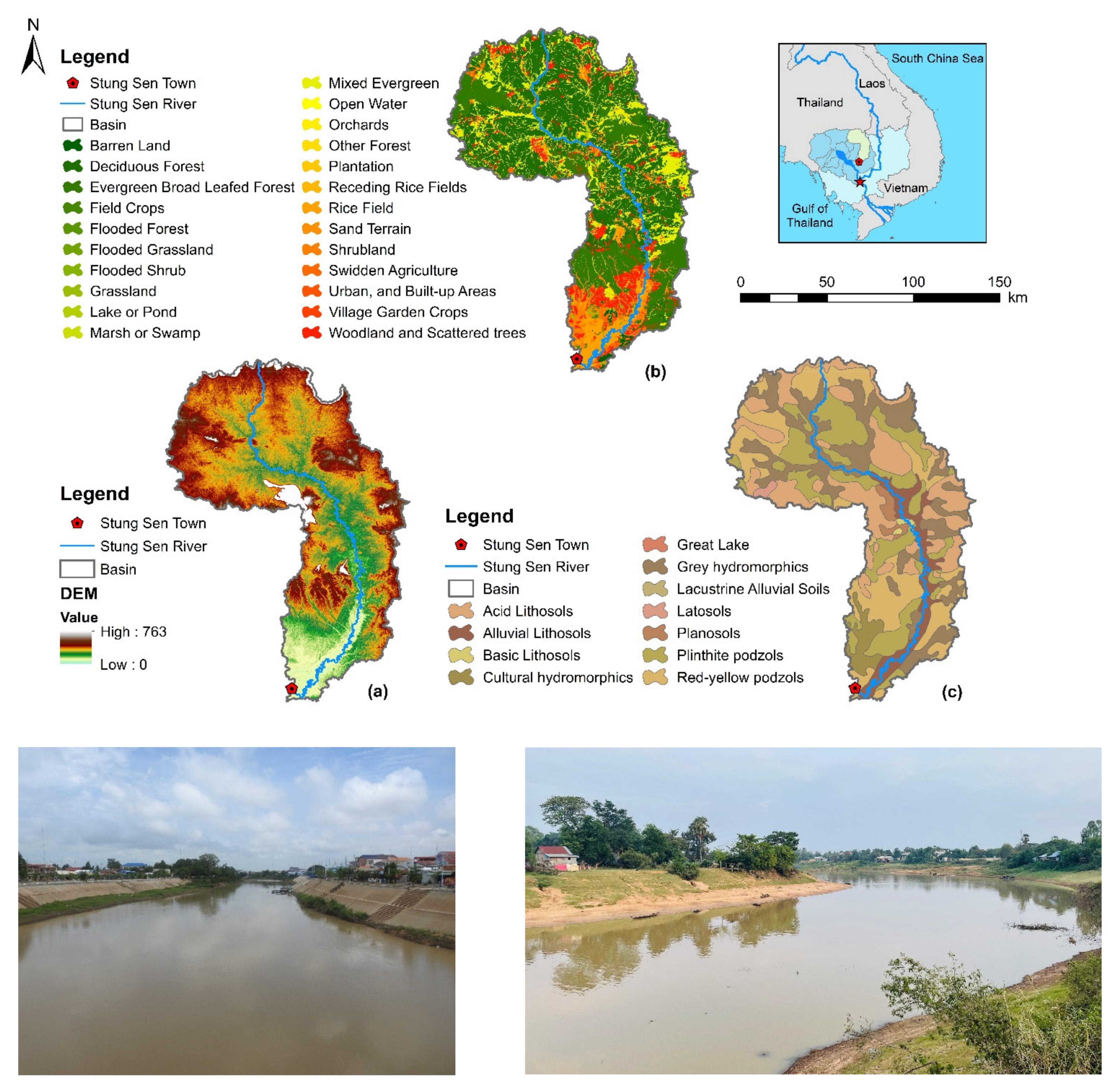
2.1. Sen River Basin, the Largest Sub-Basin of Tonle Sap Lake

Sen River Basin, the largest sub-basin of TSL, with a drainage area of about 16,000 km² (~20% of the TSL basin) and a length of 520 km (Figure 1). The catchment is medium hilly topography (with a maximum elevation of 750 m) in the upstream section but flat in the downstream section. The basin collects rainwater from the higher and middle reaches via tributary streams, which meander down an incised valley and into the lower reach, where the water enters the TSL and its floodplain. The basin is lowlands with moderate slopes and elevations of less than 100 m and is dominated by tropical monsoons.

2.2. Methods

2.2.1. SWAT Model Set-up

The Soil & Water Assessment Tool (SWAT), physically-based and semi-distributed, operates on a sub-daily to annual scale time step on a watershed scale. The SWAT model was developed to assess the impact of management on water, sediment, and agricultural chemical yields in ungauged catchments [40]. Catchments can be analyzed using the SWAT model by discretizing them into sub-basins and subdivided into HRUs (hydrological response units).

In this study, the SWAT model was set up to cover 14,140 km² of the Sen River Basin (~88% of the Sen River Basin). The precipitation used in this study was obtained from the Tropical Rainfall Measuring Mission (TRMM) [41] with ground observation bias correction using the linear scaling method [42,43,44]. The daily temperatures were obtained from SWAT global weather data. The study used topographic data from the Shuttle Radar Topography Mission (SRTM). Spatial data, including land use and soil type, were obtained from the Mekong River Commission (MRC) (

Table 1. Data input and sources in the SWAT model in this study.

Data Types	Description	Spatial Resolution	Temporal Resolution	Data Sources
Topography	Digital elevation model (DEM)	30 m		Shuttle Radar Topography Mission (SRTM) (http://srtm.csi.cgiar.org, accessed on 1 June 2021)
Land use/land-cover (LULC)	Land use classification	250 m × 250 m	2002	MoWRAM and MRC
Soil type	Soil types	250 m × 250 m	2002	MoWRAM and MRC
Precipitation	Observed rainfall TRMM	3 stations 18 stations	Daily, 1995–2019	DHRW of MOWRAM
Streamflow	Observed Streamflow	1 station	Daily, 2000–2019	DHRW of MOWRAM
Climate data	Gridded climate data	0.25°	Daily, 1997–2011	Global Weather Data for SWAT (globalweather.tamu.edu, accessed on 1 June 2021)
General Circulation Models (GCMs)	Climate Change Scenarios RCP2.6&8.5	Change factor in the subbasin	Monthly, 2030s and 2060s	MRC

). The study used static land use, while the dynamic change in land use could provide a differential effect; thus, the outcome only under conditions where current land use does not change drastically. However, the study serves to isolate the differential effects of climate change on water balance and flow regime.

In our model, this watershed had been discretized into small 51 sub-basins, and 1045 HRUs from 14 land uses, 20 soils, and five slope classes (0–2%, 2–5%, 5–15%, 15–25%, and >25%). The basin is covered mainly by deciduous (44.86%), followed by agricultural land-intensive evergreen, medium-low cover density (16.24%), mixed med-low cover density (13.43%), and many others (<10%). Sen River Basin is covered by Haplic Acrisol/Dystric Leptosol (20.6%), Ferric Acrisol (ACf/ACp) (16.84%), Ferric Acrisol (10.6%), Haplic Acrisol (10.23%), and many other soil types that are less than 10%.

The performance of the SWAT model was evaluated through the value of the Nash-Sutcliffe efficiency (NSE) [45], percentage bias (Pbias), and determination coefficient (R²). The NSE was used to determine how well the simulated result was against the observed data. If the NSE and R² for mean behaviors are greater than 0.60 and Pbias is within ±10, a calibrated model can be considered acceptable [46,47,48]. This study used the Rescaled Adjusted Partial Sums (RAPS) method to detect trends and fluctuations in the time series of observed and simulated flow:

$$RAP{S}_i={\displaystyle \sum _{n=1}^i\frac{T_n-T_m}{SD}}$$

where: T_n is the value of each sample in time series n = 1,2,3,…,i, and T_m is the mean value of the time series. SD represents the standard deviation [49].

2.2.2. Selected Climate Change Scenarios and GCMs

Climate change factors defined by the MRC to encompass the whole Mekong River were utilized as inputs to analyze the effects of climate change on the hydrological regime and water resources. The data was downscaled based on the climate change datasets of the IPCC 5th Assessment. The dataset provides monthly change factors for precipitation, temperature, solar radiation, and relative humidity [50]. Because it is a successful approach for generating data for climate change, the MRC used the change factor technique to estimate anticipated climate changes [32,51]. This study selected two scenarios, RCP2.6 and RCP8.5, with three different models in various time horizons. Based on the literature review, the suitable climate change models (GCMs) for the Lower Mekong are IPSL-CM5-MR, GISS-E2-R-CC, and GFDL-CM3 (

Table 2. The climate change scenarios and GCMs used in this study for future projection.

Emission Scenarios	Emission Rate	Time Horizon	GCMs Model
RCP 2.6	Low	Near future: 2030s (2021–2040) Medium Future: 2060s (2051–2070)	IPSL-CM5A-MR GISS-E2_CC GFDL-CM3
RCP 8.5	High	Near future: 2030s (2021–2040) Medium Future: 2060s (2051–2070)

).

2.2.3. Change in Flow Regime Evaluation

The Indicator of Hydrologic Alteration (IHA) was employed after the separating year using 33 hydrologic alteration parameters [52] to evaluate the different features of flow alteration under GCMs for RCP2.6 and RCP8.5. Hydrologic parameters in IHA Group 1: Magnitude of monthly water condition and IHA Group 2: Magnitude and duration of annual extreme condition were selected to illustrate the change in flow regimes (

Table 3. Hydrologic parameters used in the study.

General Group	Group 1: Magnitude of Monthly Water Condition	Group 2: Magnitude and Duration of Annual Extreme Condition
Regime features	Magnitude, Timing	Magnitude, Duration
Streamflow parameters	Mean value for each calendar month	Annual minimum 1-day means	Annual maximum 1-day means	Annual minimum 3-day means	Annual maximum 3-day means	Annual minimum 7-day means
		Annual maximum 7-day means	Annual minimum 30-day means	Annual maximum 30-day means	Annual minimum 90-day means	Annual maximum 90-day means

). These Group 1 and Group 2 parameters were used with historical and projected streamflow from the SWAT model and then compared across time horizons [53].

3. Results

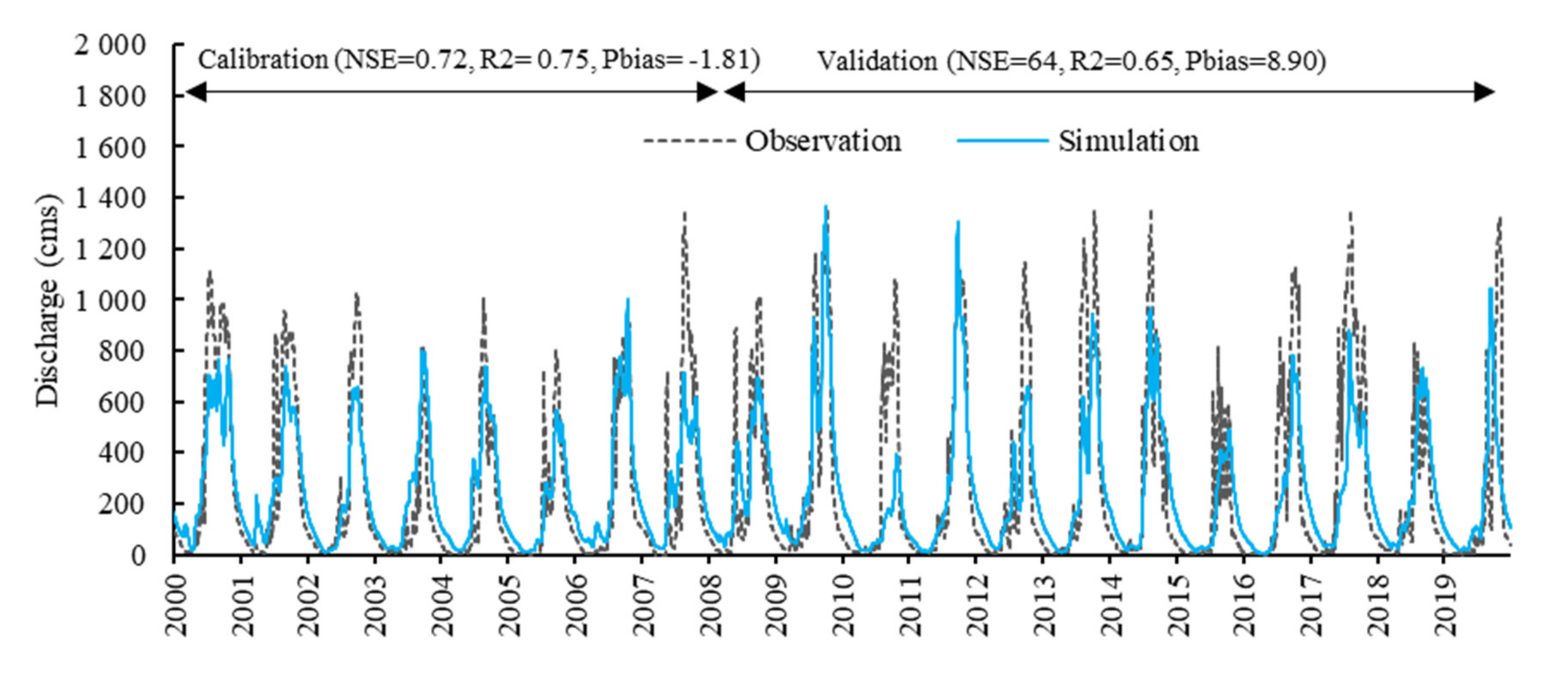
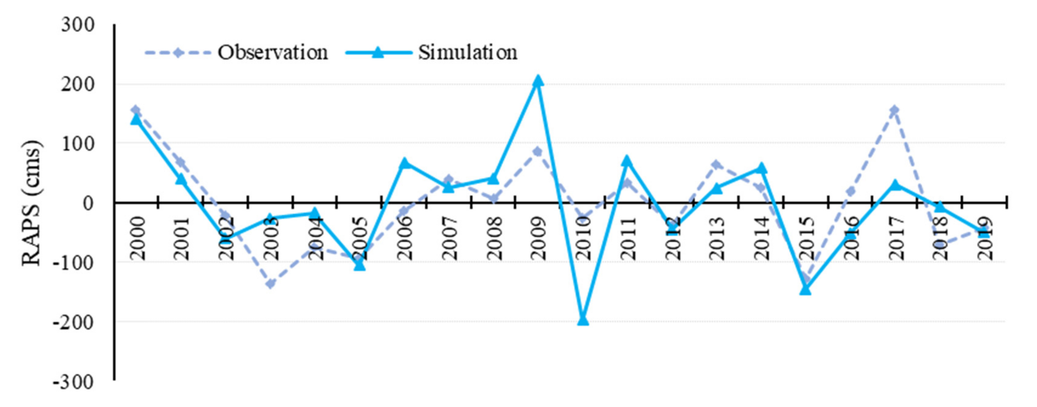
3.1. SWAT Model Performance

The mean annual rainfall was 1535 mm; 54% (827 mm) of the average annual rainfall was withdrawn by actual evapotranspiration, 36% (558 mm) became the streamflow, and another 10% for deep groundwater recharge from 2000 to 2019. The annual water yield of 558 mm comes from surface runoff (proportion of 43%), lateral flow (proportion of 25%), and groundwater (proportion of 32%). The calibration period covers 2000–2008 at daily step, while the validation period covers 2009–2019 (Figure 2). Based on the RAPS, both observed and simulated flow showed a similar trend and an agreement in a decrease in flow between 2000 and 2019. The statistical performance of the daily streamflow simulation suggested that the SWAT model was well-calibrated/validated and is in a satisfactory and good range in the Sen River Basin (

Table 4. Model performance for streamflow on a daily basis.

Period	Statistical Performance Measures
	NSE	Performance Evaluation	Pbias	Performance Evaluation	R2	Performance Evaluation
Calibration (2000–2008)	0.72	Good	−1.81	Very Good	0.75	Good
Validation (2009–2019)	0.64	Satisfactory	8.9	Good	0.65	Satisfactory

). Although the calibration and validation data are not separated, the graphical results show good performance for the calibration period and satisfactory performance for the validation period. The model produced the streamflow in an acceptable range at the start and end of the seasonal streamflow. However, certain peak-flow estimations were somewhat off. The overall model performance reasonably mirrored the observed flows for an independent dataset. The set-up SWAT model demonstrates enough potential to further process the procedure of climate change effect assessment within this range of daily streamflow performance.

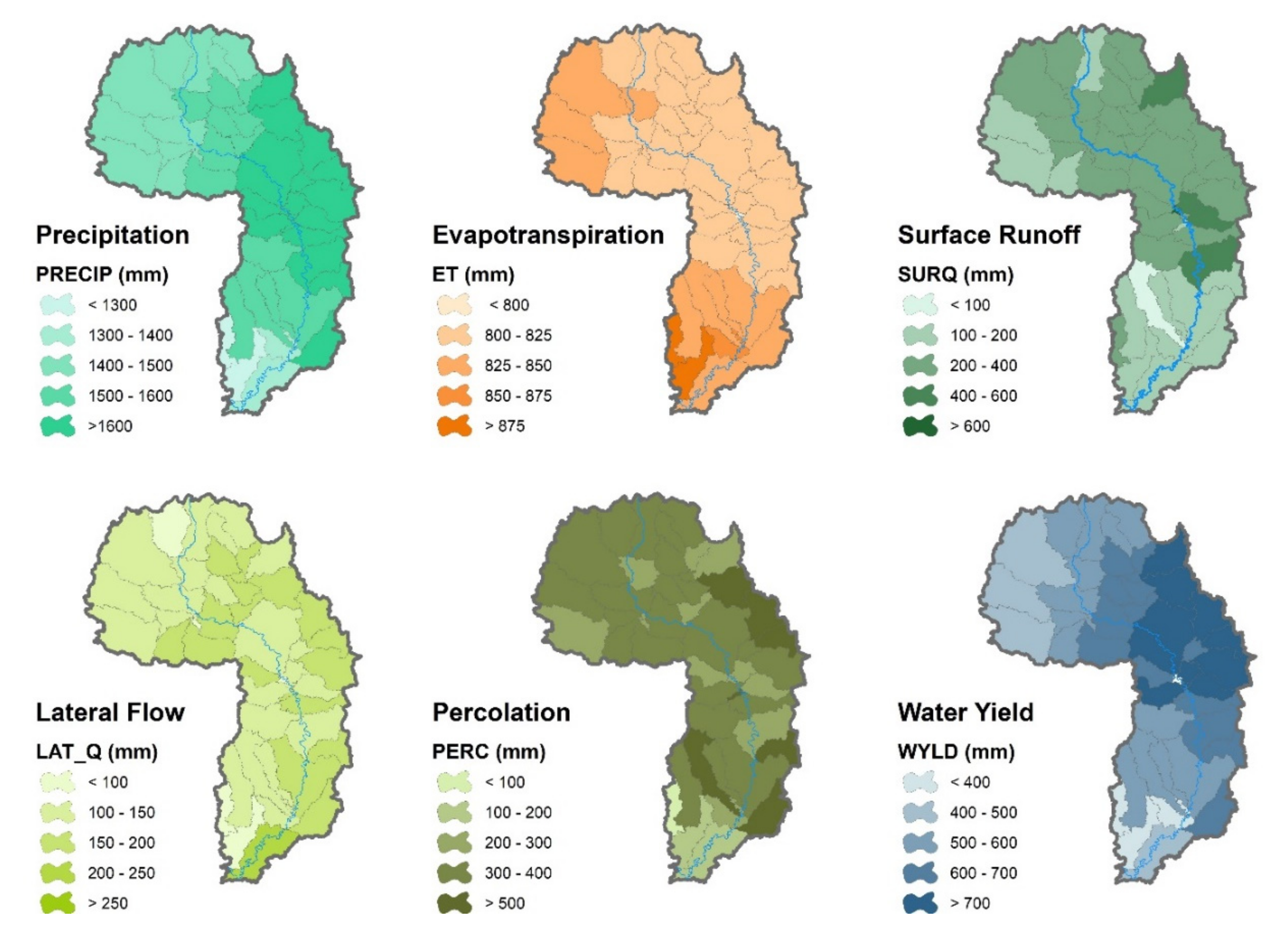
3.2. Assessment of Basin-Wide Water Balance

It was necessary to assess the baseline water balance and components to comprehend the detailed information in the Sen River Basin. It is ideal for analyzing and quantifying various hydrological components in the study area to address water management issues. In addition to the daily streamflow, the SWAT model calculated pertinent water balance components. Water balance components, including precipitation, evapotranspiration, lateral flow, surface runoff, and water yield of the baseline period from 2000 to 2019, were incorporated into the validated model output as hydrological components (Figure 3). This resulted in intra-annual hydrological component variation (

Table 5. Average monthly water balance components for the baseline period from 2000 to 2019.

Monthly	PRECIP	AET	SURQ	LATQ	GWQ	WYLD
		(mm/Month)
January	7.0	23.1	0.2	0.5	15	16.0
February	16.4	21.0	1.4	0.4	7	8.8
March	54.7	40.8	2.4	1.5	2	5.9
April	90.8	63.9	3.3	3.7	1	8.2
May	171.8	86.4	12.2	9.7	1	23.4
June	188.4	103.6	19.9	15.1	3	38.0
July	273.0	112.7	50.7	22.1	7	80.1
August	271.8	109.1	55.7	26.7	19	101.4
September	261.8	82.9	59.9	29.6	35	124.2
October	161.5	88.9	31.3	24.8	45	101.3
November	25.7	60.8	0.9	7.3	34	41.9
December	12.5	33.5	0.6	1.7	24	26.0

Note: PRECIP = precipitation, AET = actual evapotranspiration, SURQ = surface runoff contribution to streamflow, LATQ = lateral flow, GWQ = groundwater contribution to streamflow and WYLD = Water yield.

). The monthly contribution of water balance components is high in July, August, and October during the wet season and contributes low values from January to April. Actual evapotranspiration (AET) caused the most water loss from the basin among these components.

3.3. Climate Change Effect on Water Balance Components

3.3.1. Annual Change of Basin-Wide Water Balance Components

Table 6. Changes in basin-wide water balance terms (%) for near (2020–2040) and mid-century (2050–2070) relative to the baseline period (2000–2019) for each GCM.

Water Balance Term	Time	RCP 2.6			RCP 8.5
		GFDL	GISS	IPSL	GFDL	GISS	IPSL
		%
PRECIP	Near	2	−4	0	5	−11	−1
	Medium	1	−3	0	11	−23	−2
AET	Near	3	1	1	8	4	3
	Medium	2	1	1	18	5	5
Surface Runoff	Near	2	−10	−1	7	−29	−3
	Medium	2	−8	−1	16	−58	−4
Lateral flow	Near	1	−6	−1	2	−18	−3
	Medium	1	−5	−1	4	−36	−5
Groundwater flow	Near	−3	−19	−6	−8	−53	−18
	Medium	−2	−14	−5	−18	−96	−38
Water yield	Near	0	−12	−3	1	−34	−8
	Medium	0	−9	−2	2	−64	−15

shows the projected annual mean water balance components and their percentage change in the Sen River Basin for three different GCMs under two RCP scenarios for near and medium future periods at a basin scale. A higher average change percentage could be expected in almost every water balance component for the medium-term future (2060s) compared to the near-term future (2030s) under both RCP scenarios.

All water balance components (excepted AET and groundwater) were projected to increase during the 2030s and the 2060s for GFDL model under RCP2.6 and RCP8.5, while projected to decrease for the 2030s and the 2060s for GISS and IPSL model under RCP2.6 and RCP8.5 (Table 6). The AET was projected to increase for all models under both RCPs, while the highest annual AET was between 8% for the near-term future and 18% for the medium-term future. However, groundwater was projected to decrease for all GCMs under RCP2.6 and RCP8.5, while the greatest annual AET was between 8% for the near-term future and 18% for the medium-term future.

Annual rainfall could increase by 5 to 11% for the GCMs under the two RCP scenarios, respectively, for the near and medium-term. The greatest annual rainfall changes (11%) occur during the medium period, indicating that climate change in the basin is greater than in the mid-twentieth century under RCP8.5. The AET showed less change, with an increase of 1% and 1.2% (near-term future and medium-term future) for RCP2.6 and 2% and 4% (near-term future and medium-term future) for RCP8.5, respectively, while a decrease of 10% and 8% (near-term future and medium-term future) for RCP2.6 and 29% and 58% (near-term future and medium-term future) for RCP8.5.

3.3.2. Intra-Annual Change of Basin-Wide Water Balance Components

The projected mean monthly water balance components and their percentage of change compared to the baseline in different future GCMs are shown in

Table 7. Projected mean monthly water balance components and their percentage change in different future GCMs compared with the baseline under the RCP2.6 and RCP8.5 emission scenarios.

	RCPs		RCP 2.6						RCP 8.5
	Time Horizons	Baseline	Near			Mid			Near			Mid
	GCMs	(mm)	GFDL	GISS	IPSL	GFDL	GISS	IPSL	GFDL	GISS	IPSL	GFDL	GISS	IPSL
Rainfall	January	7	14	−4	−2	11	−3	−2	41	−11	−6	88	−24	−13
	February	16	1	−5	−8	0	−4	−6	2	−15	−22	3	−31	−47
	March	55	12	−13	−14	9	−10	−10	35	−38	−40	76	−82	−86
	Aprilil	91	−2	−3	−7	−2	−3	−6	−6	−10	−22	−13	−21	−47
	May	172	2	−6	−1	1	−4	−1	5	−17	−2	10	−37	−5
	June	188	1	−3	1	1	−2	1	3	−9	3	7	−19	7
	July	273	−1	−7	−3	−1	−5	−2	−4	−20	−8	−9	−42	−19
	August	272	1	−3	0	1	−2	0	4	−9	1	9	−19	3
	September	262	4	0	1	3	0	0	13	−1	2	27	−1	4
	October	161	2	−2	8	1	−1	6	5	−6	23	10	−13	49
	November	26	10	6	3	7	5	3	29	19	10	62	39	21
	December	12	5	−2	18	4	−1	14	15	−4	53	32	−10	113
Evapotranspiration	January	23	3	2	3	2	2	2	8	7	9	16	15	17
	February	21	3	−2	2	2	−1	1	9	−5	4	18	−12	5
	March	41	4	−3	−2	3	−2	−1	12	−9	−7	26	−29	−28
	April	64	6	−1	−1	4	−1	−1	17	−4	−6	38	−6	−11
	May	86	3	3	1	2	2	1	9	7	2	20	10	4
	June	104	2	1	1	2	1	1	7	1	4	14	−3	8
	July	113	4	3	2	3	2	2	11	7	6	24	9	14
	August	109	2	3	2	2	2	1	7	8	5	14	15	11
	September	83	1	2	0	1	2	0	4	7	1	9	14	2
	October	89	2	1	0	1	1	0	5	4	0	12	9	0
	November	61	2	1	2	1	1	2	5	3	7	10	6	15
	December	34	2	1	3	2	0	2	7	1	8	15	2	16
Water Yield	January	16	1	−12	0	1	−10	0	1	−38	−2	3	−86	−8
	February	9	−1	−13	−4	−1	−10	−3	−4	−39	−11	−5	−80	−22
	March	6	18	−24	−20	14	−18	−16	61	−57	−48	163	−83	−67
	April	8	0	−17	−22	0	−14	−18	2	−41	−51	5	−69	−76
	May	23	0	−20	−12	0	−16	−9	0	−50	−32	−2	−78	−56
	June	38	−1	−16	−5	0	−12	−4	−2	−42	−15	−5	−73	−31
	July	80	−5	−18	−8	−4	−14	−6	−13	−47	−23	−28	−82	−46
	August	101	−1	−13	−4	−1	−10	−3	−3	−36	−11	−6	−68	−23
	September	124	3	−7	−2	3	−6	−2	10	−23	−6	22	−41	−14
	October	101	1	−8	5	1	−6	4	3	−27	14	5	−56	30
	November	42	1	−10	0	1	−7	0	2	−31	0	4	−73	−3
	December	26	0	−11	1	0	−8	1	0	−34	2	0	−82	4

. Under the two scenarios and all timeframes, monthly rainfall in April and July was projected to increase, while monthly rainfall in November was projected to decrease (Table 7). Rainfall was projected to increase for the GFDL model from January to May, except for April, and decrease for the GISS and IPSL models in all time frames under the two climate scenarios; however, rainfall was expected to decline for the GISS model in June, August, September, October, and December, and to increase for IPSL and GFDL. The dry season rainfall was anticipated to lower consistently for GISS and IPSL models between the 2030s and 2060s in the two scenarios, but to increase between 1% and 14% for the GFDL model during the 2030s under all two scenarios.

The monthly evapotranspiration from May to January was expected to increase for all GCMs under both RCPs with all timeframes, while rainfall from February to April was projected to decrease for all GCMs (except GFDL) under both emission scenarios and in all time frames (Table 7). Evapotranspiration in rainy months was projected to increase from 1 to 24% for GCMs during 2030s and the 2060s. The evapotranspiration for the dry season was projected to steadily decrease for GISS and IPSL during the 2030s and 2060s under the two scenarios; however, it would increase between 2% and 38% for the GFDL model under all two scenarios during the 2030s.

Under both RCPs, the monthly water yield for all GCMs was projected to decrease in most months; however, the water yield for the GFDL model was projected to increase in January, March, April, May, September, and December. Under all scenarios, water yield in the dry season was projected to increase for the GFDL model in the 2030s and 2060s, while it was projected to decrease for the GISS and IPSL models. Water yield in the dry season was projected to increase for the GFDL model during 2030s and 2060s under all scenarios, while a decrease was predicted for the GISS and IPSL models. Rainfall during the rainy season was projected to consistently decrease for all GCMs for both RCPs.

The influence of precipitation changes features in changing monthly distributions of water budget components in the Sen River was investigated.

Table 8. Projected mean monthly water yield components and percentage changes in different GCMs compared to the baseline under RCP2.6 and RCP8.5.

	RCPs		RCP 2.6						RCP 8.5
	Time Horizons	Baseline	Near			Mid			Near			Mid
	GCMs	(mm)	GFDL	GISS	IPSL	GFDL	GISS	IPSL	GFDL	GISS	IPSL	GFDL	GISS	IPSL
Surface Runoff	January	0	58	11	11	47	11	0	84	−53	−11	321	−68	−58
	February	1	−7	−16	−20	−7	−15	−16	−21	−48	−49	−15	−71	−82
	March	2	42	−36	−37	32	−28	−29	140	−81	−84	380	−100	−100
	April	3	−7	−22	−33	−5	−18	−26	−18	−50	−71	−40	−78	−95
	May	12	1	−25	−14	1	−20	−11	3	−63	−38	2	−93	−68
	June	20	0	−17	−4	0	−13	−3	−1	−48	−14	−6	−84	−39
	July	51	−5	−18	−8	−4	−14	−6	−15	−51	−25	−32	−91	−53
	August	56	2	−9	0	1	−7	0	5	−28	−2	9	−68	−8
	September	60	8	−1	1	6	−1	1	25	−5	3	56	−18	5
	October	31	3	−5	16	2	−4	13	9	−14	52	19	−33	122
	November	1	27	16	11	20	11	8	91	47	34	234	103	75
	December	1	9	−10	48	7	−9	36	17	−33	143	55	−55	424
Lateral Flow	January	1	12	0	12	8	0	8	35	−2	33	75	−8	71
	February	0	8	−3	−3	8	−3	−3	26	−10	−13	59	−21	−23
	March	1	14	−14	−16	11	−10	−12	41	−41	−46	89	−76	−85
	April	4	5	−13	−17	4	−10	−13	14	−34	−46	28	−62	−79
	May	10	−1	−12	−8	−1	−9	−6	−2	−33	−23	−5	−60	−41
	June	15	0	−9	−2	0	−7	−2	0	−27	−7	0	−53	−11
	July	22	−2	−9	−3	−2	−7	−3	−7	−27	−9	−14	−56	−19
	August	27	−1	−7	−2	−1	−6	−2	−4	−22	−7	−8	−47	−13
	September	30	2	−3	0	2	−2	0	6	−9	0	13	−18	0
	October	25	2	−2	4	2	−2	3	6	−7	12	13	−14	24
	November	7	3	−2	6	2	−1	5	9	−4	18	19	−9	37
	December	2	5	−1	10	4	0	8	16	−1	30	35	−3	66
Groundwater	January	15	0	−13	−1	0	−10	−1	−1	−40	−3	−3	−89	−10
	February	7	−1	−13	−2	0	−10	−1	−2	−39	−4	−7	−85	−11
	March	2	−5	−17	−4	−4	−14	−3	−12	−42	−9	−28	−70	−19
	April	1	7	−17	−9	5	−14	−7	22	−38	−15	53	−64	−20
	May	1	−4	−30	−25	−3	−24	−20	−10	−54	−46	−18	−70	−49
	June	3	−4	−41	−28	−3	−33	−22	−14	−79	−63	−30	−92	−85
	July	7	−8	−40	−23	−6	−31	−18	−23	−84	−56	−45	−96	−84
	August	19	−9	−33	−17	−7	−25	−13	−25	−78	−46	−50	−100	−81
	September	35	−4	−22	−9	−3	−16	−7	−12	−65	−28	−30	−99	−61
	October	45	−1	−14	−3	−1	−11	−2	−4	−47	−10	−10	−94	−31
	November	34	0	−12	−1	0	−9	−1	−2	−39	−4	−5	−91	−14
	December	24	0	−12	−1	0	−9	−1	−1	−36	−3	−4	−89	−11

illustrates the monthly variations in water yield components in the Sen River Bain from GCMs for the 2030s and 2060s under two RCP scenarios. Under the two emission scenarios and all time frames, we found that monthly groundwater fell in all months for all GCMs. On the contrary, monthly surface runoff is expected to decrease in February, April, and July for all GCMs in the 2030s and 2060s under both emission scenarios, while the monthly lateral flow is projected to decrease in May, July, and August. The results indicated that monthly surface runoff and lateral flow might increase for the GFDL model and decrease for the GISS model, while the IPSL model may increase during the dry season and decrease during the rainy season. However, groundwater decreased during dry and wet seasons for all GCMs and both RCPs.

3.4. Climate Change on Flow Regimes

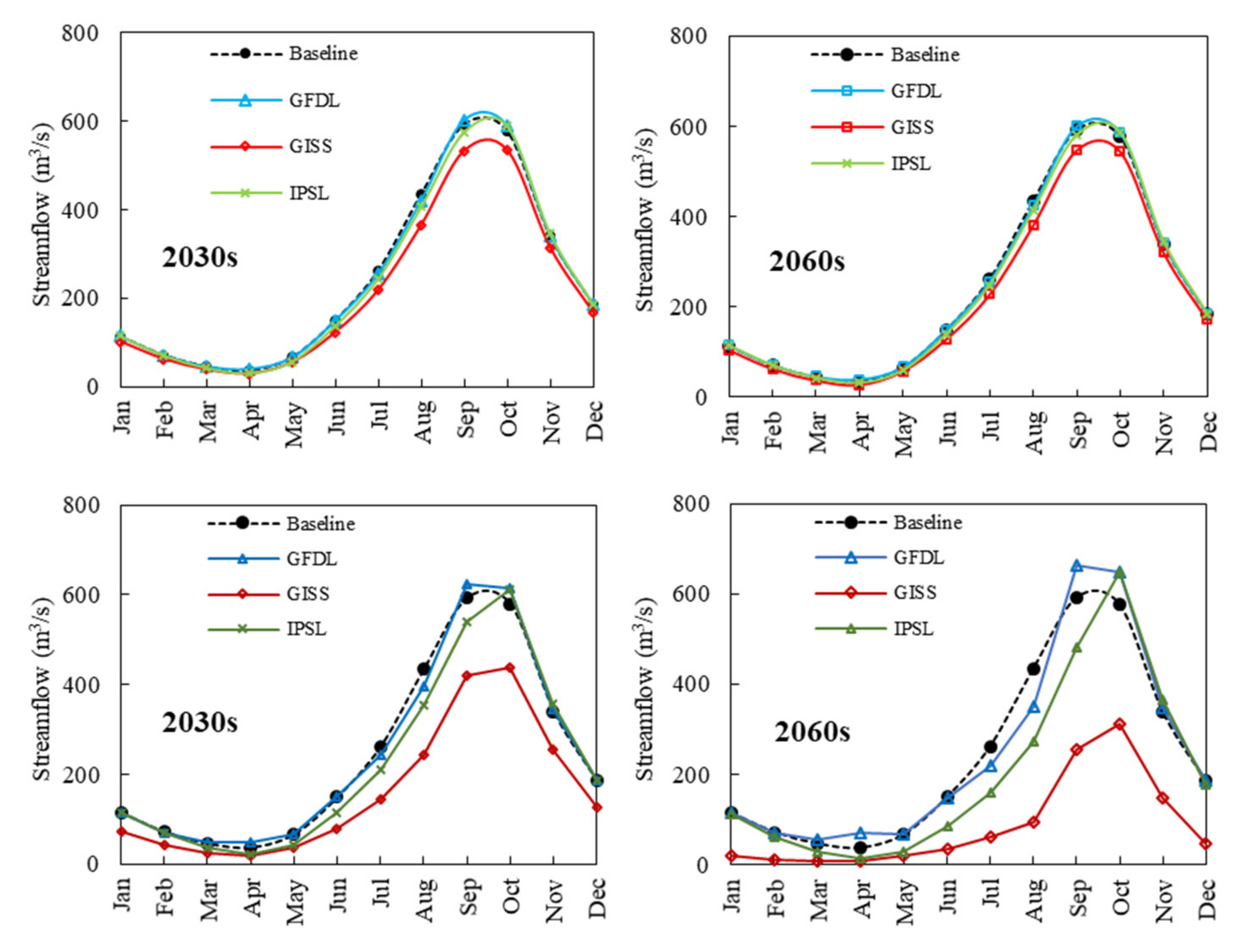
3.4.1. Changes in Intra-Annual Flow

The risk assessment of water resource development projects, such as hydropower, irrigation, and municipal water supplies, requires monthly variability under climate change. In addition, to respond to climate change, the construction of reservoir storage systems, which rely on monthly flow availability information, is needed. The change in monthly flow in RCP 2.6 is low throughout the year within the GFDL and IPSL models. The reduction in monthly flow can be noticed in the high flow season (June–October) under GISS model in both time horizons. While the change in the monthly projected flow in RCP8.5 is mostly negative, the peak seems to be high for GFDL and IPSL. Unsurprisingly, GISS show massive reductions every month of the year (Figure 4). The full range of changes in monthly flow is detailed in

Table 9. Percentage changes range in project mean monthly flows.

Month	PRC2.6						PRC8.5
	2030s			2060s			2030s			2060s
	GFDL	GISS	IPSL	GFDL	GISS	IPSL	GFDL	GISS	IPSL	GFDL	GISS	IPSL
May		↓↓	↓↓		↓↓	↓↓		↓↓↓	↓↓↓		↓↓↓↓	↓↓↓↓
June		↓↓	↓		↓↓	↓			↓↓			↓↓↓
July	↓	↓↓	↓	↓	↓↓	↓	↓		↓↓	↓↓		↓↓↓
August	↓	↓↓	↓	↓	↓↓	↓	↓		↓↓	↓↓		↓↓↓
September		↓	↓		↓	↓	↑		↓	↑↑		↓↓
October	↓	↓	↓		↓		↑		↑	↑↑		↑↑
November		↓			↓			↓↓↓	↑	↑	↓↓↓↓	↑
December		↓			↓							↓
January		↓↓			↓							↓
February		↓↓			↓↓				↓			↓↓
March		↓↓	↓		↓↓	↓	↑		↓↓	↑↑		↓↓↓
April	↑	↓↓	↓↓	↑	↓↓↓	↓↓	↑↑↑		↓↓↓	90		↓↓↓↓

Note: ↑/↓ = ±1–10%, ↑↑/↓↓ = ±10–20%, ↑↑↑ = +20–30%, ↓↓↓ = −(20–50)%, ↓↓↓↓ = −(50–85)%.

.

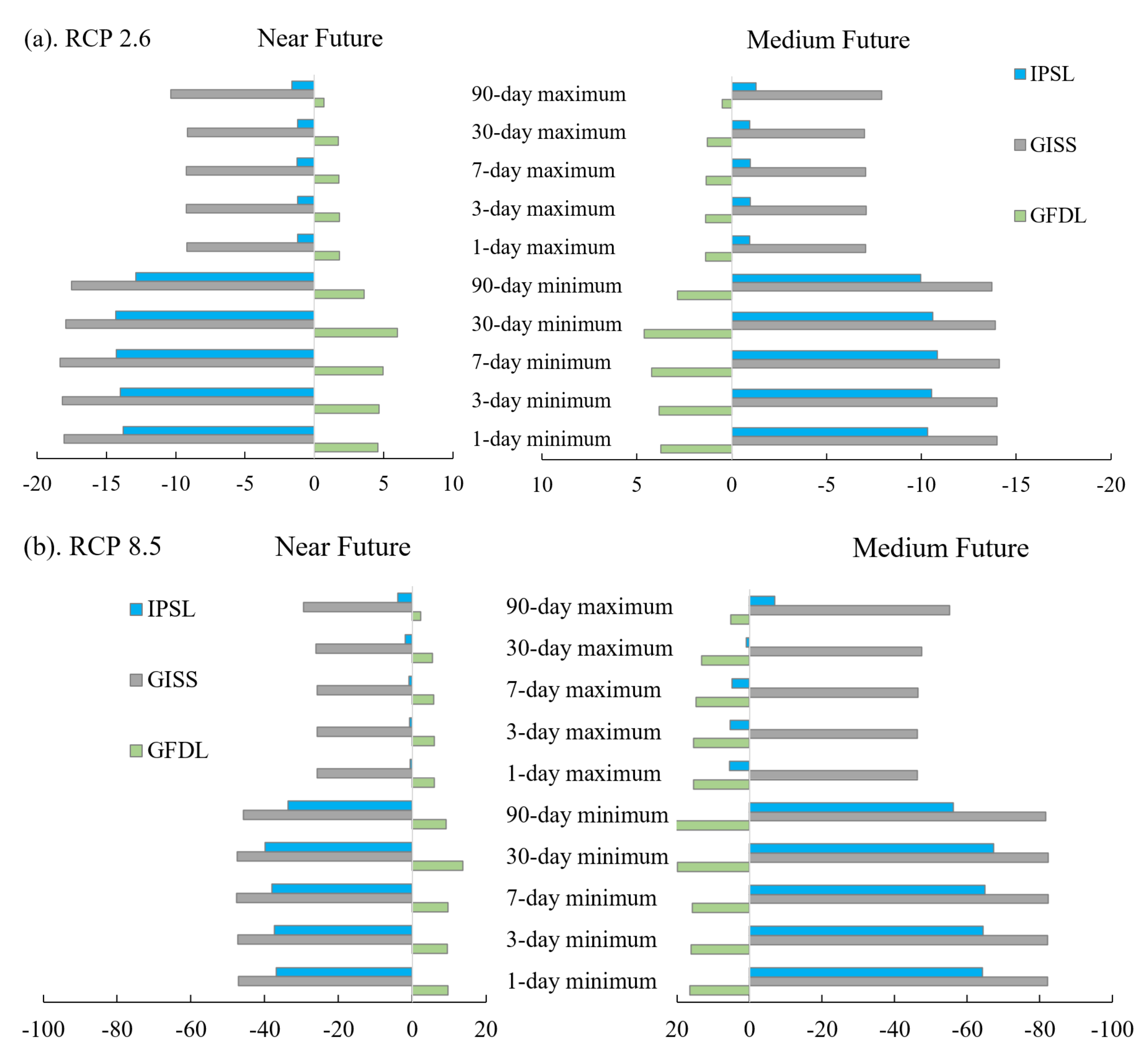
3.4.2. Changes in Extreme Flow

The high and low flow at the basin outlet were compared to capture the relative change of the three GCMs under RCP 2.6 and RCP 8.5 for the near future and medium future to the baseline period (

Table 10. Extreme flows and their percentage changes in the near future and medium future compared to the baseline period for the three GCMs under the RCP2.6 and RCP8.5 scenarios.

Flow Regimes	Baseline	Time Horizon	GFDL		GISS		IPSL
	(m3/s)		(m3/s)	(%)	(m3/s)	(%)	(m3/s)	(%)
RCP2.6
Q5	710.4	Near Future	719.0	1	641.6	−10	701.2	−1
		Medium Future	716.1	1	659.0	−7	705.3	−1
Q95	17.6	Near Future	17.9	2	15.0	−15	15.7	−11
		Medium Future	17.7	0	15.7	−11	16.2	−8
RCP8.5
Q5	710.4	Near Future	729.0	3	498.5	−30	676.7	−5
		Medium Future	754.0	6	329.8	−54	671.7	−5
Q95	17.6	Near Future	18.8	7	10.3	−42	12.0	−32
		Medium Future	19.6	11	3.1	−82	7.6	−57

). Under RCP 2.6, the high flow surpassing 5% of the time (Q₅) is expected to decline by 10% and 7% for GISS and about 1.2% and 1% for IPSL in the near and medium future, respectively, and under RCP 8.5, the high flow is expected to rise by 30% in the near future and decline by 54% in the medium future for GISS, while declining by 5% in both the near future and medium future for IPSL. Low flow exceeding 95% of the time (Q₉₅) and fluctuations in flow values justify the demand for storage construction within the focus area.

For the Q₅, in the 2030s, two GCMs (GISS and IPSL) suggested a decrease of 10 to 30% and 1 to 5%, whereas GFDL predicted an increase of 1% to 3% for RCP2.6 and RCP8.5, respectively. Moreover, the Q₅ is likely to decrease by 7−54% for GISS and 1−5% for IPSL, but GFDL will increase by 1% and 6% for RCP2.6 and RCP8.5 in the 2060s, respectively. These results demonstrated that future flood magnitudes in the Sen River Basin would rise slightly for the GFDL model while reducing for the GISS and IPSL models in the 2030s and 2060s.

For the Q₉₅ in the 2030s, streamflow is predicted to increase by 2% and 7% by the GFDL model and, in the same period, to decrease from 15−42% and 11−32% by the other two models for RCP2.6 and RCP8.5, respectively. In the 2060s, Q₉₅ is expected to increase and decrease in a higher magnitude than in the 2030s. It would increase by 0−11% for the GFDL model, but it would decrease from 11−82% and 8−57% through the GISS and IPSL models for RCP2.6 and RCP8.5, respectively. The significant decrease in Q₉₅ projected by the GISS model indicated that the drought event would significantly increase in 2030s and 2060s.

The flow duration curve was also evaluated by comparing the baseline and expected streamflow (Figure 5). This assessment aimed to test the absolute value of the streamflow for information to evaluate flow regimes as part of environmental flow prediction in ungauged watersheds or scenario analysis. Due to the low change in monthly flow, RCP2.6 produced a low change in flow duration. With this association with the monthly flow, RCP8.6 caused more alternated flow, particularly GISS and high flow.

3.4.3. Changes in Multiple Temporal Scales of Flow under Different Climate Scenarios

Design floods are typically estimated using maximum instantaneous flows [54,55]. Annual one-day maximum floods and instantaneous floods are positively associated [56]. As a result, the impact of CC on instantaneous flows is considered the same as the annual one-day maximum flow. This section focused on the minimums and maximums of streamflow on 1-day, 3-day, 7-day, 30-day, and 90-day. It is clear that all simulated flows reach the maximum and the minimum in the 1-day condition, and the highest percentage change is likely in the 90-day minimum condition, while the lowest percentage of flow change is in the 1-day maximum condition (Figure 6).

The negative trends under RC2.6 are significant, decreasing at least 10% for GISS and IPSL, increasing the GFDL model by less than 6% for the 1-day, 3-day, 7-day, 30-day, and 90-day annual minimum flows for both time horizons. For the 1-day, 3-day, 7-day, 30-day, and 90-day annual maximum flows, the GFDL under RCP2.6 increases slightly, less than 2% for the 2030s and 2060s, whereas IPSL reveals a reduction. Unlike the GFDL and IPSL, the GISS model demonstrates that the negative trends under both scenarios are remarkable. Under RCP8.5, the variations are partially remarkable, especially for the 2060s, decreasing more than 50% in the GISS and IPSL models for the 1-day, 3-day, 7-day, 30-day, and 90-day annual minimum flows. In comparison, the GFDL reveals positive trends for the same time horizon. For the 2030s time horizon, the GISS and IPSL models show negative trends, whereas GFDL increases by a small proportion.

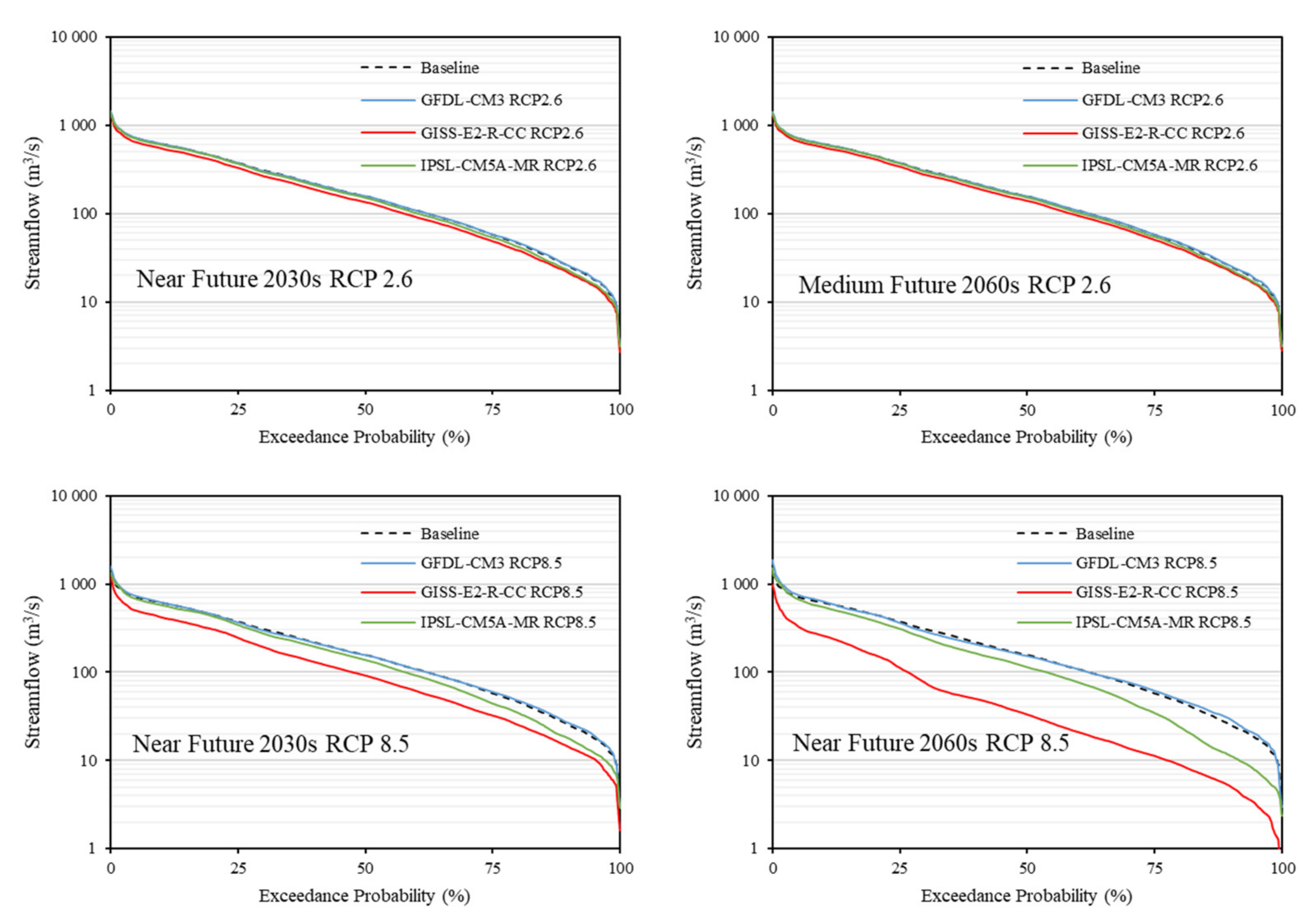
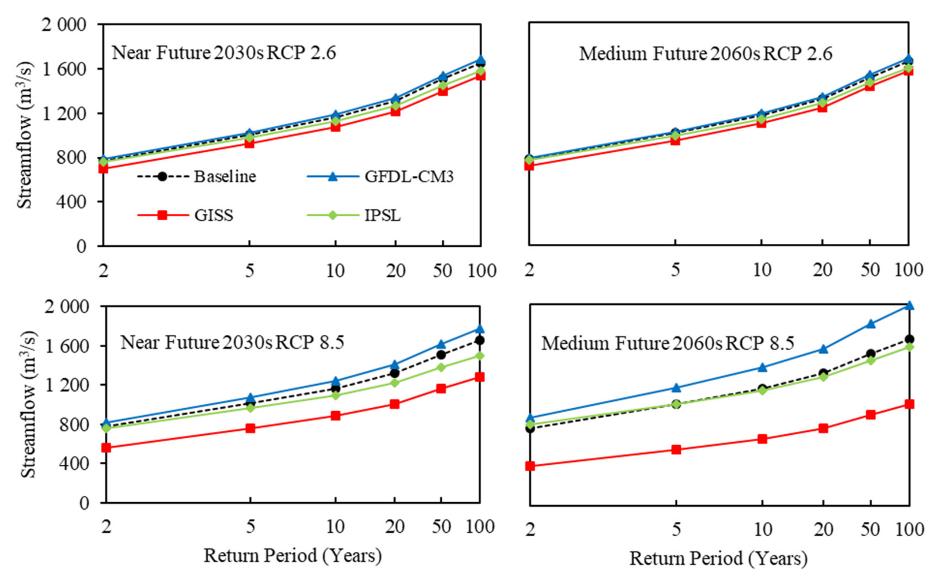
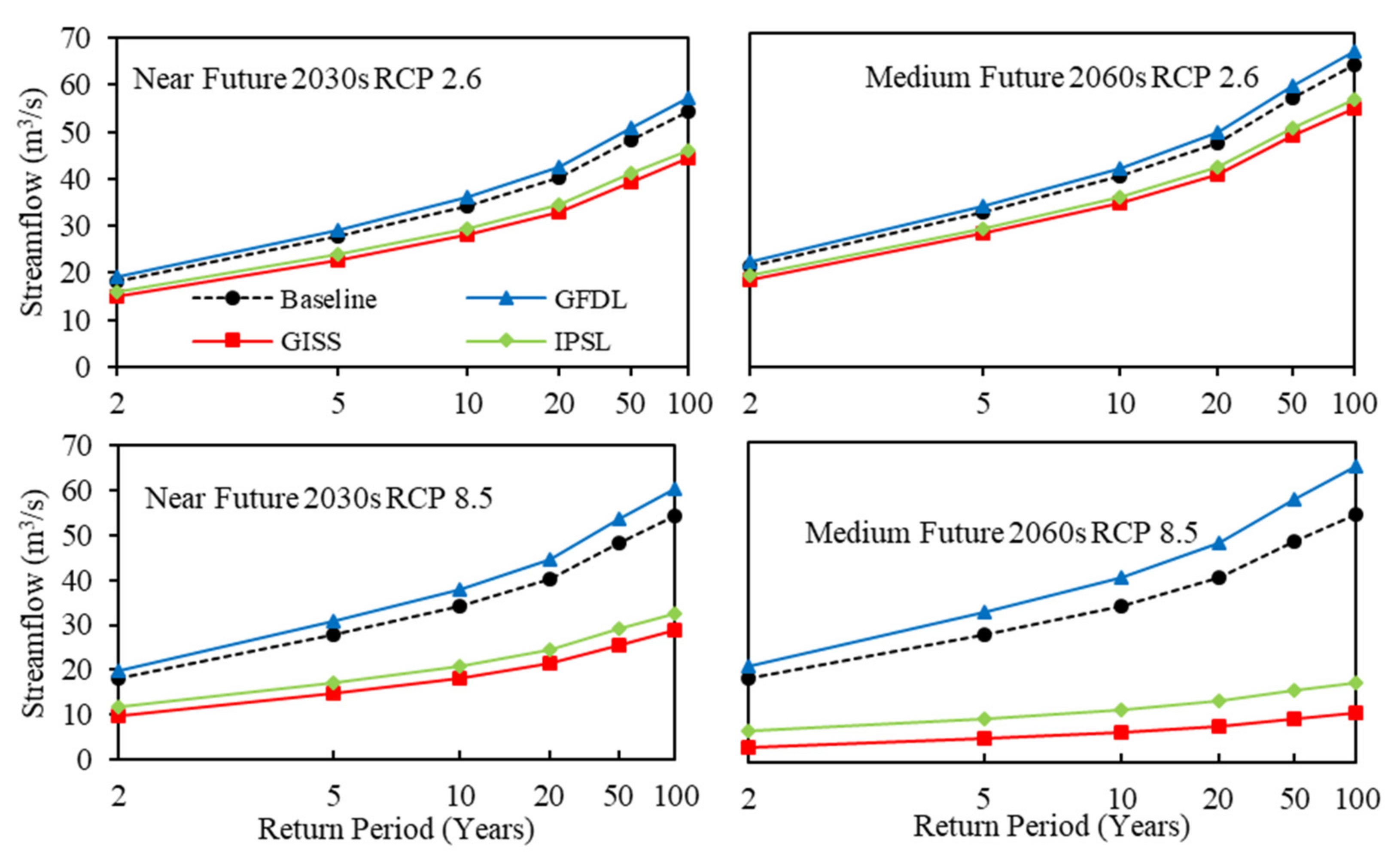
3.4.4. Change in Frequency Analysis of Flow

The frequency analysis of this study focused on annual one-day maximum and annual one-day minimum flows carried out by the Gumbel distribution and the maximum likelihood method. Changes in the one-day maximum flow and one-day minimum flow for the different GCMs and return periods are given in Figure 7 and Figure 8, including baseline values. The baseline floods for the 5-, 10-, and 50-year return periods were 1010, 1166, and 1509 m³/s. Figure 7 reveals that the one-day maximum flood resulting from baseline is higher than the GISS and IPSL models flood for both scenarios and time horizons for the considered return periods, whereas the GFDL model shows greater magnitude than baseline. It can be observed that flood magnitudes vary in RCP8.5 compared to RCP2.6.

The range of change in one-day minimum flow due to climate change regarding the baseline condition is between −18% (near future/50 /100 years) and 5% (near future/100 years) for RCP2.6, while it is between −8% (medium future/2 years) and 2% (medium future/100 years) for the RCP 8.5 scenario (Figure 8). Almost half of the flow values in RCP 2.6 are expected to decrease by more than 10%. This phenomenon is mainly observed in the near future and in the medium future. Similar results were obtained in RCP 8.5, i.e., nearly 6% of the low flows declined concerning the base case values.

4. Discussion

The possible implications of climate change on the hydrological process and river flow in the Sen River Basin were assessed through modeling work. The future climate of the basin was projected using three general circulation models (GFDL-CM3, GISS-E2-R-CC, and IPSL-CM5A-MR) for low-emission scenarios (RCP2.6) and high-emission scenarios (RCP8.5). In addition, the assessment of the potential implications of climate change on river flow considered two time horizons: the near-term period (2030s) and the medium-term period (2060s).

4.1. Correlation between the Variation of Precipitation and Water Budget

A correlation analysis was conducted on the projected monthly precipitation change and monthly water budget components (

Table 11. Correlation coefficients for the relationship between monthly projected precipitation change and monthly projected water budget component change.

	RAIN	SURF_Q	LAT_Q	GW_Q	WYLD	ET	PET
RAIN	1	0.96	0.78	0.40	0.78	0.36	−0.40	RCP8.5
SURF_Q	0.89	1	0.79	0.44	0.82	0.36	−0.46
LAT_Q	0.77	0.84	1	0.65	0.85	0.50	−0.34
GW_Q	0.51	0.52	0.75	1	0.74	0.18	−0.16
WYLD	0.85	0.83	0.88	0.73	1	0.41	−0.33
ET	0.27	0.36	0.48	0.27	0.42	1	0.430
PET	−0.52	−0.45	−0.41	−0.18	−0.42	0.36	1
	RCP2.6

). Surface runoff and predicted precipitation have a strong positive correlation with both RCP2.6 and RCP8.5. From this basin-wide perspective, variations in precipitation will have the most significant influence on surface runoff, resulting in a change in water yield as a streamflow. The high correlation between anticipated precipitation and projected water yield change is the cause of changing streamflow, which results in an extreme change in high flow (Q₅) and low flow (Q₉₅), as indicated in Section 3.4.2. At the same time, the sub-basin may experience a flash flood because of the high connection between future precipitation and future surface runoff alterations.

4.2. Change in Water Balance and Flow Regime across the Timescale, RCPs, GCMs, and Regional Scale

The prediction results depend on the climate model used. GISS model yielded 1%; −19% and 5%; −96% changes in water balances for RCP2.6 and RCP8.5, respectively, while the GFDL and IPSL models remained around 3%; −3% for RCP2.6 and 18%; −18% for RCP8.5 and 1%; −6% for RCP2.6 and 5%; −38% for RCP8.5, respectively (Table 6). The RCPs ranged from very high (RCP8.5) to very low (RCP2.6) future concentrations. RCP 8.5 leads to much greater temperature increases, which means greater impacts and greater costs. Previous studies in the Mekong Region [57,58] noted that the projections of river flow change are highly dependent upon the GCM used regarding the direction and magnitude of projected changes in precipitation produced by different GCMs. Due to the pattern of change for the GISS model, which is the drier pattern for precipitation, the water balance tends to change negatively for both scenarios. Similarly, the study of climate simulation with the GISS model by [59] found that the precipitation and surface runoff were likely to decrease due to the effect of direct and indirect aerosol. It can be argued that the GISS model will follow the negative trend for water balance. However, owing to the high surface temperature change GISS model compared to the GFDL and IPSL models [60], the GISS model showed more significant changes in water balance than the GFDL and IPSL models. These results are parallel with the study of [34], which found that the streamflow for the GISS model negatively changes greater than GFDL and IPSL for three different time horizons (2030s, 2060s, and 2090s) in the Sen River Basin. The annual mean precipitation changes range from −11% to 5% for the near future across the GCMs and even −23% to 11% for the medium future. The relative fluctuations in monthly precipitation, on the other hand, are considerable. Due to the low amount of rainfall, the highest change in future monthly precipitation is expected to take place in the dry season. The smaller range of change in the rainy season. Rainfall is expected to decrease in both the dry and rainy seasons for GISS and IPSL in both time horizons and RCPs. Under the GFDL model, the rainfall expects to increase in both time horizons and RCPs. It can be highlighted that owing to GCMs, emission scenarios, and different timescales, the uncertainty in projected precipitation, PET, and streamflow projections is extensive. From the perspective of monthly and annual streamflow change, the impact of climate change on changes in monthly streamflow is more significant than annual streamflow. A considerable reduction of between 10–20% in monthly runoff could be found in the rainy season under RCP2.6. Under RCP8.5, the decrease in monthly flow can be between 20–50% for GISS and IPSL models. When considering the change in the precipitation and streamflow, it is concluded that even minor variations in precipitation may have a considerable impact on streamflow. The decrease in precipitation and streamflow in both dry and rainy seasons will cause drought in the basin. The result also aligns with [34] that it will be more likely that the Tonle Sap area will experience extreme droughts rather than floods, which will impact future freshwater availability by reducing both the annual and seasonal flow. Climate change in the Lower Mekong region [61,62] will experience drier and longer dry seasons and lower precipitation in future climate projections.

4.3. The Perspectives for Further Investigation

In this study, climate change was considered the primary cause of streamflow changes. However, other factors, such as land-use change, could affect the hydrological process in Sen River Basin. This study used static land use, which could have affected the performance of the model. The change in forest cover could be distributed to cut off the differential effect of climate change on runoff [34]. One important driver worth mentioning is that the effects of water infrastructure development projects, such as irrigation schemes and water allocation, could significantly impact water availability in the near future compared to the direct effects of climate change [34]. Such conclusions about climate change impact are conditional and dependent upon future GCMs and approaches used in this study. One such limitation is that the data acquired from TRMM with bias correction with observed rainfall and the number of variables accessible to weather for the analysis was somewhat limited. A more comprehensive downscaling method is recommended, as different downscaling methods might result in varied future climate estimates [63]. The streamflow simulation can be more affected by the selection of downscaling methods [64,65,66]. However, it is still a question of which technique performs better than the others [67]. The study attempted to assess the uncertainty in the projected hydrological process and streamflow associated with three GCMs under two emission scenarios. However, many more different GCMs could cause variations in annual streamflow, showing that the CMIP5 GCMs may consist of many uncertainties [58,68]. Because of the simplicity and low computation cost of the change factor downscaling approach, it is beneficial to apply multiple GCMs in long-term hydro-climatic assessment [69]. However, the local topography and micro-climatic system, which could produce less accuracy in predicting short-term extreme precipitation events, were not considered in this approach; thus, it could cause some uncertainties in hydro-climatic studies [70]. Therefore, the impacts of different downscaling approaches should be further explored.

5. Conclusions

This study determined the possible effects of future climate scenarios on the hydrological process and hydrological extremes in the Sen River Basin. The set-up SWAT Model for analyzing the effect of future climate change in the Sen River Basin was considered to have the capacity to represent the watershed properly. The hydrological response of the basin was simulated using the daily streamflow under three GCMs (GFDL-CM3, GISS-E2-R-CC, and IPSL-CM5A-MR) for the future climate projection RCP2.6 and RCP8.5 emission scenarios. In comparison to the baseline, IHA was used to analyze the influence of climate change on flow variation. The daily flow records (2000–2019) from the Kampong station within the Sen River Basin were chosen to evaluate the influence of climate change on hydrologic regime alteration. Two-time series (baseline period and future under climate change) flow were taken into consideration. The principal conclusions are as follows:

• Between 2000 and 2019, the annual distribution pattern of streamflow changed. Climate change profoundly affecting the flow regime would be positively altered (an increase compared to baseline) with the GFDL-CM3 model under both RCPs in all future periods; at the same time, GISS-E2-R-CC and IPSL-CM5A-MR models would be negatively altered (decrease compared to baseline) in the Sen River Basin. Generally, the annual peak and the range of monthly discharges declined, while the number of reversals in discharge expanded. Moreover, they altered the timing of high and low flows and varied the timing of the annual maximum and minimum flows.
• Compared to the baseline period, hydrologic characteristics illustrated significant changes in the future under climate change. The magnitude of flow (GISS-E2-R-CC and IPSL-CM5A-MR models) was lesser compared to baseline, and the frequency of low flow events decreased throughout the year; the maximum flows and minimum flows (from 1-, 3-, 7-, 30-, and 90-day) were reduced. Another model (GFDL-CM3) discussed the different tendencies, so the prediction results depend on the model used.
• Indicators of hydrologic alteration in accordance with the components of the hydrologic regime can be utilized to measure the level of change induced by climate change and are further related to ecological responses of the fluvial ecosystem.

In this study, we suggest developing flexible strategies for water management in the Sen River Basin for the most efficient use of the available water, which is highly variable.

References

1. Tamm, O.; Maasikamäe, S.; Padari, A.; Tamm, T. Modelling the effects of land use and climate change on the water resources in the eastern Baltic Sea region using the SWAT model. Catena 2018, 167, 78–89. [Google Scholar] [CrossRef]
2. Kodra, E.; Ghosh, S.; Ganguly, A.R. Evaluation of global climate models for Indian monsoon climatology. Environ. Res. Lett. 2012, 7, 014012. [Google Scholar] [CrossRef]
3. Johnston, R.; Smakhtin, V. Hydrological modeling of large river basins: How much is enough? Water Resour. Manag. 2014, 28, 2695–2730. [Google Scholar] [CrossRef] [Green Version]
4. Delgado, J.M.; Apel, H.; Merz, B. Flood trends and variability in the Mekong river. Hydrol. Earth Syst. Sci. Discuss. 2009, 14, 407–418. [Google Scholar] [CrossRef] [Green Version]
5. Holman, I.P. Climate change impacts on groundwater recharge-uncertainty, shortcomings, and the way forward? Hydrogeol. J. 2006, 14, 637–647. [Google Scholar] [CrossRef] [Green Version]
6. Zhu, J. Impact of climate change on extreme rainfall across the United States. J. Hydrol. Eng. 2013, 18, 1301–1309. [Google Scholar] [CrossRef]
7. Muhammad, M.K.I.; Nashwan, M.S.; Shahid, S.; Ismail, T.B.; Song, Y.H.; Chung, E.-S. Evaluation of empirical reference evapotranspiration models using compromise programming: A case study of Peninsular Malaysia. Sustainability 2019, 11, 4267. [Google Scholar] [CrossRef] [Green Version]
8. Kadkhodazadeh, M.; Anaraki, M.V.; Morshed-Bozorgdel, A.; Farzin, S. A new methodology for reference evapotranspiration prediction and uncertainty analysis under climate change conditions based on machine learning, multi criteria decision making and Monte Carlo methods. Sustainability 2022, 14, 2601. [Google Scholar] [CrossRef]
9. Trisurat, Y.; Aekakkararungroj, A.; Ma, H.-O.; Johnston, J.M. Basin-wide impacts of climate change on ecosystem services in the Lower Mekong Basin. Ecol. Res. 2018, 33, 73–86. [Google Scholar] [CrossRef]
10. Arnell, N.W. Climate change and global water resources. Glob. Environ. Chang. 1999, 9, S31–S49. [Google Scholar] [CrossRef]
11. Bolch, T.; Kulkarni, A.; Kääb, A.; Huggel, C.; Paul, F.; Cogley, J.G.; Frey, H.; Kargel, J.S.; Fujita, K.; Scheel, M. The state and fate of Himalayan glaciers. Science 2012, 336, 310–314. [Google Scholar] [CrossRef] [PubMed] [Green Version]
12. Wang, G.; Zhang, J.; Xuan, Y.; Liu, J.; Jin, J.; Bao, Z.; He, R.; Liu, C.; Liu, Y.; Yan, X. Simulating the impact of climate change on runoff in a typical river catchment of the Loess Plateau, China. J. Hydrometeorol. 2013, 14, 1553–1561. [Google Scholar] [CrossRef]
13. Intergovernmental Panel On Climate Change. Climat Change; Intergovernmental Panel On Climate Change: Geneva, Switzerland, 2014. [Google Scholar]
14. Pierce, D.W.; Barnett, T.P.; Santer, B.D.; Gleckler, P.J. Selecting global climate models for regional climate change studies. Proc. Natl. Acad. Sci. USA 2009, 106, 8441–8446. [Google Scholar] [CrossRef] [PubMed] [Green Version]
15. Arnell, N.W. Effects of IPCC SRES* emissions scenarios on river runoff: A global perspective. Hydrol. Earth Syst. Sci. 2003, 7, 619–641. [Google Scholar] [CrossRef] [Green Version]
16. Arnell, N.W.; Gosling, S.N. The impacts of climate change on river flow regimes at the global scale. J. Hydrol. 2013, 486, 351–364. [Google Scholar] [CrossRef]
17. Nohara, D.; Kitoh, A.; Hosaka, M.; Oki, T. Impact of climate change on river discharge projected by multimodel ensemble. J. Hydrometeorol. 2006, 7, 1076–1089. [Google Scholar] [CrossRef] [Green Version]
18. Gosling, S.; Taylor, R.G.; Arnell, N.; Todd, M. A comparative analysis of projected impacts of climate change on river runoff from global and catchment-scale hydrological models. Hydrol. Earth Syst. Sci. 2011, 15, 279–294. [Google Scholar] [CrossRef] [Green Version]
19. Gosling, S.N.; Bretherton, D.; Haines, K.; Arnell, N.W. Global hydrology modelling and uncertainty: Running multiple ensembles with a campus grid. Philos. Trans. R. Soc. A Math. Phys. Eng. Sci. 2010, 368, 4005–4021. [Google Scholar] [CrossRef]
20. Andréasson, J.; Bergström, S.; Carlsson, B.; Graham, L.P.; Lindström, G. Hydrological change–climate change impact simulations for Sweden. AMBIO J. Hum. Environ. 2004, 33, 228–234. [Google Scholar] [CrossRef]
21. Conway, D. The impacts of climate variability and future climate change in the Nile Basin on water resources in Egypt. Int. J. Water Resour. Dev. 1996, 12, 277–296. [Google Scholar] [CrossRef]
22. Nijssen, B.; O’Donnell, G.M.; Hamlet, A.F.; Lettenmaier, D.P. Hydrologic sensitivity of global rivers to climate change. Clim. Chang. 2001, 50, 143–175. [Google Scholar] [CrossRef]
23. Thompson, J. Modelling the impacts of climate change on upland catchments in southwest Scotland using MIKE SHE and the UKCP09 probabilistic projections. Hydrol. Res. 2012, 43, 507–530. [Google Scholar] [CrossRef]
24. Thompson, J.; Gavin, H.; Refsgaard, A.; Sørenson, H.R.; Gowing, D. Modelling the hydrological impacts of climate change on UK lowland wet grassland. Wetl. Ecol. Manag. 2009, 17, 503–523. [Google Scholar] [CrossRef] [Green Version]
25. Chun, K.; Wheater, H.; Onof, C. Streamflow estimation for six UK catchments under future climate scenarios. Hydrol. Res. 2009, 40, 96–112. [Google Scholar] [CrossRef]
26. Gosling, S.N. The likelihood and potential impact of future change in the large-scale climate-earth system on ecosystem services. Environ. Sci. Policy 2013, 27, S15–S31. [Google Scholar] [CrossRef]
27. Thompson, J.; Green, A.; Kingston, D. Potential evapotranspiration-related uncertainty in climate change impacts on river flow: An assessment for the Mekong River basin. J. Hydrol. 2014, 510, 259–279. [Google Scholar] [CrossRef] [Green Version]
28. Bhatta, B.; Shrestha, S.; Shrestha, P.K.; Talchabhadel, R. Evaluation and application of a SWAT model to assess the climate change impact on the hydrology of the Himalayan River Basin. Catena 2019, 181, 104082. [Google Scholar] [CrossRef]
29. Taylor, K.E.; Stouffer, R.J.; Meehl, G.A. An overview of CMIP5 and the experiment design. Bull. Am. Meteorol. Soc. 2012, 93, 485–498. [Google Scholar] [CrossRef] [Green Version]
30. Yang, J.; Yang, Y.E.; Chang, J.; Zhang, J.; Yao, J. Impact of dam development and climate change on hydroecological conditions and natural hazard risk in the Mekong River Basin. J. Hydrol. 2019, 579, 124177. [Google Scholar] [CrossRef]
31. Shrestha, S.; Bhatta, B.; Shrestha, M.; Shrestha, P.K. Integrated assessment of the climate and landuse change impact on hydrology and water quality in the Songkhram River Basin, Thailand. Sci. Total Environ. 2018, 643, 1610–1622. [Google Scholar] [CrossRef]
32. Mekong River Commission (MRC). Summary of the Basin-Wide Assessments of Climate Change Impacts on Water and Waterrelated Resources in the Lower Mekong Basin; MRC: Vientiane, Laos, 2017. [Google Scholar]
33. Li, C.; Fang, H. Assessment of climate change impacts on the streamflow for the Mun River in the Mekong Basin, Southeast Asia: Using SWAT model. Catena 2021, 201, 105199. [Google Scholar] [CrossRef]
34. Oeurng, C.; Cochrane, T.A.; Chung, S.; Kondolf, M.G.; Piman, T.; Arias, M.E. Assessing climate change impacts on river flows in the Tonle Sap Lake Basin, Cambodia. Water 2019, 11, 618. [Google Scholar] [CrossRef] [Green Version]
35. Oeurng, C.; Cochrane, T.A.; Arias, M.E.; Shrestha, B.; Piman, T. Assessment of changes in riverine nitrate in the Sesan, Srepok and Sekong tributaries of the Lower Mekong River Basin. J. Hydrol. Reg. Stud. 2016, 8, 95–111. [Google Scholar] [CrossRef] [Green Version]
36. Sok, T.; Oeurng, C.; Ich, I.; Sauvage, S.; Sánchez-Pérez, J.M. Assessment of Hydrology and Sediment Yield in the Mekong River Basin Using SWAT Model. Water 2020, 12, 3503. [Google Scholar] [CrossRef]
37. Touch, T.; Oeurng, C.; Jiang, Y.; Mokhtar, A. Integrated Modeling of Water Supply and Demand Under Climate Change Impacts and Management Options in Tributary Basin of Tonle Sap Lake, Cambodia. Water 2020, 12, 2462. [Google Scholar] [CrossRef]
38. Ang, R.; Oeurng, C. Simulating streamflow in an ungauged catchment of Tonlesap Lake Basin in Cambodia using Soil and Water Assessment Tool (SWAT) model. Water Sci. 2018, 32, 89–101. [Google Scholar] [CrossRef] [Green Version]
39. Tan, M.L.; Gassman, P.W.; Srinivasan, R.; Arnold, J.G.; Yang, X. A review of SWAT studies in Southeast Asia: Applications, challenges and future directions. Water 2019, 11, 914. [Google Scholar] [CrossRef] [Green Version]
40. Arnold, J.G.; Moriasi, D.N.; Gassman, P.W.; Abbaspour, K.C.; White, M.J.; Srinivasan, R.; Santhi, C.; Harmel, R.; van Griensven, A.; van Liew, M.W. SWAT: Model use, calibration, and validation. Trans. ASABE 2012, 55, 1491–1508. [Google Scholar] [CrossRef]
41. Huffman, G.J.; Bolvin, D.T.; Nelkin, E.J.; Wolff, D.B.; Adler, R.F.; Gu, G.; Hong, Y.; Bowman, K.P.; Stocker, E.F. The TRMM Multisatellite Precipitation Analysis (TMPA): Quasi-global, multiyear, combined-sensor precipitation estimates at fine scales. J. Hydrometeorol. 2007, 8, 38–55. [Google Scholar] [CrossRef]
42. Shrestha, M.; Acharya, S.C.; Shrestha, P.K. Bias correction of climate models for hydrological modelling–are simple methods still useful? Meteorol. Appl. 2017, 24, 531–539. [Google Scholar] [CrossRef] [Green Version]
43. Teutschbein, C.; Seibert, J. Bias correction of regional climate model simulations for hydrological climate-change impact studies: Review and evaluation of different methods. J. Hydrol. 2012, 456, 12–29. [Google Scholar] [CrossRef]
44. Shrestha, S.; Shrestha, M.; Babel, M. Modelling the potential impacts of climate change on hydrology and water resources in the Indrawati River Basin, Nepal. Environ. Earth Sci. 2016, 75, 1–13. [Google Scholar] [CrossRef]
45. Nash, J.E.; Sutcliffe, J.V. River flow forecasting through conceptual models part I—A discussion of principles. J. Hydrol. 1970, 10, 282–290. [Google Scholar] [CrossRef]
46. Gupta, H.V.; Kling, H.; Yilmaz, K.K.; Martinez, G.F. Decomposition of the mean squared error and NSE performance criteria: Implications for improving hydrological modelling. J. Hydrol. 2009, 377, 80–91. [Google Scholar] [CrossRef] [Green Version]
47. Moriasi, D.N.; Arnold, J.G.; van Liew, M.W.; Bingner, R.L.; Harmel, R.D.; Veith, T.L. Model evaluation guidelines for systematic quantification of accuracy in watershed simulations. Trans. ASABE 2007, 50, 885–900. [Google Scholar] [CrossRef]
48. Moriasi, D.N.; Gitau, M.W.; Pai, N.; Daggupati, P. Hydrologic and water quality models: Performance measures and evaluation criteria. Trans. ASABE 2015, 58, 1763–1785. [Google Scholar]
49. Garbrecht, J.; Fernandez, G.P. Visualization of Trends and Fluctuations in Climatic Records 1. JAWRA J. Am. Water Resour. Assoc. 1994, 30, 297–306. [Google Scholar] [CrossRef]
50. Lauri, H.; de Moel, H.; Ward, P.J.; Räsänen, T.A.; Keskinen, M.; Kummu, M. Future changes in Mekong River hydrology: Impact of climate change and reservoir operation on discharge. Hydrol. Earth Syst. Sci. 2012, 16, 4603–4619. [Google Scholar] [CrossRef]
51. MRC. 1st Draft Report on Defining Basin-Wide Climate Change Scenarios for the Lower Mekong Basin; Mekong River Commission (MRC): Vientiane, Laos, 2015. [Google Scholar]
52. Richter, B.D.; Baumgartner, J.V.; Braun, D.P.; Powell, J. A spatial assessment of hydrologic alteration within a river network. Regul. Rivers Res. Manag. Int. J. Devoted River Res. Manag. 1998, 14, 329–340. [Google Scholar] [CrossRef]
53. Tan, M.L.; Gassman, P.W.; Yang, X.; Haywood, J. A review of SWAT applications, performance and future needs for simulation of hydro-climatic extremes. Adv. Water Resour. 2020, 143, 103662. [Google Scholar] [CrossRef]
54. Te Chow, V. Applied Hydrology; Tata McGraw-Hill Education: New Delhi, India, 2010. [Google Scholar]
55. Devkota, L.P.; Gyawali, D.R. Impacts of climate change on hydrological regime and water resources management of the Koshi River Basin, Nepal. J. Hydrol. Reg. Stud. 2015, 4, 502–515. [Google Scholar] [CrossRef] [Green Version]
56. Devkota, R.; Bhattarai, U.; Devkota, L.; Maraseni, T.N. Assessing the past and adapting to future floods: A hydro-social analysis. Clim. Change 2020, 163, 1065–1082. [Google Scholar] [CrossRef]
57. Shrestha, B.; Cochrane, T.A.; Caruso, B.S.; Arias, M.E.; Piman, T. Uncertainty in flow and sediment projections due to future climate scenarios for the 3S Rivers in the Mekong Basin. J. Hydrol. 2016, 540, 1088–1104. [Google Scholar] [CrossRef]
58. Kingston, D.; Thompson, J.R.; Kite, G. Uncertainty in climate change projections of discharge for the Mekong River Basin. Hydrol. Earth Syst. Sci. 2011, 15, 1459–1471. [Google Scholar] [CrossRef] [Green Version]
59. Hansen, J.; Sato, M.; Ruedy, R.; Kharecha, P.; Lacis, A.; Miller, R.; Nazarenko, L.; Lo, K.; Schmidt, G.; Russell, G. Climate simulations for 1880–2003 with GISS modelE. Clim. Dyn. 2007, 29, 661–696. [Google Scholar] [CrossRef] [Green Version]
60. Shindell, D.; Schulz, M.; Ming, Y.; Takemura, T.; Faluvegi, G.; Ramaswamy, V. Spatial scales of climate response to inhomogeneous radiative forcing. J. Geophys. Res. Atmos. 2010, 115, 115. [Google Scholar] [CrossRef] [Green Version]
61. Piman, T.; Cochrane, T.A.; Arias, M.E.; Dat, N.D.; Vonnarart, O. Managing hydropower under climate change in the Mekong tributaries. In Managing Water Resources under Climate Uncertainty; Springer: Berlin, Germany, 2015; pp. 223–248. [Google Scholar]
62. MRC. State of the Basin Report; MRC: Vientiane, Laos, 2010. [Google Scholar]
63. Chiew, F.; Kirono, D.; Kent, D.; Frost, A.; Charles, S.; Timbal, B.; Nguyen, K.; Fu, G. Comparison of runoff modelled using rainfall from different downscaling methods for historical and future climates. J. Hydrol. 2010, 387, 10–23. [Google Scholar] [CrossRef]
64. Wilby, R.L.; Harris, I. A framework for assessing uncertainties in climate change impacts: Low-flow scenarios for the River Thames, UK. Water Resour. Res. 2006, 42, 42. [Google Scholar] [CrossRef]
65. Chen, H.; Xu, C.-Y.; Guo, S. Comparison and evaluation of multiple GCMs, statistical downscaling and hydrological models in the study of climate change impacts on runoff. J. Hydrol. 2012, 434, 36–45. [Google Scholar] [CrossRef]
66. Shen, M.; Chen, J.; Zhuan, M.; Chen, H.; Xu, C.-Y.; Xiong, L. Estimating uncertainty and its temporal variation related to global climate models in quantifying climate change impacts on hydrology. J. Hydrol. 2018, 556, 10–24. [Google Scholar] [CrossRef]
67. Teng, J.; Chiew, F.; Timbal, B.; Wang, Y.; Vaze, J.; Wang, B. Assessment of an analogue downscaling method for modelling climate change impacts on runoff. J. Hydrol. 2012, 472, 111–125. [Google Scholar] [CrossRef]
68. Tan, M.L.; Yusop, Z.; Chua, V.P.; Chan, N.W. Climate change impacts under CMIP5 RCP scenarios on water resources of the Kelantan River Basin, Malaysia. Atmos. Res. 2017, 189, 1–10. [Google Scholar] [CrossRef]
69. Wilby, R.L.; Dawson, C.W.; Barrow, E.M. SDSM—a decision support tool for the assessment of regional climate change impacts. Environ. Model. Softw. 2002, 17, 145–157. [Google Scholar] [CrossRef]
70. Ouyang, F.; Zhu, Y.; Fu, G.; Lü, H.; Zhang, A.; Yu, Z.; Chen, X. Impacts of climate change under CMIP5 RCP scenarios on streamflow in the Huangnizhuang catchment. Stoch. Environ. Res. Risk Assess. 2015, 29, 1781–1795. [Google Scholar] [CrossRef]
Figure 1. Sen River Basin (a) Digital Elevation Model (DEM), which is the largest tributary of Tonle Sap Lake Basin, (b) Land use distribution, and (c) Soil type distribution and field photo of streamflow analyzed location at Stung Sen Town at the outlet of the Sen Basin.
Water 14 01426 g001
Figure 2. Time series of observed and simulated daily streamflow (above); and time series of RAPS of observation and simulation (below).
Water 14 01426 g002aWater 14 01426 g002b
Figure 3. Water balance components on the Sen River Basin: Precipitation, Actual Evapotranspiration, Surface runoff, Lateral flow, Percolation, and Water yield of baseline period from 2000–2019.
Water 14 01426 g003
Figure 4. Comparison of baseline and future streamflow in different GCMs of RCP2.6 and RCP8.5 for near future (2030s) and medium future (2060s).
Water 14 01426 g004
Figure 5. Comparison of flow duration curve at the basin outlet under baseline, RCP 2.6 and RCP 8.5 in the near and medium future.
Water 14 01426 g005
Figure 6. The percentage change of streamflow in multiple temporal scales under different climate scenarios: (a) RCP2.6 and (b) RCP8.5.
Water 14 01426 g006
Figure 7. One-day maximum flow frequency analysis.
Water 14 01426 g007
Figure 8. One-day minimum flow frequency analysis.
Water 14 01426 g008