
Catastrophic Floods in Large River Basins: Surface Water and Groundwater Interaction under Dynamic Complex Natural Processes–Forecasting and Presentation of Flood Consequences


Abstract
1. Introduction
- (1)
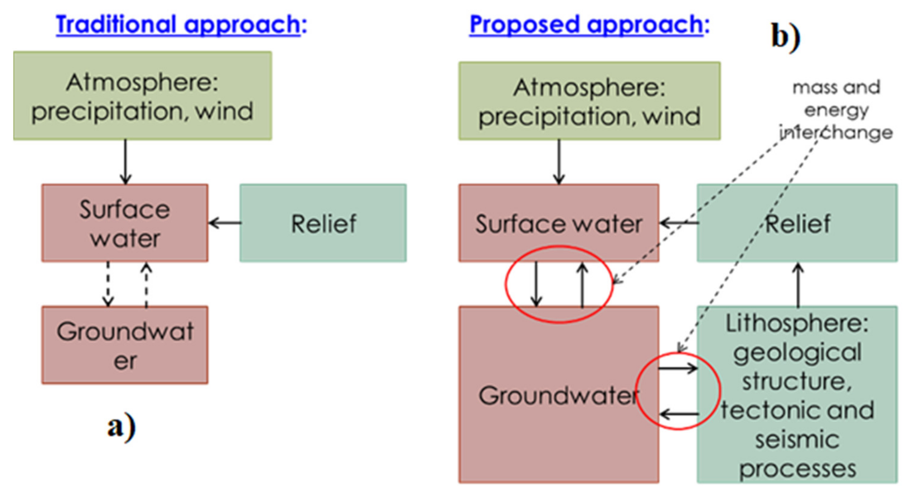
- All water is formed from precipitation according to the local terrain;
- (2)
- Surface water is considered separately from groundwater during any event.
2. Methods
2.1. Basic Concept of General Approach
- (1)
- Precipitation in a specific, selected area and its level estimation in quantitative parameters;
- (2)
- Discharge and water flow processes along the river bed, and related measurements that were carried out;
- (3)
- Groundwater distribution with regard to its volume and lifecycle by monitoring their state at the time.
2.2. Database and Complex Analysis
- (1)
- Only disastrous/historical events (for observing the extremes of considered parameters);
- (2)
- No coastal regions (excluding tsunamis);
- (3)
- No seasonal events (excluding freshets);
- (4)
- Acceptable spatial and temporal lags—not more than a month.
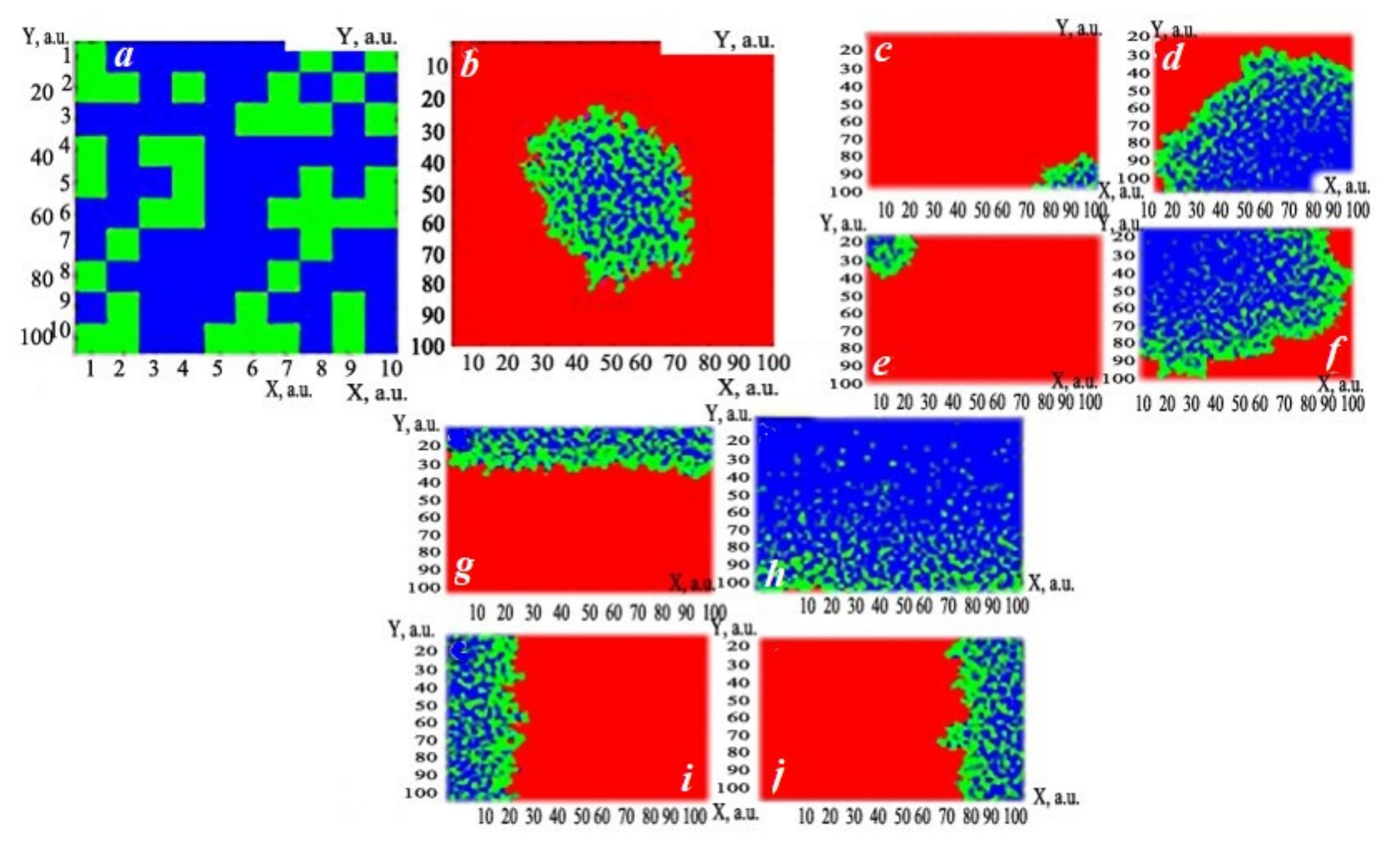
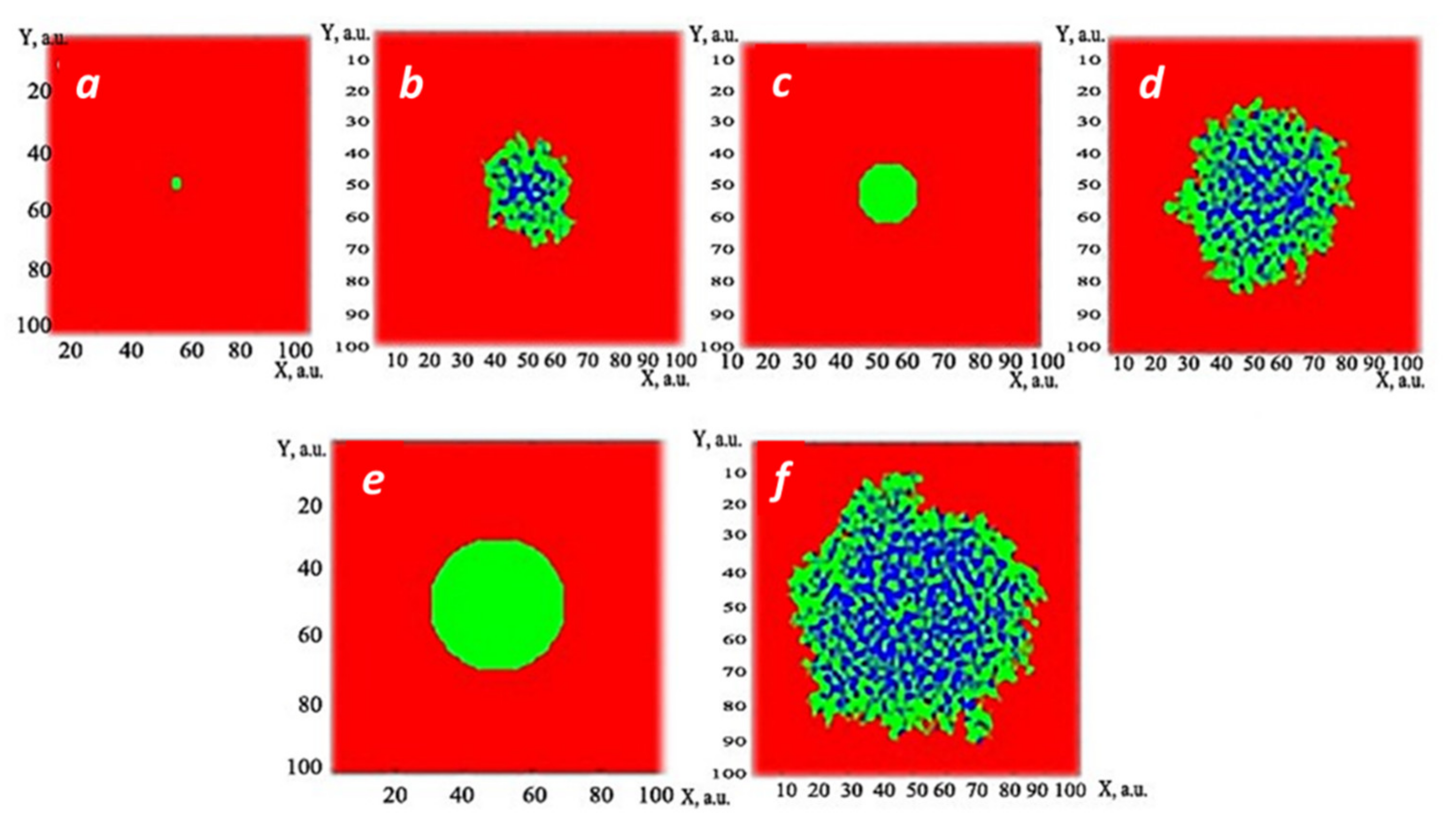
2.3. Dynamic Models and Reconstruction of 3D-Crack-Net under External Factors
- (1)
- The basis was crack fractal modeling in the rock structure;
- (2)
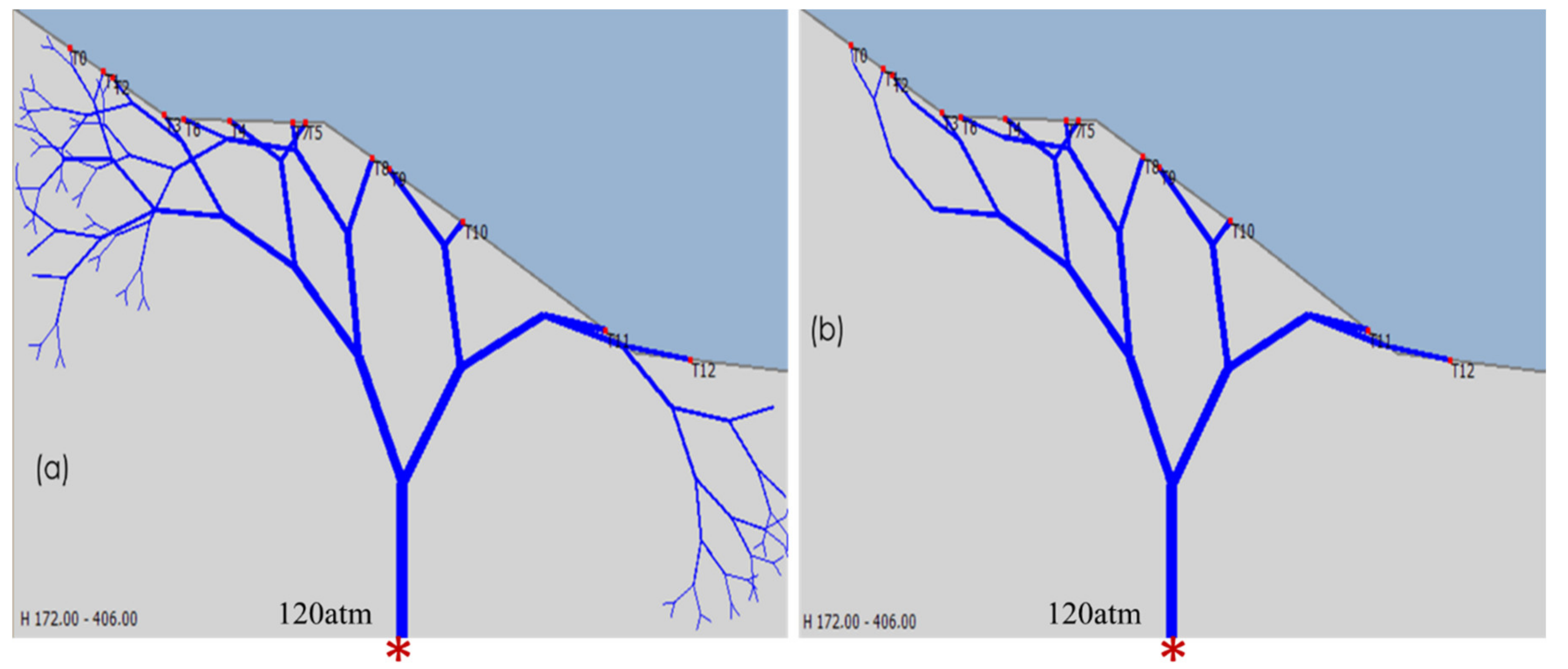
- Cracks were superimposed on the earth surface profile where points of crack emergence on the surface were formed.
- (3)
- It was assumed that the entire crack network was filled with water;
- (4)
- The pressure in the head fracture was set, and the computer algorithm calculated what pressures would be at the emergence points of different surface exits;
- (5)
- Excluded cracks not coming to the surface and could create a tension zone inside the rocks.
3. Results
3.1. Statistical Analysis
- Independence/coherence/steady state of each process development according to its internal laws, as determined by autocorrelation function;
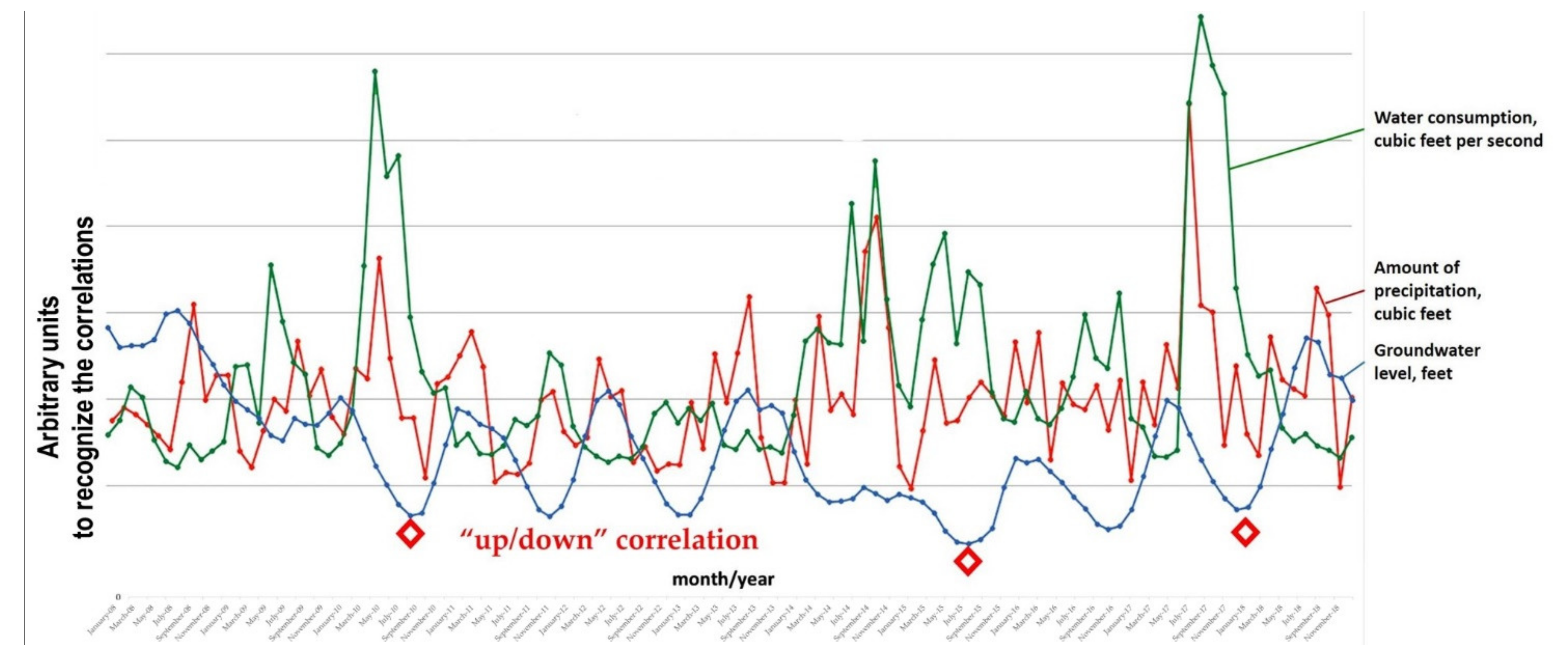
- The processes of correlation and mutual interaction being demonstrated in pair/crossed combinations;
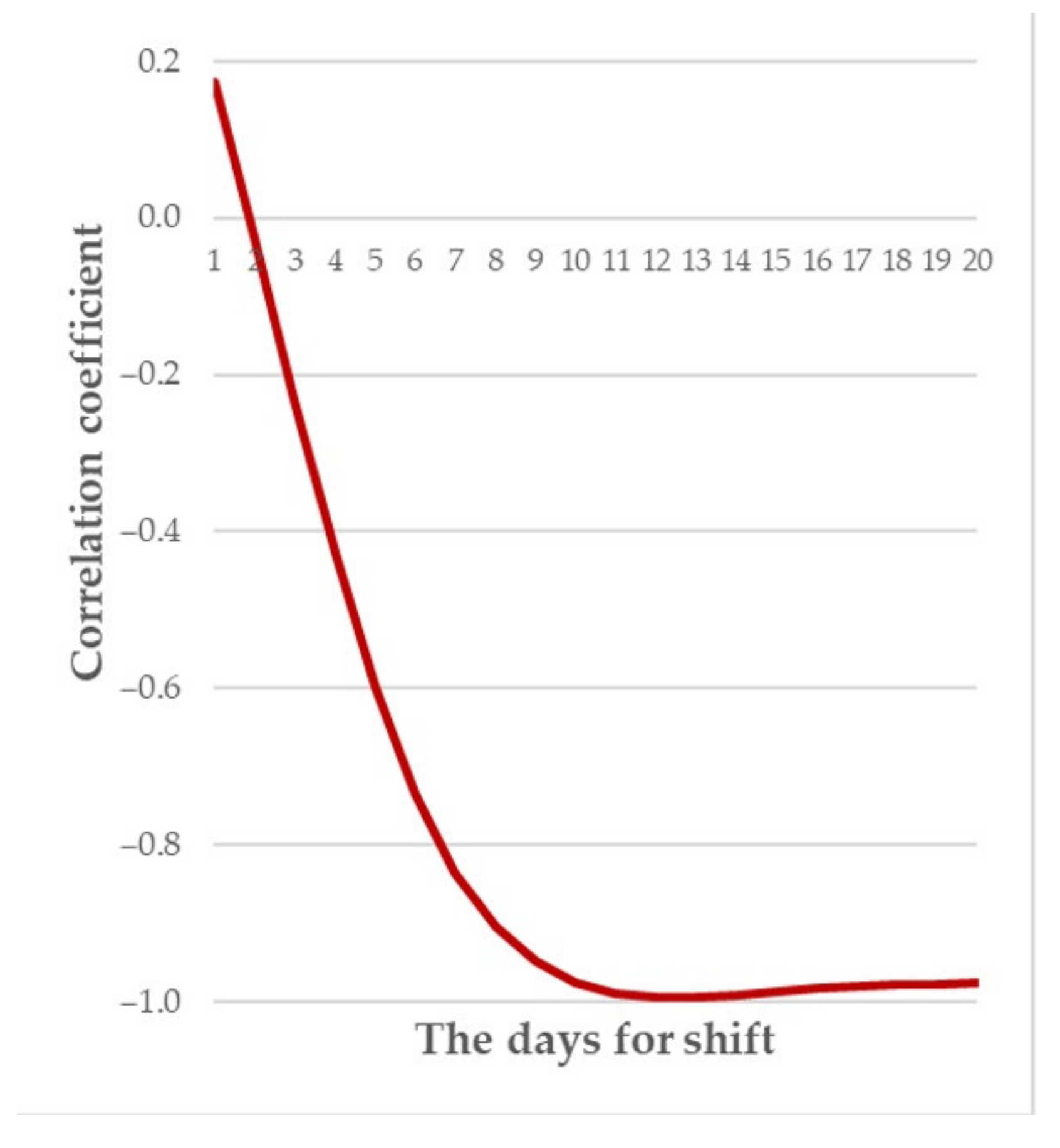
- The same correlations but with different time shifts due to obvious and reasonable delays between different processes by selecting optimal time-shift as an adjustable parameter;
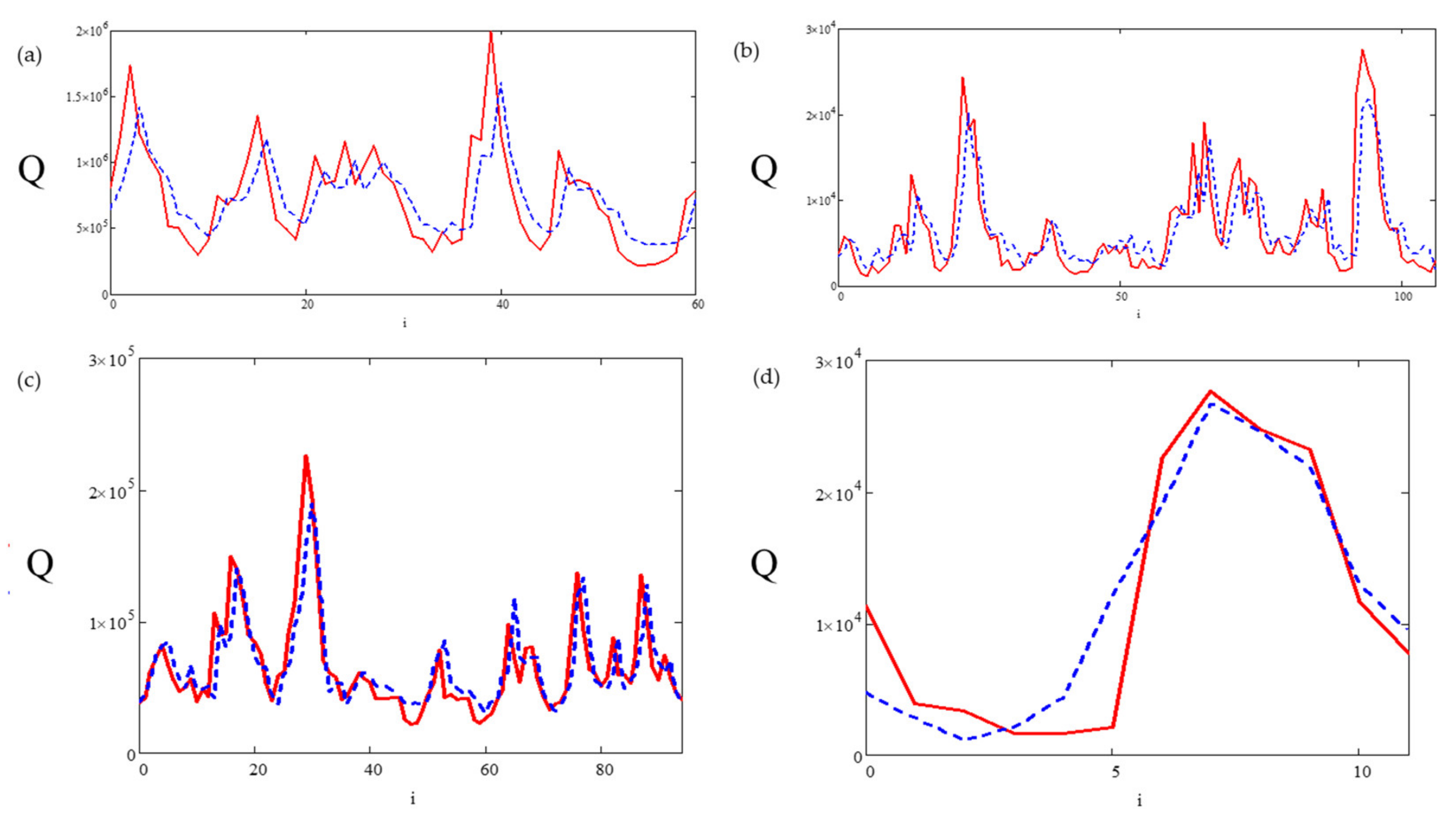
- Forecasting procedure with predictable parameters in time for the studied processes based on known/measured initial/fixed values.
- (i)
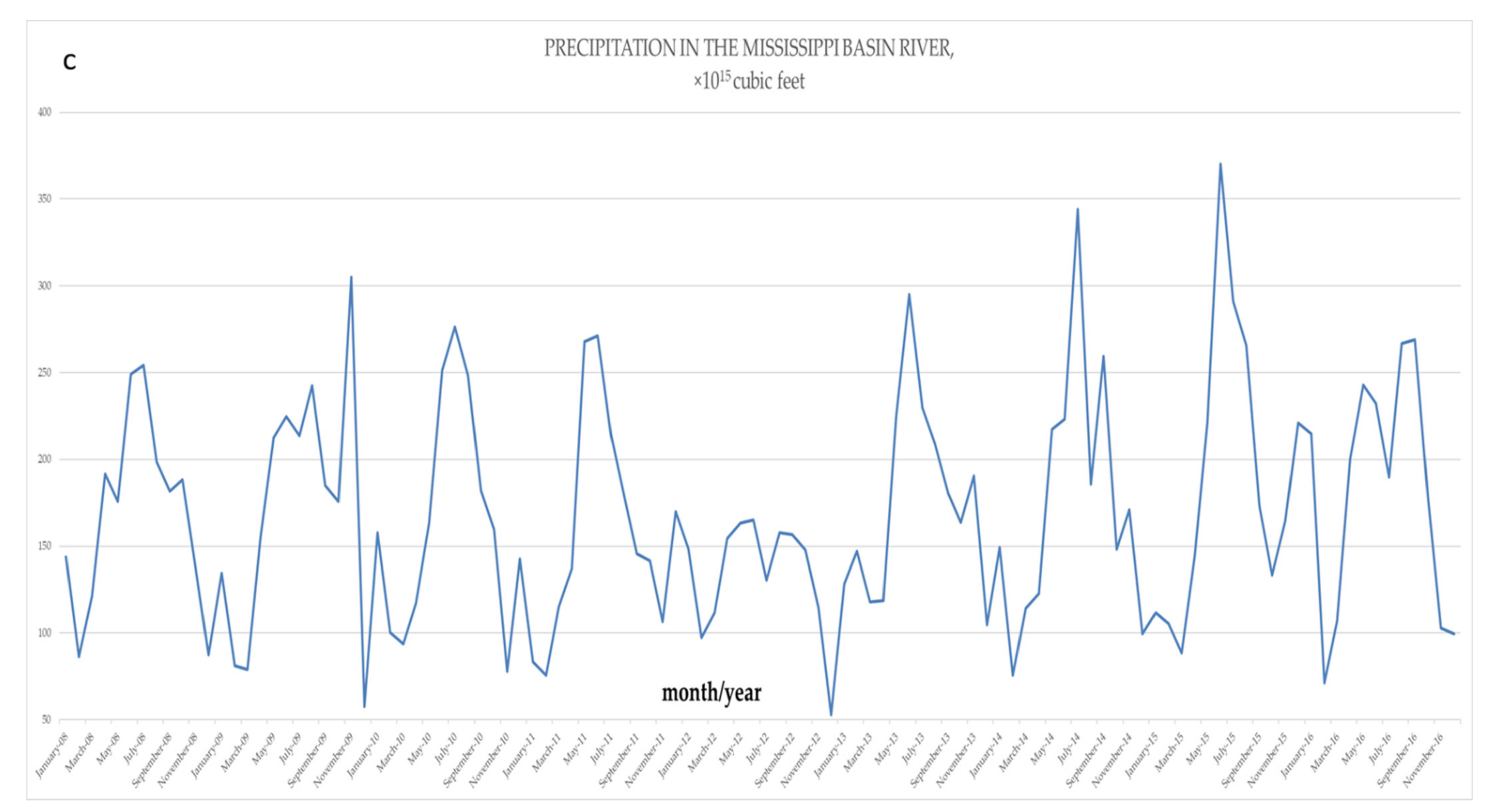
- Discharge and precipitation—are under season variations;
- (ii)
- Groundwater—relatively speaking, is not directly correlated to season specifies;
- (iii)
- Correlations/anticorrelations—do exist for such parameters as discharge mass, groundwater state and precipitation level.
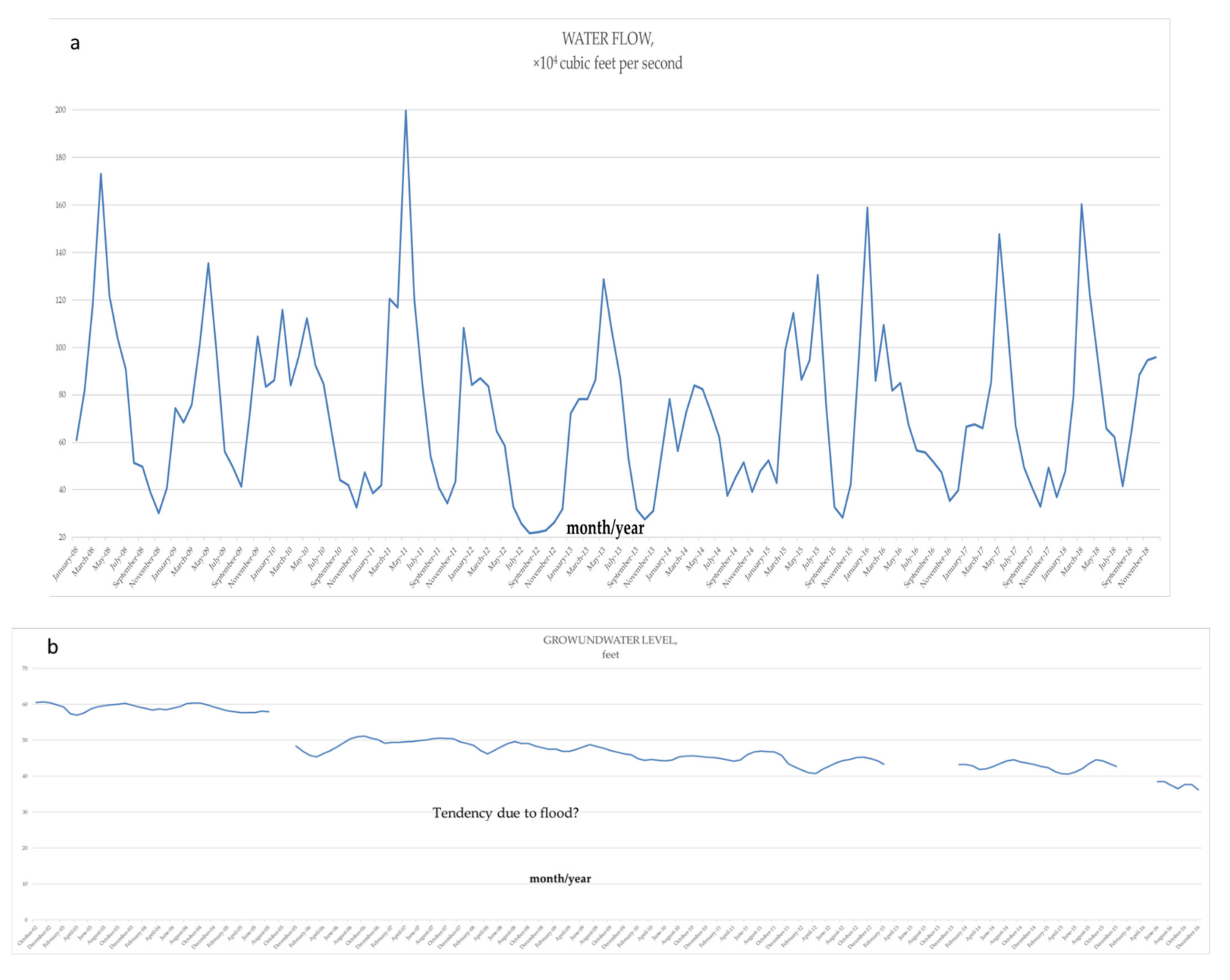
- (1)
- During catastrophic floods: the peak correlation of both precipitation (the Mississippi/Missouri region (no flooding simultaneously)) and discharge (on July 2011) were observed, but, as for groundwater level, the process of downfall occurs only in a single month (August 2011), and it has not recovered even in 2 years.
- (2)
- As to autocorrelations for each unit: Strong for groundwater but weak for both precipitation and discharge take place.
- (3)
- For mutual/pair correlations in a more detailed analysis we received:
- Negative correlation/anticorrelation coupling for groundwater and discharge in general, but it did not couple directly during the flood;
- Positive correlation coupling for precipitation and discharge but with some variations in time;
- No direct correlation coupling for groundwater and precipitation at the same time interval.
- (4)
- We recognized a pair correlation of the processes with a temporal shift (±over several months) and did optimization by searching for the maximal correlation for the river basins: 1 month for the Mississippi and the Missouri, but 3 months for Santee.
- (5)
- Regressive multifactor analysis was carried out with 0.33% accuracy for local data in comparison with averaging all data.
3.2. Earthquake Impact
4. Discussion
5. Conclusions
- Based on the discussed model, forecasts with vital information about both groundwater hydrostatic/hydrodynamic pressure distribution and water flows, carried out by a water crack 3D map in mountain massifs, should be introduced into theory and analysis.
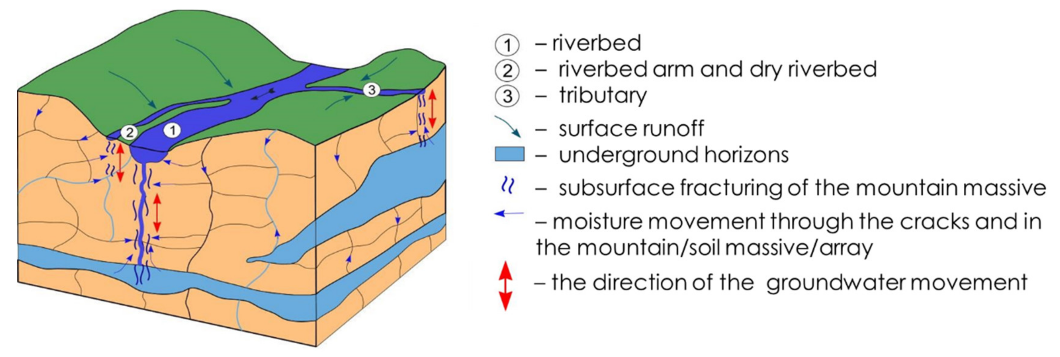
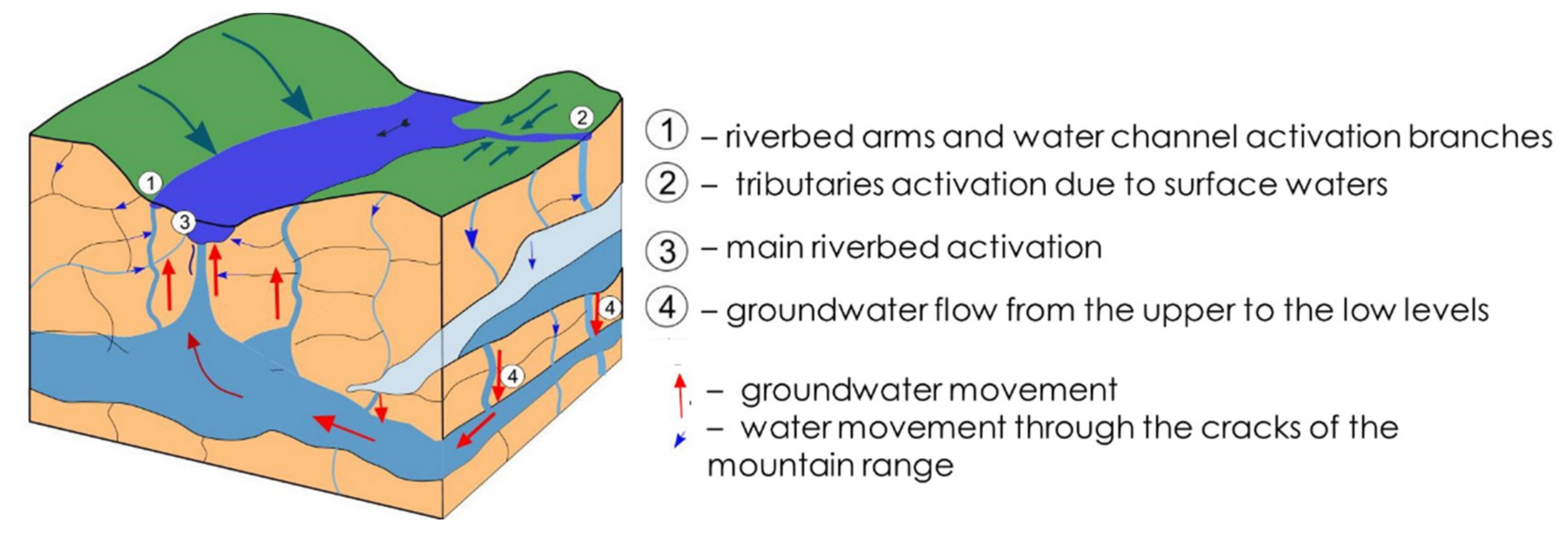
- A necessary condition for the dramatic development of the phenomena is the breaking down of impermeable rock caused by sudden openings in crack-ways (previously blocked), that become active for some reason; e.g., due to shower runoff impact, geo-thermal stream influence, or earthquakes.
- The water from the top hill-lake/reservoir and/or down-lake/reservoir (local base level) can reach the below and/or upper river area (the base level) via the activated groundwater transportation routes due to connecting vessels affected by the development of a backwater process because of intrinsic pressure variation.
- Traditional and artesian wells, being preliminary and artificially made by a certain topology strategy, bring up an opportunity to formulate water cracks with hydrostatic/hydrodynamic pressures in the 3D map of the mountain massif; i.e., a recognition of the water flow physical state for modeling. This approach results in knowledge of real parameters for modeling and, finally, for a forecast map design taking into account the necessary databases by satisfying the greatest challenges for acceptable risk estimation and early warning systems.
- (1)
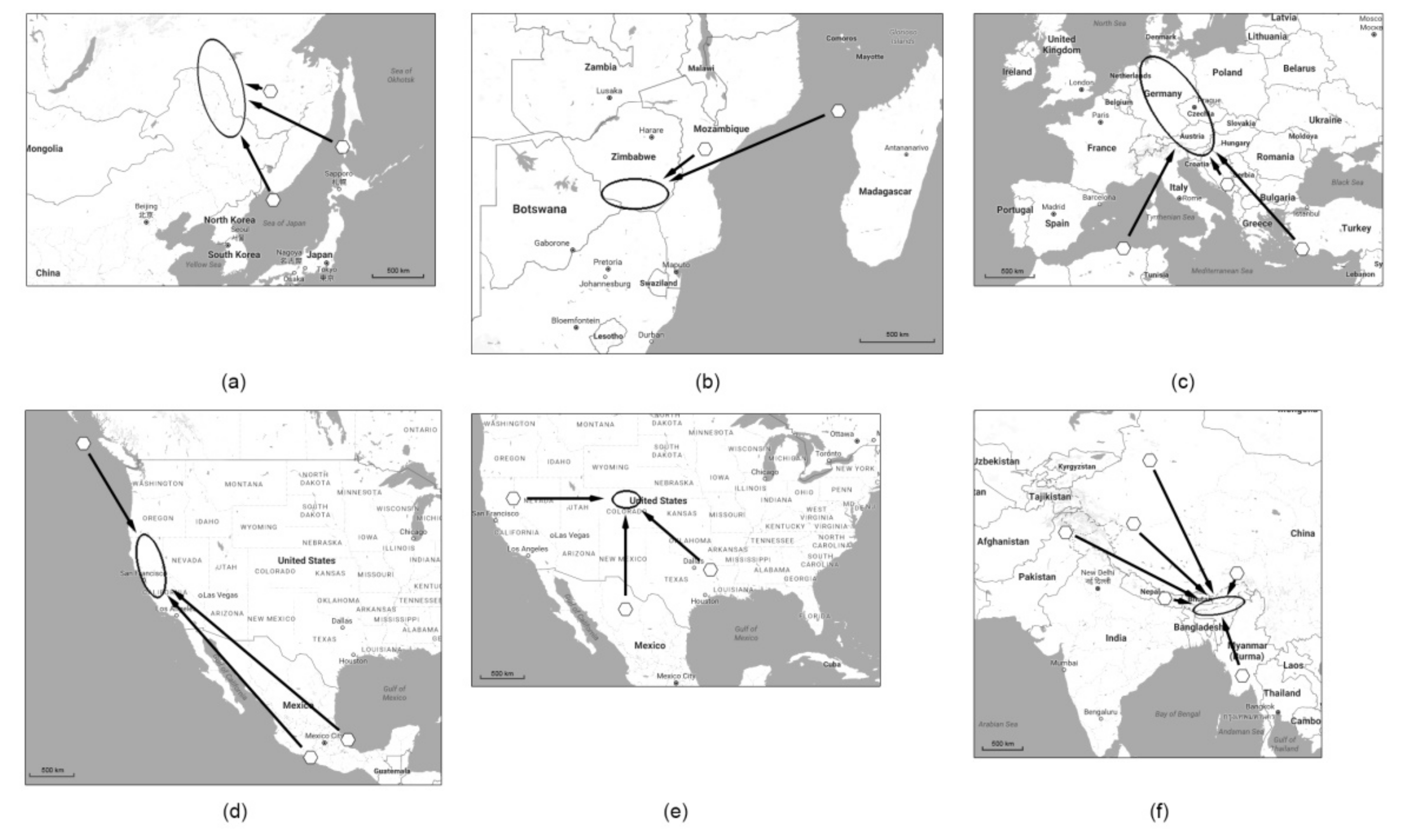
- One-directional arrangement: it can be both a single earthquake and a group of earthquakes.
- (2)
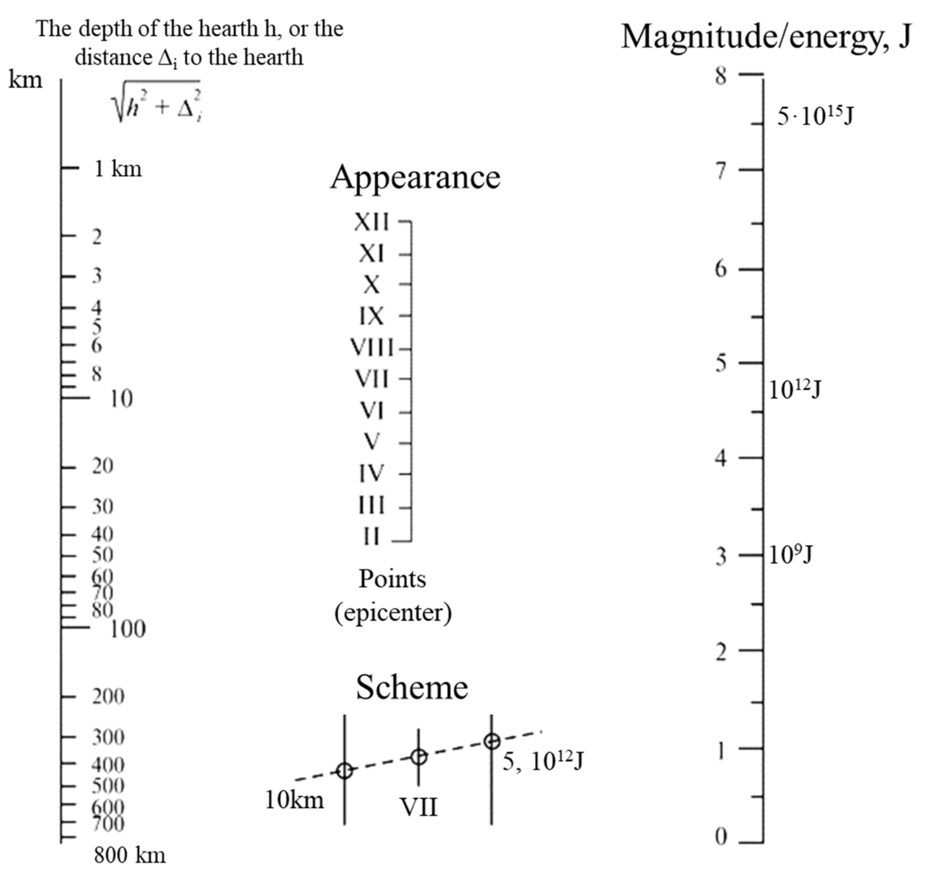
- Two-directional arrangement: the general case is the arrangement of epicenter groups at different distances and directions from the risk zone; in this case, an additional analysis of local geological structures and groundwater recharge rates is necessary (the example of a special case is the arrangement of epicenter groups at equal distances from the risk zone).
- (3)
- Multi-directional arrangement from any earthquake source.
- (1)
- Blockage of some parts with dramatic pressure rises in the net with a water-hammer manifestation on the surface.
- (2)
- Connection/disconnection of groundwater basins (smoother development of flood; longer effect of flow).
- (1)
- Local restructuring of 3D-transport-net topology that does not break the stable regime of river basin functionality.
- (2)
- Significant restructuring of the 3D-transport-net topology that breaks the stable regime of the river basin’s functionality and causing the water level to rise in the river, resulting in the flood.
- (3)
- Significant restructuring of the river’s 3D-transport-net topology that affects the common, unified groundwater basin, e.g., for two rivers, and causing a catastrophic rise in the water level in the river (for one surface river basin) and a fall in water level in the river (for another neighboring surface river basin).
Author Contributions
Funding
Informed Consent Statement
Conflicts of Interest
Appendix A

- 2.
- If we talk about liquid/groundwater movement in cracks with a small cross-section, the speed of such movement strongly depends on fractured rock composition, which leads to a paradoxical result where a more viscous mixture has higher velocity (see [53,54,55]). This issue with hydrodynamics and related phenomena (see [1,2,3,17,34,56]) requires separate consideration for each specific underlying surface case, in association with the discharge and debris processes.
References
- Jakob, M.; Hungr, O. Debris-Flow Hazards and Related Phenomena; Springer Science: Berlin, Germany, 2005; p. 745. [Google Scholar]
- Davies, T.R.H. Large debris flows: A macro-viscous phenomenon. Acta Mechanica. 1986, 63, 161–178. [Google Scholar] [CrossRef]
- Bimal, K.P. Environmental Hazards and Disasters: Contexts, Perspectives and Management; Waley–VCH Verlag GmbH&Co. KGA.: Hoboken, NJ, USA, 2011; 334p. [Google Scholar]
- Caers, J. Modeling Uncertainty in the Earth Science; Waley–VCH Verlag GmbH&Co. KGA.: Hoboken, NJ, USA, 2011; 246p. [Google Scholar]
- Holden, J. (Ed.) An Introduction to Physical Geography and the Environment, 3rd ed.; Pearson Edu. Lim.: Harlow, UK, 2012; 875p. [Google Scholar]
- Flooding Recedes in Europe, but Death Toll Rises and Questions Mount. Available online: https://www.nytimes.com/live/2021/07/17/world/europe-flooding-germany (accessed on 22 February 2022).
- USGS Water Resources: National Water Information System: Web Interface. Available online: https://waterdata.usgs.gov/nwis/dv?referred_module=sw&search_criteria=state_cd&search_criteria=site_tp_cd&submitted_form=introduction (accessed on 22 February 2022).
- Trifonova, T.; Trifonov, D.; Arakelian, S. The 2015 disastrous floods in Assam, India, and Louisiana, USA: Water balance estimation. Hydrology 2016, 3, 41. [Google Scholar] [CrossRef]
- America’s Watershed Initiative Report Card for the Mississippi River. 4 December 2015; 80p. Available online: https://americaswatershed.org/2015-report-card/ (accessed on 22 February 2022).
- National Center for Environmental Information: Storm Events Database. Available online: https://www.ncdc.noaa.gov/stormevents/choosedates.jsp?statefips=-999%2CALL (accessed on 22 February 2022).
- National Water Information System: Mapper. Available online: https://maps.waterdata.usgs.gov/mapper/index.html (accessed on 22 February 2022).
- Europe Flooding Deaths Pass 125, and Scientists See Fingerprints of Climate Change. Available online: https://www.nytimes.com/live/2021/07/16/world/europe-flooding-germany (accessed on 22 February 2022).
- Trifonova, T.; Arakelian, S.; Trifonov, D.; Abrakhin, S.; Koneshov, V.; Nikolaev, A.; Arakelian, M. Nonlinear Hydrodynamics and Numerical Analysis for a Series of Catastrophic Floods/Debris (2011–2017): The Tectonic Wave Processes Possible Impact on Surface Water and Groundwater Flows. In New Trends in Nonlinear Dynamics. Proceedings of the First International Nonlinear Dynamics Conference (NODYCON 2019), Rome, Italy, 17–20 February 2019; Springer: Berlin/Heidelberg, Germany, 2020; Volume 3, pp. 213–222. [Google Scholar]
- Images Related to Flooding in Eastern Russia. Available online: https://earthobservatory.nasa.gov/images/related/81941/flooding-in-eastern-russia (accessed on 22 February 2022).
- Traffic on Trans-Siberian Railway Halted after Bridge Collapse. Available online: https://www.euronews.com/2021/07/23/traffic-on-trans-siberian-railway-halted-after-bridge-collapse (accessed on 22 February 2022).
- Trifonova, T.A. River catchment basin as a self-organizing natural geosystem. Izvestia RAS. Geogr. Ser. 2008, 1, 28–36. [Google Scholar]
- Stein, S.; Wysession, M. An Introduction to Seismology, Earthquakes and Earth Structure; Blackwell: Oxford, UK, 2003; 511p. [Google Scholar]
- Fifth Fatality Feared, More Than 200 Unaccounted For As Colorado Floods Force More Evacuations. Available online: https://www.businessinsider.com/fifth-fatality-feared-more-than-200-unaccounted-for-as-colorado-floods-force-more-evacuations-2013-9 (accessed on 22 February 2022).
- World-wide Hydrogeological Mapping and Assessment Programme (WHYMAP). Available online: https://www.whymap.org/whymap/EN/Home/whymap_node.html (accessed on 18 January 2022).
- Nelson, J.M.N. An Introduction to River Modelling—A Multidimensional Approach; Waley–VCH Verlag GmbH&Co. NYP: Hoboken, NJ, USA, 2012. [Google Scholar]
- Trifonova, T.; Trifonov, D.; Bukharov, D.; Abrakhin, S.; Arakelian, M.; Arakelian, S. Global and regional aspects for genesis of catastrophic floods: The problems of forecasting and estimation for mass and water balance (surface water and groundwater contribution). In Flood Impact Mitigation and Resilience Enhancement; IntechOpen: London, UK, 2020; p. 190. [Google Scholar]
- Jaeger, J.; Cook, N.; Zimmerman, R. Fundamental of Rock Mechanics; Waley–VCH Verlag GmbH&Co. KGA.: Hoboken, NJ, USA, 2007; 475p. [Google Scholar]
- Safonova, N.V. To Zeno’s aporias. Scientific notes of the Crimean Federal University named after VI Vernadsky Philosophy. Political Science. Culturology 2018, 4, 65–73. Available online: https://cyberleninka.ru/article/n/k-aporiyam-zenona (accessed on 22 December 2021).
- Alwin, S. Nonlinear Science: Emergence and Dynamics of Coherent Structures, 2nd ed.; Oxford University Press: Oxford, UK, 2003. [Google Scholar]
- National Weather Service: Advanced Hydrologic Prediction Service. Available online: https://water.weather.gov/precip/ (accessed on 22 February 2022).
- Global Incident Map. Available online: http://quakes.globalincidentmap.com/ (accessed on 18 January 2022).
- Maximilian, J.W.; Kayo, I.; Didier, S. Earthquake forecasts based on data assimilation sequential. Monte Carlo methods for renewal point processes. Nonlin. Processes Geophys. 2011, 18, 49–70. [Google Scholar]
- Jiménez, A.; Posadas, A.M.; Marfil, J.M. A probabilistic seismic hazard model based on cellular automata and information theory. Nonlinear Processes in Geophysics, European Geosciences Union (EGU). Nonlin. Processes Geophys. 2005, 12, 381–396. [Google Scholar] [CrossRef]
- Li, M.; Yang, F.; Zhang, T. Study on Simulation of Foreshock Activity Properties before Strong Earthquake Using Heterogeneous Cellular Automata Models. Int. J. Geosci. 2014, 5, 274–285. [Google Scholar] [CrossRef][Green Version]
- Zheng, Y.; Cao, J.X.; He, X.Y. Study of the time-evolution of underground rock fractal permeability after the earthquakes. Chin. J. Geophys. 2018, 61, 4126–4135. [Google Scholar] [CrossRef]
- Jammu Rain Wonder. A geological phenomenon in the Indian State of Haryana (21.07.2021). Available online: https://youtu.be/rNLDSBY3lXQ (accessed on 22 February 2022).
- Kerzhentsev, A.S.; Meisner, R.; Demidov, V.V. Modeling of Erosion Processes in the Territory of a Small Catchment Basin; Nauka: Moscow, Russia, 2006; 224p. [Google Scholar]
- Global Earthquakes Map. Available online: https://earthquake.usgs.gov/earthquakes/map/ (accessed on 22 February 2022).
- González, P.; Tiampo, K.; Palano, M. The 2011 Lorca earthquake slip distribution controlled by groundwater crustal unloading. Nat. Geosci. 2012, 5, 821–825. [Google Scholar] [CrossRef]
- The USGS Earthquake Hazard Program of the US Geological Survey (USGS). Available online: https://earthquake.usgs.gov/ (accessed on 22 February 2022).
- 2017, U.S. Billion-dollar Weather and Climate Disasters: A Historic Year in Context. Available online: https://www.climate.gov/disasters-2017 (accessed on 22 February 2022).
- Shpakova, R.; Kusatov, K.; Mustafin, S.; Trifonov, A. Changes in the Nature of Long-Term Fluctuations of Water Flow in the Subarctic Region of Yakutia: A Global Warming Perspective. Geosciences 2019, 9, 287. [Google Scholar] [CrossRef]
- The Water Level in the Ob River Has Approached Record Lows. Available online: https://novos.mk.ru/social/2021/09/10/uroven-vody-v-obi-priblizilsya-k-rekordno-nizkim-pokazatelyam.html (accessed on 22 February 2022).
- De Blij, H.J.; Muller, P.O.; Burt, J.E.; Mason, J.A. Physical Geography: The Global Environment; Oxford University Press: Oxford, MA, USA, 2013; 626p. [Google Scholar]
- Weatherley, D.K.; Henley, R.W. Flash vaporization during earth quakes evidence by gold deposits. Nature Geoscience 2013, 6, 294–298. [Google Scholar] [CrossRef]
- Google Maps. Available online: https://www.google.com/maps (accessed on 7 July 2016).
- Allatra.GeoCenter.info. Information and Analytical Portal. Available online: https://geocenter.info/ (accessed on 27 December 2021).
- Shiklomanov, I. World Freshwater Resources. In Water in Crisis: A Guide to World Freshwater Resources; Peter, H.G., Ed.; Oxford University Press: Oxford, MA, USA, 1993; 24p. [Google Scholar]
- Louisiana Topographic Maps by Topo Zone. Available online: http://www.topozone.com/louisiana/ (accessed on 7 July 2016).
- National Weather Center. Available online: http://www.cpc.ncep.noaa.gov/products/Soilmst_Monitoring/US/US_Soil-Moisture-Monthly.php (accessed on 27 December 2021).
- Shebalin, N.V. Foci of strong earthquakes on the territory of the USSR. In USSR Academy of Sciences; Schmidt, O.Y., Ed.; Institute of Physics of the Earth; Nauka: Moscow, Russia, 1974. [Google Scholar]
- Neukom, R.; Steiger, N.; Gómez-Navarro, J.J. No evidence for globally coherent warm and cold periods over the preindustrial Common Era. Nature 2019, 571, 550–554. [Google Scholar] [CrossRef] [PubMed]
- Bliznecov, M. The Frequency of Warming and Cooling on Earth. Available online: https://proza.ru/2020/05/31/1571 (accessed on 27 December 2021).
- Yew, C.H.; Weng, X. Mechanics of Hydraulic Fracturing, 2nd ed.; Elsevier Inc.: Amsterdam, The Netherlands, 2014; p. 470. [Google Scholar]
- Hendriks, M.R. Introduction to Physical Hydrology; Oxford University Press: Oxford, MA, USA, 2010; p. 352. [Google Scholar]
- Gudmundsson, A. Rock Fractures in Geological Processes; Cambridge University Press: Cambridge, MA, USA, 2011. [Google Scholar] [CrossRef]
- Christakos, G. Stochastic Environmental Research and Risk Assessment (SERRA); Springer: Berlin/Heidelberg, Germany, 2015; Volume 29, pp. 637–652. [Google Scholar]
- Maja, V.; Backholm, M.; Timonen, J.V.I.; Ras, R.H.A. Viscosity-enhanced droplet motion in sealed superhydrophobic capillaries. Sci. Adv. 2020, 6, eaba5197. [Google Scholar] [CrossRef]
- De Padova, D. Analysis of the artificial viscosity in the smoothed particle hydrodynamics modelling of regular waves. J. Hydraul. Res. 2014, 52, 836–848. [Google Scholar] [CrossRef]
- Alexandro, V.A. Generation of surface fluid flow in channels by capillary vibrations and waves. J. Technol. Phys. 2022, 92, 194–208. [Google Scholar]
- Trifonova, T.A. The role of groundwater in floods and mudflows. In Nature (Russia); Nauka: Moscow, Russia, 2013; pp. 13–19. [Google Scholar]
- The Kol’skaya super-deep. Investigation of the Deep Structure of the Continental Crust by Drilling the Kola Ultra-Deep Well; Kozlovsky, E.A., Ed.; Nedra: Moscow, Russia, 1984; p. 490, UDC: 622.241 (470.22). [Google Scholar]
- Snir, O.; Friedler, E.; Ostfeld, A. Optimizing the Control of Decentralized Rainwater Harvesting Systems for Reducing Urban Drainage Flows. Water 2022, 14, 571. [Google Scholar] [CrossRef]
- Trifonova, T.A.; Akimov, V.A.; Arakelian, S.M.; Abrakhin, S.I.; Prokoshev, V.G. Fundamentals of Modeling and Forecasting of Natural and Man-Made Emergencies. Comprehensive Analysis of the Development of Fundamental Natural Processes in the Earth’s Crust Using Modern Mathematical Methods and Information Technologies; All-Russian Research Institute of Civil Defense and Emergency Situations (Federal Center): Moscow, Russia, 2014; 436p. [Google Scholar]
- Debris|NASA. Available online: https://www.nasa.gov/centers/hq/library/find/bibliographies/space_debris (accessed on 13 January 2022).
- Preziosi, E.; Rotiroti, M.; Condesso de Melo, T.M.; Hinsby, K. Natural Background Levels in Groundwater; MDPI: Geneva, Switzerland, 2022; 192p. [Google Scholar] [CrossRef]


| Earthquake Location | Geographical Coordinates of Epicenter | Date | Magnitude | Depth of Hypocenter | Flood Location | Flooding Period | River Basin |
|---|---|---|---|---|---|---|---|
| Montenegro | 43.15° N 18.86° E | 21 May 2013 22:55 | 4.5 | 10 km | Germany Czech Republic Austria | May–June 2013 | Danube Elbe |
| Bosnia and Herzegovina | 43.81° N 17.05° E | 20 May 2013 9:24 | 4.0 | 10 km | |||
| Algeria | 36.85° N 5.10° E | 19 May 2013 9:07 | 5.1 | 10 km | |||
| Muğla Province, Turkey | 36.96° N 28.49° E | 16 May 2013 3:02 | 5.0 | 10 km | |||
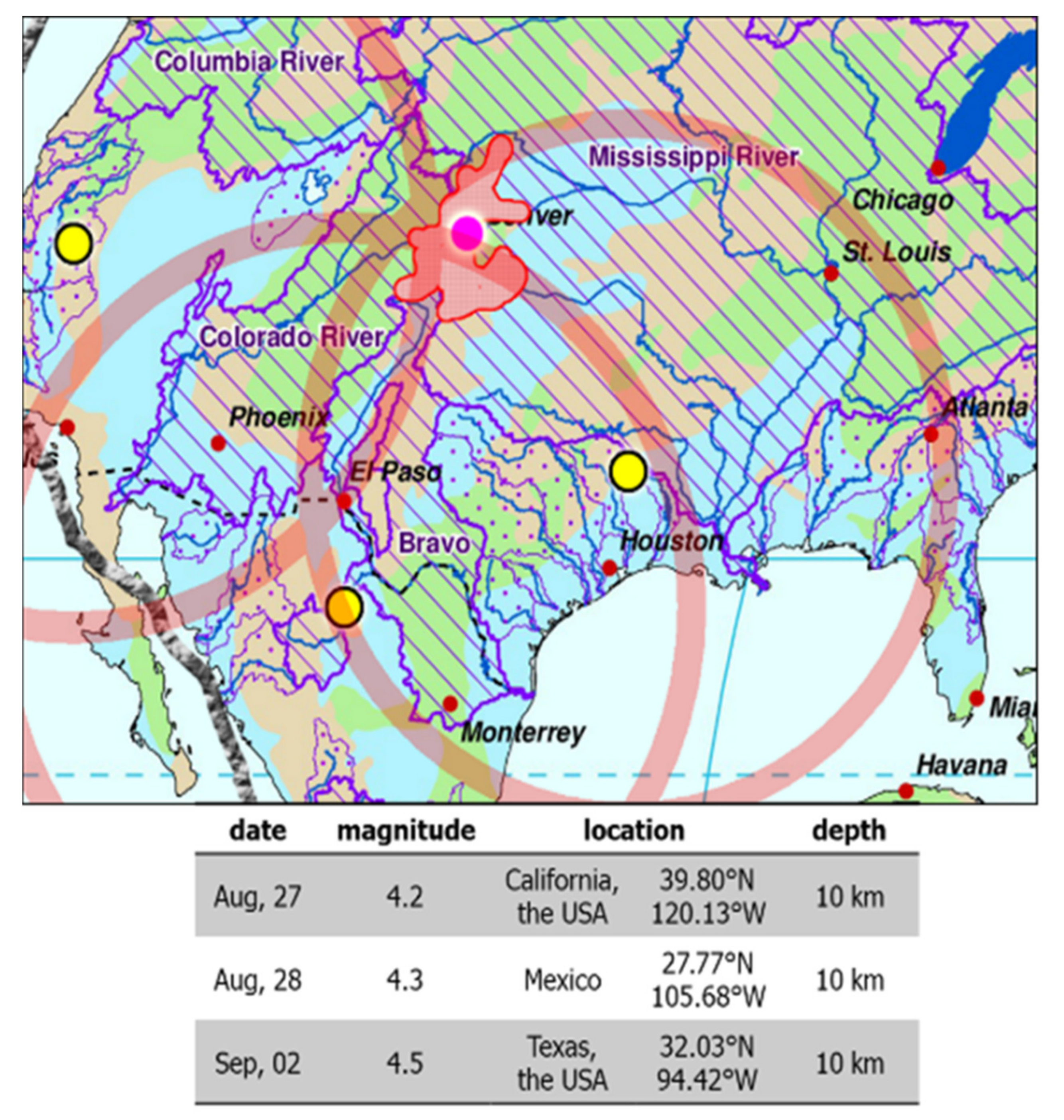
| Texas, USA | 32.03° N 94.42° W | 2 September 2013 23:51 | 4.5 | 10 km | Colorado, USA | September 2013 | Boulder |
| Mexico | 27.77° N 105.68° W | 28 August 2013 20:29 | 4.3 | 10 km | |||
| California, USA | 39.80° N 120.13° W | 27 August 2013 0:51 | 4.2 | 10 km | |||
| Kansas, USA | 37.52° N 98.74° W | 23 May 2015 18:44 | 4.0 | 10 km | Louisiana, USA | June 2015 | Red River |
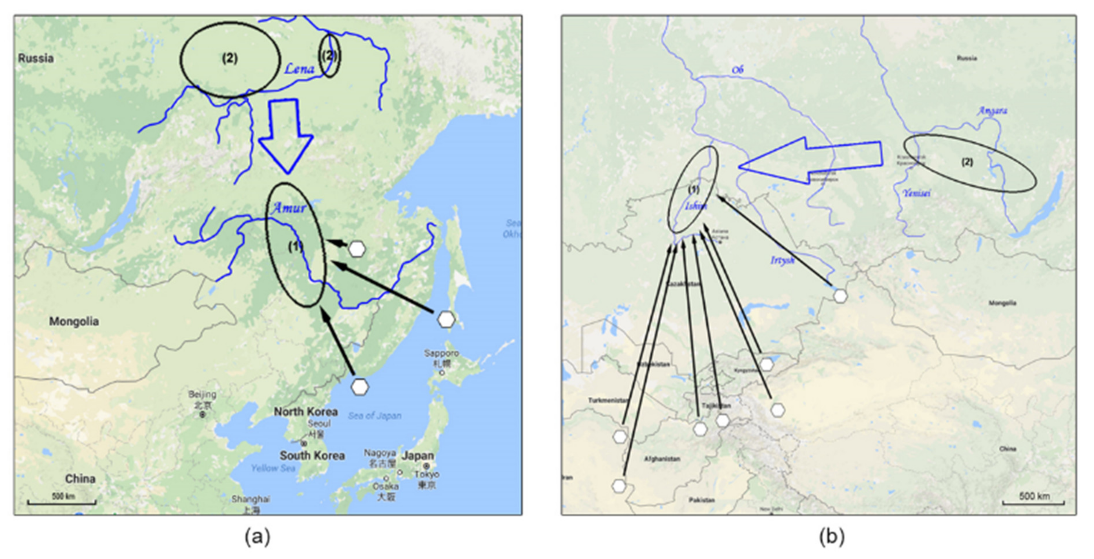
| Kyrgyzstan | 41.93° N 76.80° E | 28 April 2017 5:01 | 4.7 | 10 km | Kazakhstan Tyumen oblast, Russia | April–May 2017 | Ishim |
| Xinjiang, China | 37.88° N 78.13° E | 20 April 2017 3:39 | 4.6 | 10 km | |||
| Afghanistan | 36.51° N 70.93° E 36.70° N 71.51° E 36.42° N 69.17° E | 17 April 2017 23:04 4 April 2017 4:48 2 April 2017 2:48 | 5.0 4.8 4.8 | 184 km 167 km 46 km | |||
| Tajikistan | 37.76° N 72.19° E | 10 April 2017 6:57 | 4.8 | 110 km | |||
| Iran | 35.73° N 60.42° E 31.23° N 60.43° E | 5 April 2017 6:09 4 April 2017 0:12 | 6.1 4.5 | 15 km 10 km | |||
| Kazakhstan | 47.19° N 85.06° E | 4 April 2017 15:07 | 5.1 | 10 km | |||
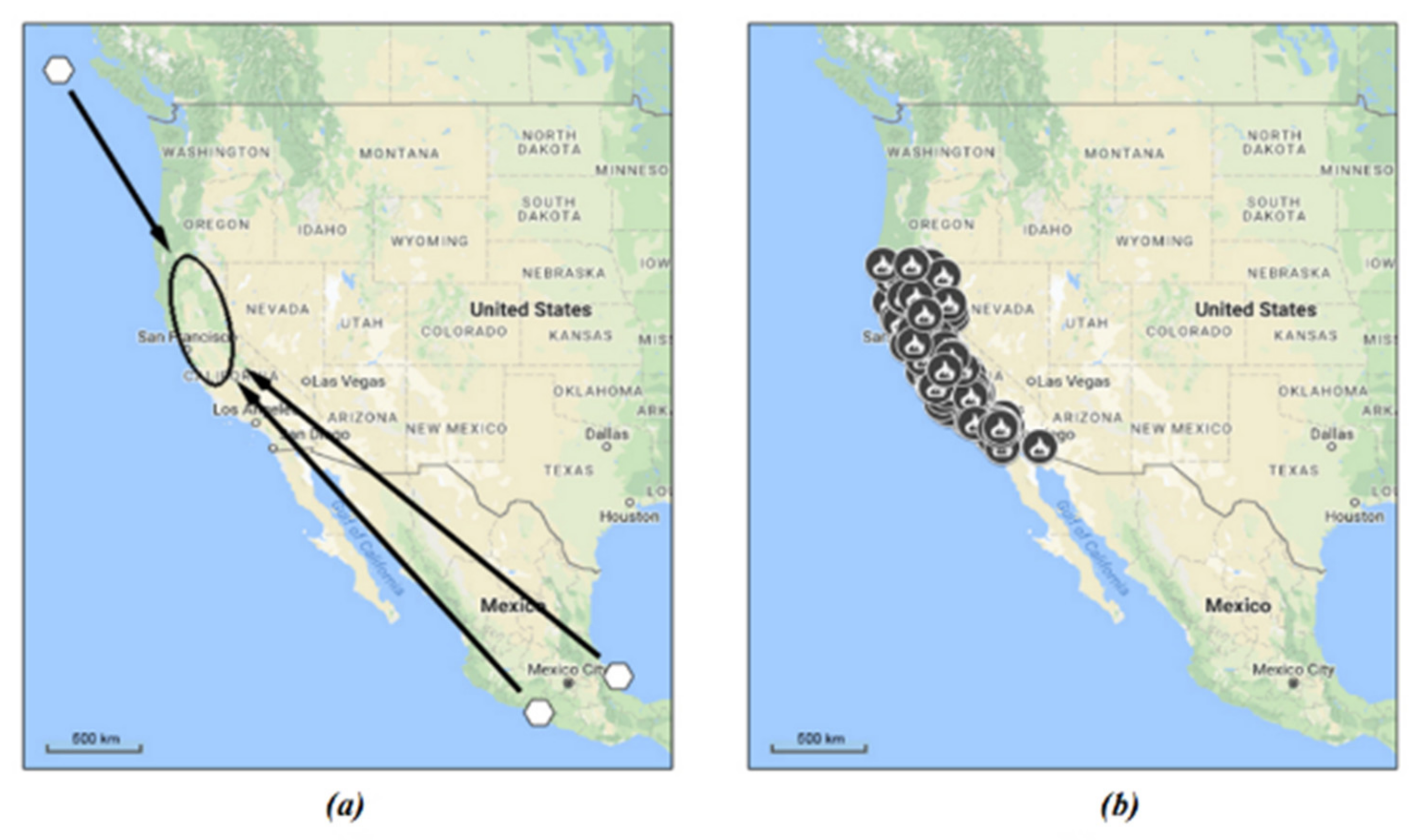
| Mexico | 19.62° N 95.90° W 17.21° N 99.54° W 17.60° N 100.97° W 17.87° N 94.40° W 16.79° N 98.26° W 16.26° N 98.75° W | 15 February 2017 9:56 13 February 2017 7:29 2 February 2017 0:52 25 January 2017 20:54 12 January 2017 10:26 7 January 2017 6:16 | 4.4 4.7 4.7 4.9 5.0 4.6 | 32 km 34 km 23 km 179 km 39 km 10 km | California, USA | February–June 2017 | Sacramento |
| Vancouver Island, Canada | 49.38° N 129.30° W 49.92° N 127.60° W 50.22° N 129.95° W | 12 February 2017 3:47 31 January 2017 1:38 6 January 2017 15:49 | 4.7 4.1 5.3 | 10 km 10 km 10 km |
| River | γ for Water Flow (Discharge) | γ for the Ground Water Level | γ for Precipitation |
|---|---|---|---|
| Mississippi (May 2011) | 0.89118678 | 0.271321887 | 0.857674013 |
| Boulder Creek (September 2013) | 0.996339325 | 0.220981998 | - |
| Santee (October 2015) | 0.959963899 | 0.547425876 | 0.900993342 |
| Missouri (2011) | 0.901901813 | 0.653395031 | 0.857674013 |
| Items | Selected Collection of Seismic Events/ and Data/and Magnitude | Proposed Related Flood/ and Data | Time Factor/ Time Delay for Coupling | Distance between Two Events (Coupling Scale) | Note |
|---|---|---|---|---|---|
| I. Basic events/test events for establishment of the coupling | |||||
| 1. | Nord Japan/ 26 April 2001/5.96 | Lensk (Yakutiya, Russia)/ 14 May 2001 | 18 days | 2.2∙103 km | (1) artesian cracknet with spatial distance of groundwater coupling—about few thousand km (2) sudden modification of the 3D-crack topology and resistance against the fluid flows |
| 2. | Nord Taiwan/ 14 June 2001/5.87 | Kultuki (Irkutsk region, Russia)/7 July 2001 | 23 days | 3.4∙103 km | |
| 3 | Afghanistan/ 3 January 2002/6.05 | Temruke (Krasnodar region, Russia)/ 10 January 2002 | 7 days | 2.9∙103 km | |
| II. Verification of the proposed coupling (events at present) | |||||
| 4. | Popocatepetl Volcanic eruption (Mexico)/ 5 July 2013 | Ruyaya State (Mexico)/20 July 2013 | 15 days | 1.3∙103 km | Should be the flashy flow process due to the ground pressure sudden enhancement ~1000 atm |
| 5. | (a) Instability Land Cluster in time: Sakuradzima Volcanic eruption (Kyushu island, Japan)/ 10 July 2013/ emission of ash from the volcano up to 3 km height; (b) Izu Archipelago (Japan)/ 11 July 2013/ 5.3; (c) Nord-East Honshu island (Japan)/ 13 July 2013/ 4.5 | Nord Honshu (Japan)/ 18 July 2013 | 5–8 days | 1.9∙103 km 0.9∙103 km 0.2∙103 km | |
| 6. | Kamchatka (Russia)/ 17–18 July 2013; Volcanic Shiveluch/ on July 2013 | Ivanovka (Amur region, Russia)/ 20 July 2013 Kamchatka (Russia)/ 29 July 2013 | 3 days 1–3 days from last eruption | 5.5∙103 km 0.4∙103 km | Continuous Earth-quake vibrations result in 3D-reconstruction of crack-net in continuous dynamics |
| III. Neural-Net training | |||||
| In progress | Needs a reasonable database | ||||
| V. Forecast for acceptable risk | |||||
| In progress | Final goal: The risk mapping design in both space and time | ||||
Publisher’s Note: MDPI stays neutral with regard to jurisdictional claims in published maps and institutional affiliations. |
© 2022 by the authors. Licensee MDPI, Basel, Switzerland. This article is an open access article distributed under the terms and conditions of the Creative Commons Attribution (CC BY) license (https://creativecommons.org/licenses/by/4.0/).
Share and Cite
Trifonova, T.; Arakelian, M.; Bukharov, D.; Abrakhin, S.; Abrakhina, S.; Arakelian, S. Catastrophic Floods in Large River Basins: Surface Water and Groundwater Interaction under Dynamic Complex Natural Processes–Forecasting and Presentation of Flood Consequences. Water 2022, 14, 1405. https://doi.org/10.3390/w14091405
Trifonova T, Arakelian M, Bukharov D, Abrakhin S, Abrakhina S, Arakelian S. Catastrophic Floods in Large River Basins: Surface Water and Groundwater Interaction under Dynamic Complex Natural Processes–Forecasting and Presentation of Flood Consequences. Water. 2022; 14(9):1405. https://doi.org/10.3390/w14091405
Chicago/Turabian StyleTrifonova, Tatiana, Mileta Arakelian, Dmitriy Bukharov, Sergei Abrakhin, Svetlana Abrakhina, and Sergei Arakelian. 2022. "Catastrophic Floods in Large River Basins: Surface Water and Groundwater Interaction under Dynamic Complex Natural Processes–Forecasting and Presentation of Flood Consequences" Water 14, no. 9: 1405. https://doi.org/10.3390/w14091405
APA StyleTrifonova, T., Arakelian, M., Bukharov, D., Abrakhin, S., Abrakhina, S., & Arakelian, S. (2022). Catastrophic Floods in Large River Basins: Surface Water and Groundwater Interaction under Dynamic Complex Natural Processes–Forecasting and Presentation of Flood Consequences. Water, 14(9), 1405. https://doi.org/10.3390/w14091405