Comparison of Marine Ecosystems of Haizhou Bay and Lvsi Fishing Ground in China Based on the Ecopath Model

Abstract

Recently, under the impacts of environmental shifts and human activities, marine ecosystem conservation and recovery have become increasingly important for the management and sustainable development of fishery resources. We construct two Ecopath models to describe and compare the similarities and differences in the structure and function of the ecosystems in Haizhou Bay (HZB) for 2020–2021 and Lvsi Fishing Ground (LSFG) for 2018–2019 in this study. Our results highlight the similarities of the two ecosystems in which plankton (e.g., zooplankton and phytoplankton) are important functional groups with bottom-up effect control and congers control the top-down effect. The differences between the two ecosystems indicate that the HZB ecosystem is relatively mature due to higher Finn’s cycling index (FCI), Finn’s mean path length (FMPL), Connectance Index (CI), System Omnivory Index (SOI), and Ascendency/capacity (A/C). However the food web structure in the LSFG is more diverse and stable with higher Overhead/capacity (O/C) and Overhead/capacity (H). The differences are possibly due to the low trophic level (TL) species composition in the two ecosystems. Therefore, we suggest that stock enhancement and release methods should be deployed to release high TL species into designated water areas to increase food web complexity and ecosystem maturity in HZB and LSFG. This study will help inform ecosystem and fishery regulations in different ways and facilitate discussion towards the establishment of strategic conservation planning and adaptive management.

1. Introduction

The various ecological processes of the marine ecosystem structure are constantly changing in a dynamic balance and are complex and interrelated with temporal and spatial variation [1,2,3]. As an integral part of marine ecosystems, the network structures of the food web can be used to identify the biodiversity, stability and complexity of ecosystems by studying its inner structure, function, and trophic interactions of organisms [4,5]. Generally, Ecopath has been largely applied in generating ecosystem food web models since its initial development in the early 1980s [6,7,8,9]. In particular, it is a fairly mature modeling tool in the study of structures and functions of ecosystems and ecological effects. As well as for evaluating the temporal and spatial diet variations of consumers with different trophic levels in the food webs based mostly on quantitative and new qualitative analysis including diet matrix, biomass, and mortality estimates [10,11,12,13].

Coastal and estuarine ecosystems, which connect land and sea, are crucial transitional zones where energy flow and material exchange among the four spheres (Lithosphere, hydrosphere, atmosphere, and biosphere) of the earth [14,15,16]. Under the influence of the Yellow Sea warm current and its coastal current, Haizhou Bay (HZB) and the Lvsi fishing ground (LSFG) have rich fishery resources and fish species [17,18]. Recently, the increasing fishing intensity and environmental changes have resulted in a decline in economically important species (e.g., Larimichthys polyactis, Collichthys lucidus), as well as its abundance and significant changes in the structure of fishery resources, with the decrease of trophic levels [17]. Since 2002, the local government has begun to build marine protected areas (MPAs) dominated by artificial reefs to restore the ecological environment and protect fishery resources in Haizhou bay [17,19]. In the past, the research in these two regions has mainly focused on biodiversity [20,21], population structure [21], and trophic ecology [18,22]. While food web models are rarely used to describe the structure and function of the ecosystem food web, with the exception of species capacity assessment [23,24] and energy flow analysis [16,17] in these regions.

Given the possible different food web structures in the two fishing grounds, comparisons between different ecosystems can be made to further understand the structures and functions of ecosystems if key ecological indicators that reflect ecosystem characteristics can be identified [16,25]. Our aim is to (1) develop two Ecopath models, one for the HZB ecosystem that incorporates reef species and the other for LSFG ecosystem; and (2) characterize and compare food web structure and function within the two fishing grounds using ecological indicators estimated by the Ecopath model. Our study will explore energy flows and ecosystem maturity in HZB and LSFG to accumulate new data for ecological research in China and provide a scientific fundamental basis for fishery resources utilization and environmental management in the coastal waters.

2. Materials and Methods

2.1. Description of Study Area

2.1.1. Haizhou Bay

HZB is located at the westernmost open bay in the East Yellow Sea (34°45′–35°05′ N, 119°21′–119°29′ E) (Figure 1), with an area of approximately 877 km², which is mainly composed of sandy and muddy habitats [26]. The main fishing operations in this region are trawling and gill-net fishing, and the dominant species are nekton (e.g., L. polyactis and Oratosquilla oratoria). The temperature and hydrology have a significant influence on the mainland of Haizhou Bay, and coastal currents regulate the majority of fishing areas [27]. The main tidal current is a rotating flow with a velocity of 0.4–0.65 m/s and a direction of northeast to southwest [28]. In this region, the average water depth is within 25 m, and the average water temperature and salinity are 19.54 °C and 23.76, respectively [26,27].

2.1.2. Lvsi Fishing Ground

LSFG, an open fishing ground with an area of approximately 30,000 km², which is located at the junction of the East China Sea and East Yellow Sea (32°00′–34°00′ N, 122°30′ E), east of Nantong and Yancheng in Jiangsu Province, north of the Yangtze Estuary, south of Haizhou Bay, and west of the Dasha Fishing Ground (Figure 1). Trawling is the main operation in LSFG, and Larimichthys crocea, Portunus trituberculatus, etc., are the main targeted species in this region. The LSFG is influenced by the Yellow Sea current and the coastline current (the Yangtze river runoff and coastal water masses in northern and central Jiangsu). The average water depth is 29 m, and the average annual surface water temperature and surface salinity are 16.9 °C and 30.8, respectively [20].

2.2. Ecopath Model

The trophic functions and structures of aquatic ecosystems were represented using EwE software (Version 6.5) (from http://www.ecop.org, accessed on 20 December 2021) [8]. Biomass (B), production to biomass ratio (P/B), consumption to biomass ratio (Q/B), and ecotrophic efficiency (EE) were the basic input for each functional group. Diet matrix (consumption and import of food items) for all functional groups were also entered. The basic equation is as follows:

$$B_i{\left(P/B\right)}_{i}E{E}_i=Y_i + B_j{\left(Q/B\right)}_{i}D{C}_{ij} + E_i+B_{i}B{A}_i$$

(1)

where i and j are prey and predator groups, respectively, Y_i is the fishery catch rate, and B_i is the biomass. P/B_i is the ratio of production to biomass of i, Q/B_j is the ratio of consumption to the biomass of predator j, and DC_ji is the matrix of group i in the diet of group j. BA_i is the biomass accumulation and EE_i is the fraction of a group’s total production in a system. System-wide and functional group-specific indices are calculated once a system is balanced. For each functional group in the model, one of the input parameters B, P/B, Q/B, or EE should be left to be estimated [8,29].

With model sizes of 877 km² and 1000 km², two Ecopath models reflecting the status of the HZB and LSFG ecosystems were constructed. Based on carbon sources in the food web and ecological and economic characteristics of major species, we identified 19 ecological functional groups using experimental data from gastric content analysis in the HZB and LSFG ecosystems [17,18].

The input parameters were derived from data during the 2018–2021 fishery resource surveys in HZB and LSFG, fishery statistics, published literature, diet composition reports, and FishBase (www.fishbase.org, accessed on 20 December 2021) [17,18]. The B calculations for most functional groups were based on survey data (HZB in Spring: April 2021, Summer: July 2019, Autumn: September 2020; LSFG in Spring: April 2018, Summer: June 2018, Autumn: October 2018) except for detritus. Q/B were gained from FishBase, and catch, P/B were from survey data and published research [17,30]. To balance the model, the diet matrix, P/B and Q/B of unbalanced functional groups were modified repeatedly to make 0< EE ≤ 1 for each functional group. We also slightly modified B values if models remained unbalanced, as trawl surveys can lead to underestimation [31]. The fishing discards were not included in the analysis and the pre-balance (PREBAL) diagnostics due to the high accuracy of biomass. While the two models were not forced by any environmental parameter (e.g., water temperature and chlorophyll-a).

2.3. Trophic Network Analysis

The indicators of the trophic network analysis, including basic indicators and indicators, which can be used to describe system maturity, were shown in Table 1.

Table 1. Indicators of trophic network analysis.

Indicators		Acronym	Units	Reference
Statistics and flows	Total consumption	Q	t km−2 year−1	[32,33]
	Total exports	Ex	t km−2 year−1
	Flows to detritus	FD	t km−2 year−1
	Total respiration	R	t km−2 year−1
	Total production	P	t km−2 year−1
	Total system throughput	TST	t km−2 year−1
	Total system throughput/TST	Q/TST	–
	Total exports/TST	Ex/TST	–
	Flows to detritus/TST	FD/TST	–
	Total respiration/TST	R/TST	–
	Total production/TST	P/TST	–
	Total biomass/TST	B/TST	–
Ecosystem maturity status	Primary production/total respiration	PP/R	–	[32,34,35,36,37]
	Primary production/total biomass	PP/B	–
	Finn’s cycling index	FCI	%
	Finn’s mean path length	FMPL	%
	System omnivory index	SOI	–
	Connectance index	CI	–
	Ascendency/capacity	A/C	%
	Overhead/capacity	O/C	%
	Shannon diversity index	H	–
Ecosystem efficiency	Mean transfer efficiency	MTE	%	[38]
	MTE from primary production	MTEpp	%
	MTE from detritus	MTEd	%
	Proportion of total flow originating from detritus	PEED	–
Trophic indices	Mean trophic level of the community	MTL	–	[39]
	Marine trophic index	MTL0	–
	High trophic index	HTI	%
	Apex predator indicator	API	%

Table 1. Indicators of trophic network analysis.

Indicators		Acronym	Units	Reference
Statistics and flows	Total consumption	Q	t km−2 year−1	[32,33]
	Total exports	Ex	t km−2 year−1
	Flows to detritus	FD	t km−2 year−1
	Total respiration	R	t km−2 year−1
	Total production	P	t km−2 year−1
	Total system throughput	TST	t km−2 year−1
	Total system throughput/TST	Q/TST	–
	Total exports/TST	Ex/TST	–
	Flows to detritus/TST	FD/TST	–
	Total respiration/TST	R/TST	–
	Total production/TST	P/TST	–
	Total biomass/TST	B/TST	–
Ecosystem maturity status	Primary production/total respiration	PP/R	–	[32,34,35,36,37]
	Primary production/total biomass	PP/B	–
	Finn’s cycling index	FCI	%
	Finn’s mean path length	FMPL	%
	System omnivory index	SOI	–
	Connectance index	CI	–
	Ascendency/capacity	A/C	%
	Overhead/capacity	O/C	%
	Shannon diversity index	H	–
Ecosystem efficiency	Mean transfer efficiency	MTE	%	[38]
	MTE from primary production	MTEpp	%
	MTE from detritus	MTEd	%
	Proportion of total flow originating from detritus	PEED	–
Trophic indices	Mean trophic level of the community	MTL	–	[39]
	Marine trophic index	MTL0	–
	High trophic index	HTI	%
	Apex predator indicator	API	%

2.4. MTI

Ecopath estimated the mixed trophic impact (MTI) by generating a n × n matrix, which estimates the direct and indirect feeding relationships across functional groups in a system [35,40].

2.5. Keystoneness

Keystone and structuring species are two important functional groupings. Keystone species, with low biomass, have a high effect on maintaining the structure and integrity of the food webs [41,42,43]. Structuring species, with high biomass, are defined as predators that have a high effect on the food webs. The equation of keystoneness indices is as follows:

$$K{S}_L = \log \left({\epsilon }_i \times \left(1 - P_i\right)\right) = \log \left(\sqrt{{{\displaystyle \sum }}_{j\ne j}^n{m}_{ij}^2} \times \left(1 - \left(\frac{B_i}{{{\displaystyle \sum }}_k{B}_K}\right)\right)\right)$$

(2)

$$K{S}_V = \log \left(\sqrt{{{\displaystyle \sum }}_{j\ne j}^n{m}_{ij}^2} \times drank\left(B_i\right)\right)$$

(3)

where P_i represents the contribution of functional group i to the total biomass of the food web, and B_i represents the biomass of functional group i. The abbreviation ‘drank’ in Equation (3) represents the rank of a variable, in descending order [43].

3. Results

3.1. Model Parameters (Inputs and Outputs)

Overall, as trophic levels (TLs) increase, the functional group biomass decreases, with species like congers and seabass near the top, and phytoplankton and detritus near the bottom of the flow diagrams (Figure 2). The estimated TLs of the HZB ecosystem model ranged from 1.00 (phytoplankton) to 4.15 (congers), with congers having the highest TLs (>4.00). For the LSFG were from 1.00 (phytoplankton) to 3.27 (congers), with congers and seabass owing the highest TLs (>3.00) (Table 2 and Figure 2). The estimated TLs of most functional groups ranged from 2.00 to 4.00 and from 2.00 to 3.00 in the HZB and LSFG ecosystems, respectively. The EE value in the HZB ecosystem was slightly higher than that in the LSFG ecosystem (Table 2), which indicated that a lower percentage of output flowed of primary producers to detritus.

Table 2. Model parameters for 19 functional groups in two models. Bold represents the basic output. Notes: [30]—Cheng et al., (2010); [17]—Wang et al., (2017); [44]—Li et al., (2010); [23]—Lin et al. (2013); [16]—Ju et al. (2020); “*”—FishBase. (P/B: production-biomass ratio; Q/B: consumption-biomass ratio; TLs: Trophic levels; EE: Ecotrophic Efficiency; P/Q: production-consumption ratio).

HZB	Group Name	Catch (t/km2)	Biomass (t/km2)	P/B (/Year)	Q/B (/Year)	TLs	EE	P/Q (/year)
1	Gobiidae	0.016 [30]	0.366	1.980 [30]	12.117 *	3.674	0.814	0.163
2	Congers	0.207 [30]	0.0592	3.500 [23]	12.000 *	4.145	0.999	0.292
3	Collichthys lucidus	0.008 [6]	0.134	1.658 [30]	7.500 *	3.269	0.989	0.221
4	Larimichthys polyactis	0.008 [6]	0.114	1.658 [30]	7.500 *	3.316	0.965	0.221
5	Other drumfish	0.006 [5]	0.0360	1.067 [23]	6.833 *	3.263	0.988	0.156
6	Seabass	0.003 [17]	0.139	1.058 [30]	4.000 *	3.993	0.728	0.265
7	Sardinella zunasi	0.013 [30]	0.313	3.000 [16]	10.000 [16]	3.221	0.892	0.300
8	Anchovy	0.013 [7]	0.0333	3.000 [23]	16.275 *	2.861	0.848	0.184
9	Filefish	0.100 [30]	0.0446	2.500 [30]	10.800 *	2.912	0.907	0.231
10	Other pelagic fishes	1.097 [30]	0.439	2.600 [30]	9.400 *	2.685	0.964	0.277
11	Benthic fishes	0.035 [30]	0.0530	1.460 [17]	8.650 *	2.471	0.809	0.169
12	Small fishes	0.505 [17]	0.257	2.300 [17]	23.214 *	2.588	0.863	0.099
13	Shrimps	0.400 [17]	1.101	8.000 [17]	28.000 [17]	2.569	0.997	0.286
14	Crabs	0.050 [17]	1.853	3.500 [17]	12.000 [17]	2.867	0.937	0.292
15	Cephalopods	0.400 [17]	0.139	3.000 [17]	10.000 [17]	2.471	0.963	0.300
16	Benthos		0.0435	1.570 [17]	8.600 [17]	2.510	0.891	0.183
17	Zooplankton		2.195	40.000 [17]	160.000 [30]	2.176	0.913	0.250
18	Phytoplankton		26.126	100.000 [17]		1.000	0.064
19	Detritus		80.32 [30]			1.000	0.065
LSFG
1	Gobiidae	0.016 [30]	0.0268	1.980 [30]	16.000 *	2.569	0.783	0.124
2	Congers	0.207 [30]	0.192	2.300 [30]	12.000 *	3.269	0.468	0.192
3	Collichthys lucidus	0.150 [30]	0.102	1.658 [30]	7.500 *	2.894	0.928	0.221
4	Larimichthys polyactis	0.150 [30]	0.353	1.658 [30]	7.500 *	2.793	0.934	0.221
5	Other drumfish	0.281 [30]	0.123	2.392 [30]	10.000 *	2.736	0.969	0.239
6	Seabass	0.003 [30]	0.614	1.058 [30]	4.000 *	3.063	0.360	0.265
7	Sardinella zunasi	0.013 [30]	0.303	0.902 [30]	47.600 *	2.769	0.865	0.019
8	Anchovy	0.288 [30]	0.0573	5.500 [30]	25.000 *	2.623	0.976	0.220
9	Filefish	0.100 [30]	0.0472	2.500 [30]	10.800 *	2.635	0.847	0.231
10	Other pelagic fishes	1.097 [30]	0.454	2.600 [30]	9.400 *	2.501	0.938	0.277
11	Benthic fishes	0.035 [30]	0.0673	1.754 [30]	9.525 *	2.541	0.533	0.184
12	Small fishes	1.097 [30]	0.0410	30.000 [30]	106.300 *	2.486	0.918	0.282
13	Shrimps	1.807 [30]	0.583	7.570 [44]	28.000 [44]	2.544	0.975	0.270
14	Crabs	1.807 [30]	0.906	2.120 [30]	8.180 [44]	2.502	0.976	0.259
15	Cephalopods	0. [30]	0.0716	3.000 [30]	10.000 [30]	2.803	0.927	0.300
16	Benthos		0.00333	5.000 [30]	20.000 [30]	2.100	0.356	0.250
17	Zooplankton		6.532 [30]	40.000 [30]	160.000 [30]	2.000	0.129	0.250
18	Phytoplankton		16.173 [30]	200.000 [30]		1.000	0.295
19	Detritus		83.320 [30]			1.000	0.140

Table 2. Model parameters for 19 functional groups in two models. Bold represents the basic output. Notes: [30]—Cheng et al., (2010); [17]—Wang et al., (2017); [44]—Li et al., (2010); [23]—Lin et al. (2013); [16]—Ju et al. (2020); “*”—FishBase. (P/B: production-biomass ratio; Q/B: consumption-biomass ratio; TLs: Trophic levels; EE: Ecotrophic Efficiency; P/Q: production-consumption ratio).

HZB	Group Name	Catch (t/km2)	Biomass (t/km2)	P/B (/Year)	Q/B (/Year)	TLs	EE	P/Q (/year)
1	Gobiidae	0.016 [30]	0.366	1.980 [30]	12.117 *	3.674	0.814	0.163
2	Congers	0.207 [30]	0.0592	3.500 [23]	12.000 *	4.145	0.999	0.292
3	Collichthys lucidus	0.008 [6]	0.134	1.658 [30]	7.500 *	3.269	0.989	0.221
4	Larimichthys polyactis	0.008 [6]	0.114	1.658 [30]	7.500 *	3.316	0.965	0.221
5	Other drumfish	0.006 [5]	0.0360	1.067 [23]	6.833 *	3.263	0.988	0.156
6	Seabass	0.003 [17]	0.139	1.058 [30]	4.000 *	3.993	0.728	0.265
7	Sardinella zunasi	0.013 [30]	0.313	3.000 [16]	10.000 [16]	3.221	0.892	0.300
8	Anchovy	0.013 [7]	0.0333	3.000 [23]	16.275 *	2.861	0.848	0.184
9	Filefish	0.100 [30]	0.0446	2.500 [30]	10.800 *	2.912	0.907	0.231
10	Other pelagic fishes	1.097 [30]	0.439	2.600 [30]	9.400 *	2.685	0.964	0.277
11	Benthic fishes	0.035 [30]	0.0530	1.460 [17]	8.650 *	2.471	0.809	0.169
12	Small fishes	0.505 [17]	0.257	2.300 [17]	23.214 *	2.588	0.863	0.099
13	Shrimps	0.400 [17]	1.101	8.000 [17]	28.000 [17]	2.569	0.997	0.286
14	Crabs	0.050 [17]	1.853	3.500 [17]	12.000 [17]	2.867	0.937	0.292
15	Cephalopods	0.400 [17]	0.139	3.000 [17]	10.000 [17]	2.471	0.963	0.300
16	Benthos		0.0435	1.570 [17]	8.600 [17]	2.510	0.891	0.183
17	Zooplankton		2.195	40.000 [17]	160.000 [30]	2.176	0.913	0.250
18	Phytoplankton		26.126	100.000 [17]		1.000	0.064
19	Detritus		80.32 [30]			1.000	0.065
LSFG
1	Gobiidae	0.016 [30]	0.0268	1.980 [30]	16.000 *	2.569	0.783	0.124
2	Congers	0.207 [30]	0.192	2.300 [30]	12.000 *	3.269	0.468	0.192
3	Collichthys lucidus	0.150 [30]	0.102	1.658 [30]	7.500 *	2.894	0.928	0.221
4	Larimichthys polyactis	0.150 [30]	0.353	1.658 [30]	7.500 *	2.793	0.934	0.221
5	Other drumfish	0.281 [30]	0.123	2.392 [30]	10.000 *	2.736	0.969	0.239
6	Seabass	0.003 [30]	0.614	1.058 [30]	4.000 *	3.063	0.360	0.265
7	Sardinella zunasi	0.013 [30]	0.303	0.902 [30]	47.600 *	2.769	0.865	0.019
8	Anchovy	0.288 [30]	0.0573	5.500 [30]	25.000 *	2.623	0.976	0.220
9	Filefish	0.100 [30]	0.0472	2.500 [30]	10.800 *	2.635	0.847	0.231
10	Other pelagic fishes	1.097 [30]	0.454	2.600 [30]	9.400 *	2.501	0.938	0.277
11	Benthic fishes	0.035 [30]	0.0673	1.754 [30]	9.525 *	2.541	0.533	0.184
12	Small fishes	1.097 [30]	0.0410	30.000 [30]	106.300 *	2.486	0.918	0.282
13	Shrimps	1.807 [30]	0.583	7.570 [44]	28.000 [44]	2.544	0.975	0.270
14	Crabs	1.807 [30]	0.906	2.120 [30]	8.180 [44]	2.502	0.976	0.259
15	Cephalopods	0. [30]	0.0716	3.000 [30]	10.000 [30]	2.803	0.927	0.300
16	Benthos		0.00333	5.000 [30]	20.000 [30]	2.100	0.356	0.250
17	Zooplankton		6.532 [30]	40.000 [30]	160.000 [30]	2.000	0.129	0.250
18	Phytoplankton		16.173 [30]	200.000 [30]		1.000	0.295
19	Detritus		83.320 [30]			1.000	0.140

Habitat differences and connectivity through sea currents rendered similar species compositions (Table 1, Figure 2) but different main trophic energy flows in the HZB and LSFG ecosystems (Figure 3). In the HZB ecosystem, the distinct functional groups with TLs I-III accounting for more than 98.44% of the overall biomass flows in the system. The TTEs for TLs II to V were 10.11%, 17.53%, 13.98%, and 16.49%, respectively. For the LSFG ecosystem, the distinct functional groups with TLs I-III accounting for more than 99.14% of the total biomass flows in the system. The TTEs for TLs II to IV were 3.59%, 15.5%, and 10.55%, respectively. Overall, the energy flows and TTEs of each TL could reflect the properties of the HZB and LSFG ecosystems.

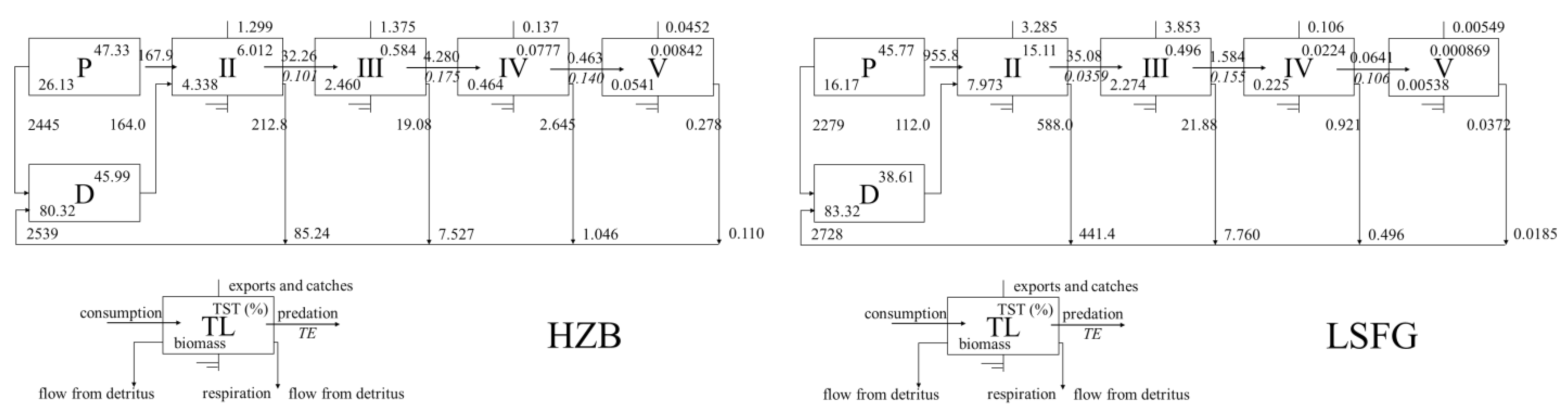
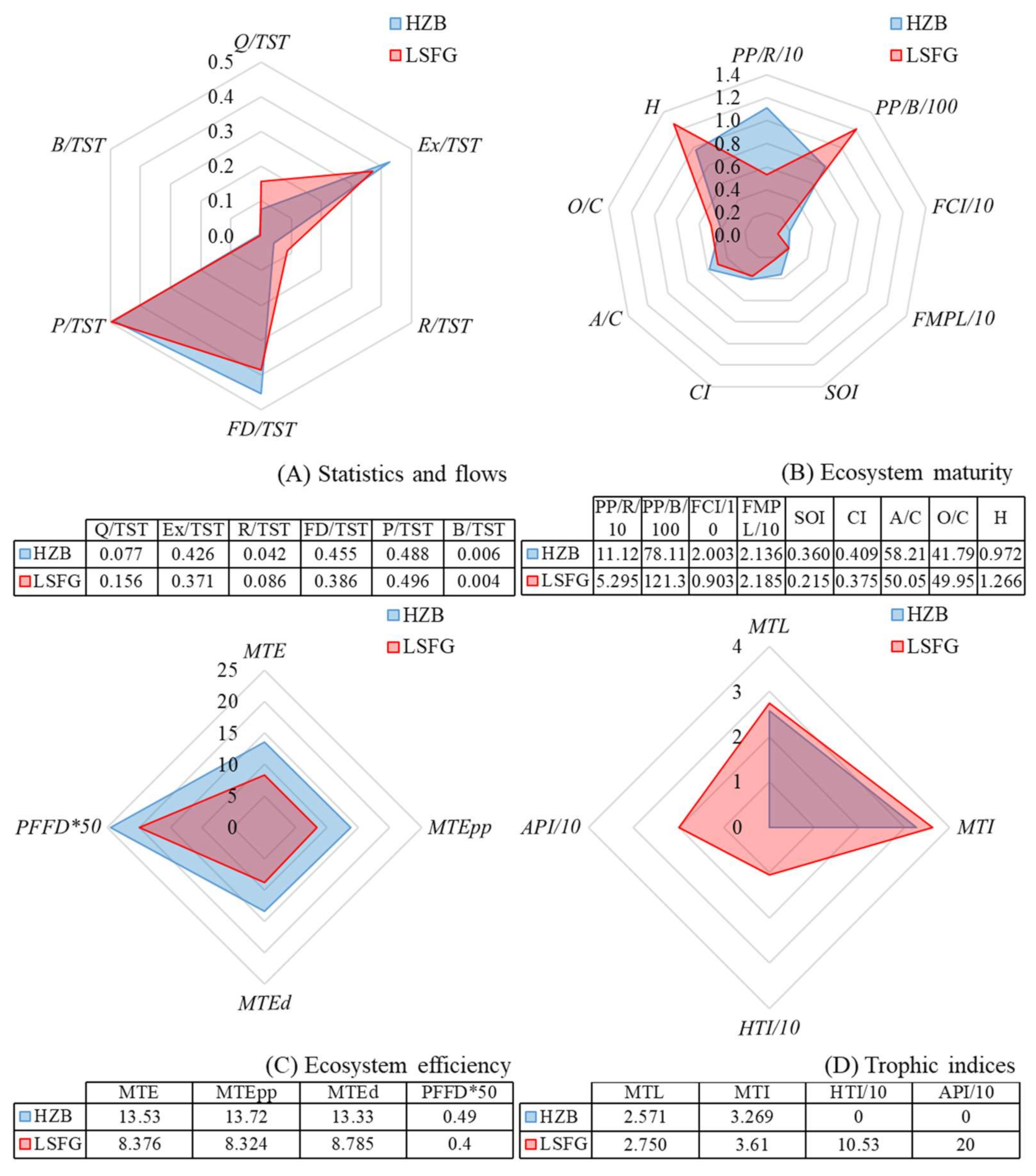
3.2. Properties and Comparison of the HZB and LSFG Ecosystems

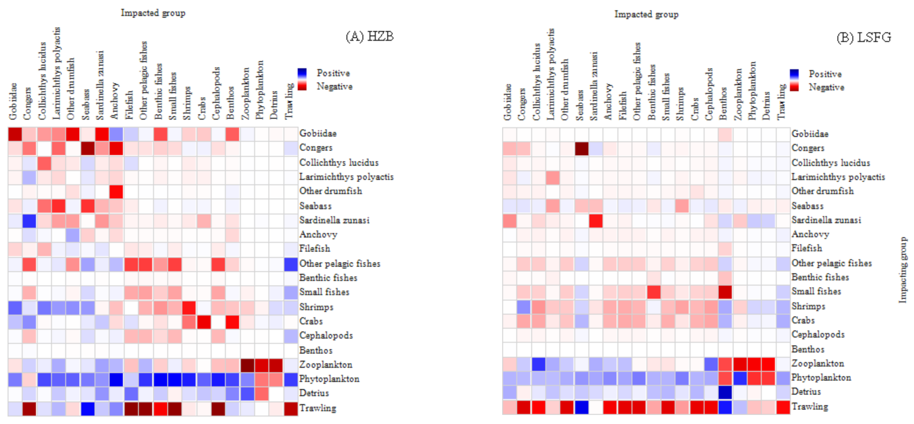
A radial plot was used and visualized to facilitate the comparison of the ecological indicators for the HZB and LSFG ecosystems (Figure 4). As the basic parameters estimated for the HZB ecosystem, the TST was 5580.12 t km⁻² year⁻¹, with percentage contributions of Q (7.68%), EXs (42.61%), R (4.21%) and FD (45.5%). For the LSFG ecosystem, the TST was 7068.207 t km⁻² year⁻¹, of which 15.63% was consumed, 37.12% was exported, 8.64% was respired, and 38.6% flowed to detritus.

With respect to statistics and flows, Ex/TST, FD/TST, and B/TST were all higher or greater in HZB than in LSFG, and other indicators were lower in HZB (Figure 4A). As the ecosystem matured, the values for PP/R, FCI, SOI, CI, and A/C in HZB were higher than those in LSFG, and the remaining indicators were lower in HZB (Figure 4B). The ecosystem efficiency including MTE, MTEpp, MTEd, and PFFD in HZB were higher than those in LSFG (Figure 4C). The MTE in HZB and LSFG was 13.53% and 8.376%, respectively. For HZB, the MTEd food web (13.33%) was lower than that of MTEpp food web (13.72%), but in LSFG, the MTEd (8.785%) was higher than that from MTEpp (8.324%) (Figure 4C). For trophic indices in HZB and LSFG, MTL were 2.75 and 2.571, respectively, and those for MTI₀ were 3.61 and 3.269, respectively (Figure 4D).

3.3. MTI Analysis

MTI analysis reflected that the direct or indirect effects among the functional groups of the ecosystems. It also reflected that trawling fisheries had obvious and direct negative effects on most functional groups in the LSFG ecosystems, and relatively less in the HZB ecosystems (Figure 5). In the HZB ecosystem, Gobiidae, congers, Sardinella zunasi, and plankton had the greatest impact on other functional groups, among which congers had directly negative impact on prey functional groups (e.g., S. zunasi and crabs) and indirectly negative on interspecific competition functional groups (e.g., seabass). However, the benthos and phytoplankton of prey functional groups showed a direct or indirect positive impact. For the LSFG ecosystem, except for shrimps and crabs, the impacts of other functional groups (e.g., Gobiidae, drumfish, and pelagic fishes) were relative. In addition, the phytoplankton of prey functional groups had a direct or indirect positive impact, and the negative effects of high TL groups were more prominent.

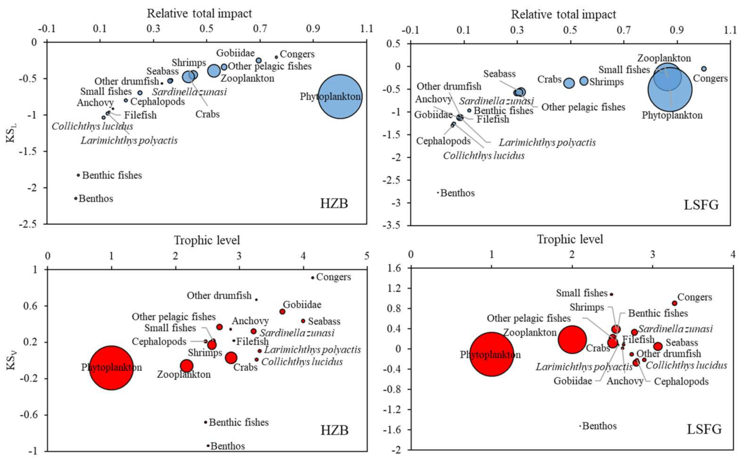
3.4. Keystoneness Analysis

The functional group with the greatest keystoneness index was congers in the HZB ecosystem according to the method by Libralato et al. (2006) (Figure 2). Other groups (e.g., zooplankton, phytoplankton, and Gobiidae) had a high keystoneness index, but they showed higher biomass, especially phytoplankton. Therefore, these groups may be regarded as key structuring groups. Congers were also the highest keystone functional groups, and zooplankton, phytoplankton, small fishes, and shrimp were considered to be structuring groups in the LSFG ecosystem.

The second method used to assess the keystone species ranked two species of top predators (congers and seabass), drumfish and Gobiidae, among the four functional groups with a higher keystoneness in the HZB ecosystem. In the LSFG ecosystem, congers, small fishes, shrimp, and S. dunasi were among the four functional groups with a higher keystoneness. This method confirmed congers as key functional groups and highlighted the importance of top predators in the HZB and LSFG ecosystems. In contrast, both methods ranked other top predators (e.g., congers) and both groups of benthos among the groups with higher keystoneness.

4. Discussion

As a first step towards more effective ecosystem conservation and management plans, the constructed Ecopath food web models can help ecosystem-based approaches for fisheries management. In this study, the similarities and differences in ecosystem structure and function between the HZB and LSFG in China were characterized and compared according to the output data estimated from models. The results of this study can be used to further explore the ecological functions of resource conservation and environmental restoration of two fishing grounds.

4.1. Structure and Function of the HZB and LSFG Ecosystems

The differences of productivity and structure will lead to changes in TST. The results showed that TST of LSFG ecosystem is about 26.7% higher than that of HZB. The reason is that LSFG lies offshore of Jiangsu Province, where the types and forms of seawater impurities are complex and diverse due to water pollution caused by a wide range of human activities (e.g., industrial wastewater discharge, waterway transportation, mariculture), relative to those of HZB [18,20,45], contributing to increased primary productivity. The construction of artificial reefs could increase the biomass of low TL species, enhance productivity, and change the food web structure [46,47]. In the HZB ecosystem, almost all reef species in the sea ranching were extracted as catches (e.g., catches of Sebastiscus marmoratus and Sebastes schlegelii), which led to the lower Q/TST and the greater Ex/TST, thus causing the respiratory consumption and detritus flow of low TL organisms were much higher than those of high TL organisms (Figure 3). Moreover, there were no differences in P/TST (HZB: 0.49; LSFG: 0.5) or B/TST (HZB: 0.006; LSFG: 0.004) between the two ecosystems, which may have been related to similarities in ecosystem type, geological structure, hydrographic conditions, and species composition [16].

Overall, a higher MTE was found in HZB (13.53%) than in LSFG (8.38%), and there was a low TE (0.0359) of TL III groups on TL II groups in LSFG (Figure 3), which may have been related to the high consumption of TL II groups on the primary producers or higher productivity of LSFG (mainly due to the higher biomass, but little flowing to TL III groups of TL II groups). The PFFD in HZB (0.49) was a little higher than that in LSFG (0.4) (Figure 4), because of the higher energy flows of detritus to TL II in HZB (164), as artificial reefs increased the biomass of filter feeders, as well as the flows from detritus [16]. Detritus recycling and the detritus—organisms’ relationship is rather important in the food webs [48,49]. Trophic indices (MTL, MTI₀, HTI, and API) can indicate fishing effects on an ecosystem. The MTL in HZB (2.57) was lower than that in LSFG (2.75) due to the larger numbers of species with low TLs. The HTI and API in HZB were 0 and 10.53 and 20, respectively, for LSFG, possibly because apex consumers prefer more open sea areas, revealing that the fishing pressure and environmental capacity in HZB may be overexploited than LSFG.

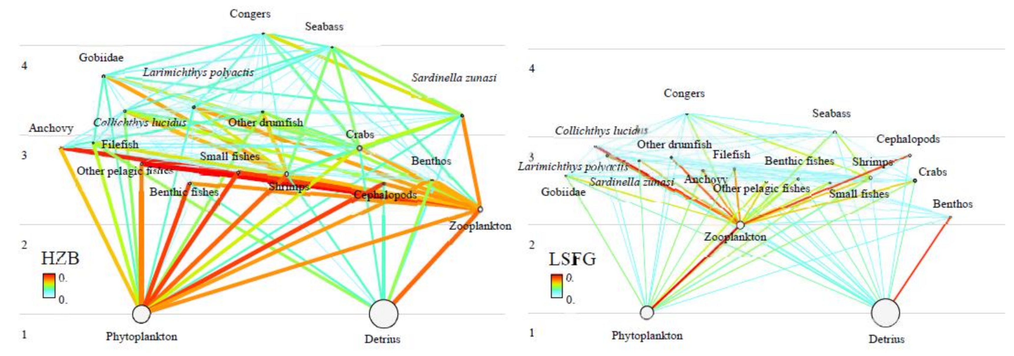
4.2. Trophic Interactions of the HZB and LSFG Ecosystems

In the HZB ecosystem, the biomass of congers had direct negative impacts on prey functional groups (e.g., S. zunasi and crabs) (Figure 5), which means congers are top predators mediating the interaction between functional groups in the food webs in HZB. In the LSFG ecosystem, the abundance of drumfish, anchovies, congers, and other fishes would reduce as shrimp biomass increased. A previous study showed that shrimps, the main food sources of many functional groups, contributed most to the pelagic–benthic coupling on the continental shelf [50], as they exerted high negative effects on high TLs groups through bottom-up effects in the food webs. Moreover, in both ecosystems, phytoplankton and detritus had the largest positive impact, favoring other functional groups as bottom-up controllers; thus, these interactions for policy regulation and fisheries management should be further considered.

The low TL groups—small fishes—were considered to have the highest KS_V in the LSFG ecosystem (Figure 6). In contrast to low-diversity continental shelf ecosystems, which are mostly top-down controlled, species-rich areas are mostly bottom-up controlled [51,52]. The species in LSFG were more diverse than those in HZB based on the Shannon diversity index (H) (LSFG: 1.266 > HZB: 0.972) in this study (Figure 4), which may explain this phenomenon. However, the two methods showed that congers with higher KS_V were important functional groups, and they have negative effects on most functional groups with low TLs, thus impacting the entire food webs, which means that top predators still have a top-down effect in the two ecosystems, but this effect in LSFG may be weaker than that in HZB.

Figure 6. Relative total impact and keystone index values of functional groups in two models. KS_L is from Libralato et al. (2006) [42] and KS_V is from Vall et al. (2015) [43]. Circle size is proportional to biomass.

Figure 6. Relative total impact and keystone index values of functional groups in two models. KS_L is from Libralato et al. (2006) [42] and KS_V is from Vall et al. (2015) [43]. Circle size is proportional to biomass.

4.3. Ecosystem Maturity of the HZB and LSFG Ecosystems

The PP/R ratio is 1 in mature ecosystems but tends to exceed 1 in younger ecosystems [48]. The PP/R ratio in HZB was higher than in LSFG in this study. The primary production of the LSFG ecosystem is mainly from phytoplankton; thus, the PP/R ratio tends to be low. The studies showed that there was a negative correlation between PP/R ratio and PP/B ratio, lower PP/R ratio inevitably resulting in a higher PP/B ratio [34]. The ecosystem in HZB was more mature than that in LSFG with a higher ecosystem maturity index (FCI, FMPL, CI, SOI, and A/C) (Figure 4). This means that in the HZB ecosystem, the energy recycling capability within the system was optimal and strong due to the high FCI, the system structure and the trophic relationship were rich due to the high CI [35], the food web was more complex due to the high SOI, and the degree of specialization was high (20–36%) due to the high A/C ratio, suggesting a relatively more mature and specialized ecosystem [41]. The higher FMPL, CI, and SOI reflect complex inner links and longer trophic pathway in the food webs of mature ecosystems, and the higher O/C value (approximately 19.53% greater than for HZB) suggests a more stable food web in the LSFG ecosystems [53]. In addition, the higher H value in LSFG underlies a relatively immature but more complex and diverse food web in the LSFG ecosystem than in HZB. Generally, relative to the HZB ecosystem, although immature, the food web structure in the LSFG ecosystem is rather diverse and stable.

4.4. Considerations for Assessing Ecosystems through Modelling

The biomass of upper TLs and migratory species has decreased in HZB and LSFG over the last century. Historically abundant top predators (e.g., angler fish or sharks) are now functionally extinct, which exert a considerably diminished impact on ecosystems. This makes congers the most important top predators in both ecosystems in our models. These changes and restructuring of the ecosystem state have been linked to regime shifts, climate variation, predation, and exploitation [54,55,56].

Artificial reefs can reduce the environmental pressure, thus increasing the capacity and stability of marine ecosystems [17,57,58]. Food web complexity, biodiversity, and ecosystem maturity can be enhanced by appropriately increasing the species with high TLs [17,59]. However, we did not see the rich and diverse food web structures in the HZB model. This may be because the modeled area included not only the artificial reef area but also the adjacent waters, which may have contributed to the reduced diversity and complexity of the food web in the HZB ecosystem. In the future, multi-habitat models must be constructed to compare and analyze the energy flow and keystone composition, comprehensively consider the trophic interactions of the food webs in HZB. They must explore the relative merits of the ecosystem structures and functions of sea ranching areas and adjacent waters.

In recent years, stock enhancement and release have been extensively implemented in the coastal waters of China, with high TL species being released into the designated area to increase food web complexity and ecosystem maturity [60]. However, some keystone species (e.g., L. polyactis, C. lucidus) only depend on the bay during some periods of their life history. Therefore, it is urgent to comprehensively understand the biological characteristics of released keystone species and formulate scientific release measures and fishing strategies, and long-term monitoring of fishery management is also needed to ensure sustainable progress. Given that restoring the ecological function of HZB and LSFG ecosystems will not be an easy task, ecological restoration in HZB and LSFG still has a large space for development.

5. Conclusions

In this study, the Ecopath approach provides a good generalization and comparative analysis of ecosystem structure and function in the HZB and LSFG ecosystems. Plankton were identified to be important structuring functional groups with bottom-up effect control, and congers were considered to control the top-down effect in each ecosystem. Overall, the HZB ecosystem is more mature than the LSFG ecosystem due to higher ecosystem maturity status index. However, the food web structure in the LSFG is more diverse and stable with higher O/C and H values. This summary will help inform different ecosystem and fishery regulations in different ways and facilitate discussion towards the establishment of strategic conservation planning and adaptive management.

References

1. Moore, K.J.; Doney, S.C.; Kleypas, J.; Glover, D.; Fung, I.Y. An intermediate complexity marine ecosystem model for the global domain. Deep Sea Res. Part II Top. Stud. Oceanogr. 2001, 49, 403–462. [Google Scholar] [CrossRef] [Green Version]
2. Crowder, L.; Norse, E. Essential ecological insights for marine ecosystem-based management and marine spatial planning. Mar. Policy 2008, 32, 772–778. [Google Scholar] [CrossRef]
3. Heim, K.C.; Thorne, L.H.; Warren, J.D.; Link, J.S.; Nye, J.A. Marine ecosystem indicators are sensitive to ecosystem boundaries and spatial scale. Ecol. Indic. 2021, 125, 107522. [Google Scholar] [CrossRef]
4. Paine, R.T. Food web complexity and species diversity. Am. Nat. 1966, 100, 65–75. [Google Scholar] [CrossRef]
5. Petchey, O.L.; McPhearson, T.; Casey, T.M.; Morin, P.J. Environmental warming alters food-web structure and ecosystem function. Nature 1999, 402, 69–72. [Google Scholar] [CrossRef]
6. Polovina, J.J. Model of a coral reef ecosystem I. The ECOPATH model and its application to french frigate shoals. Coral Reefs 1984, 3, 1–11. [Google Scholar] [CrossRef]
7. Christensen, V.; Pauly, D. ECOPATH II—A software for balancing steady-state ecosystem models and calculating network characteristics. Ecol. Model. 1992, 61, 169–185. [Google Scholar] [CrossRef]
8. Christensen, V.; Walters, C.J.; Pauly, D. Ecopath with Ecosim: A User’s Guide; Fisheries Centre, University of British Columbia: Vancouver, Canada, 2005; Volume 154. [Google Scholar]
9. Taghavimotlagh, S.A.; Vahabnezhad, A.; Shojaei, M.G. A trophic model of the coastal fisheries ecosystem of the northern Persian Gulf using a mass balance Ecopath models. Reg. Stud. Mar. Sci. 2021, 42, 101639. [Google Scholar] [CrossRef]
10. Milessi, A.C.; Danilo, C.; Laura, R.G.; Daniel, C.; Javier, S.; Rodríguez-Gallego, L. Trophic mass-balance model of a subtropical coastal lagoon, including a comparison with a stable isotope analysis of the food-web. Ecol. Model. 2010, 221, 2859–2869. [Google Scholar] [CrossRef]
11. Kong, X.Z.; He, W.; Liu, W.X.; Yang, B. Changes in food web structure and ecosystem functioning of a large, shallow Chinese lake during the 1950s, 1980s and 2000s. Ecol. Model. 2016, 319, 31–41. [Google Scholar] [CrossRef]
12. Lemoine, M.; Moens, T.; Vafeiadou, A.M.; Bezerra, L.A. Resource utilization of puffer fish in a subtropical bay as revealed by stable isotope analysis and food web modeling. Mar. Ecol. Prog. Ser. 2019, 626, 161–175. [Google Scholar] [CrossRef]
13. Han, D.; Tian, S.; Zhang, Y.; Chen, Y. An evaluation of temporal changes in the trophic structure of Gulf of Maine ecosystem. Reg. Stud. Mar. Sci. 2021, 42, 101635. [Google Scholar] [CrossRef]
14. Elliott, M.; Burdon, D.; Hemingway, K.L.; Apitz, S.E. Estuarine, coastal and marine ecosystem restoration: Confusing management and science—A revision of concepts. Estuar. Coast. Shelf Sci. 2007, 74, 349–366. [Google Scholar] [CrossRef]
15. Barbier, E.B.; Hacker, S.D.; Koch, E.W.; Stier, A.C.; Silliman, B.R. Estuarine and coastal ecosystems and their services. Treatise Estuar. Coast. Sci. 2011, 12, 109–127. [Google Scholar] [CrossRef]
16. Ju, P.L.; Cheung, W.W.L.; Chen, M.R.; Xian, W.W.; Yang, S.Y.; Xiao, J.M. Comparing marine ecosystems of Laizhou and Haizhou bays, China, using ecological indicators estimated from food web models. J. Mar. Syst. 2020, 202, 103238. [Google Scholar] [CrossRef]
17. Wang, T.; Li, Y.; Xie, B.; Zhang, H.; Zhang, S. Ecosystem development of haizhou bay ecological restoration area from 2003 to 2013. J. Ocean Univ. China 2017, 16, 7. [Google Scholar] [CrossRef]
18. Gao, S.K.; Yu, W.W.; Zhang, S. Trophic level of main organisms in coastal water of Lyusi fishing ground based on stable carbon and nitrogen isotope method. Chin. J. Appl. Ecol. 2020, 31, 301–308. [Google Scholar] [CrossRef]
19. Zhang, S.Y.; Zhang, H.J.; Jiao, J.P.; Li, Y.S.; Zhu, K.W. Changes of ecological environment of artificial reef in Haizhou Bay. J. Fish. China 2006, 30, 457–480. [Google Scholar] [CrossRef]
20. Xu, J.; Sun, Y.; Xu, Z.L. Fish assembles in the coastal water of Lvsi fishing ground during spring and summer. Chin. J. Appl. Ecol. 2014, 25, 243–250. [Google Scholar]
21. Tang, F.H.; Shen, X.Q.; Wang, Y.L. Dynamics of fisheries resources near Haizhou Bay waters. Fish. Sci. 2011, 30, 335–341. [Google Scholar] [CrossRef]
22. Xie, B.; Li, Y.K.; Zhang, H.; Zhang, S. Food web foundation and seasonal variation of trophic structure based on stable isotopic technique in the marine ranching of Haizhou Bay. Chin. J. Appl. Ecol. 2017, 28, 2292–2298. [Google Scholar] [CrossRef]
23. Lin, Q.; Li, X.S.; Li, Z.Y.; Jin, X.S. Ecological carrying capacity of Chinese shrimp stock enhancement in Laizhou Bay of East China based on Ecopath model. Chin. J. Appl. Ecol. 2013, 24, 1131–1140, (In Chinese with English Abstract). [Google Scholar]
24. Wang, T.; Zhang, H.; Zhang, H.; Zhang, S. Ecological carrying capacity of Chinese shrimp stock enhancement in Haizhou Bay of East China based on Ecopath model. J. Fish. Sci. China 2016, 23, 965–975, (In Chinese with English Abstract). [Google Scholar] [CrossRef]
25. Lassalle, G.; Lobry, J.; Le Loc’h, F.; Mackinson, S.; Sanchez, F.; Tomczak, M.T.; Niquil, N. Ecosystem status and functioning: Searching for rules of thumb using an intersite comparison of food-web models of Northeast Atlantic continental shelves. ICES J. Mar. Sci. 2013, 70, 135–149. [Google Scholar] [CrossRef] [Green Version]
26. Compilation Committee of Chinese Gulf Records. China’s Gulf Chronicle; Ocean Press: Beijing, China, 1993. [Google Scholar]
27. Luo, F.; Li, R.J. 3D Water Environment Simulation for North Jiangsu Offshore Sea Based on EFDC. J. Water Resour. Prot. 2009, 1, 41–47. [Google Scholar] [CrossRef] [Green Version]
28. Xie, F.; Feng, Y.; Song, Z.Y. Three-dimensional numerical simulation of tidal current in offshore of Haizhou Bay. J. Hohai Univ. 2007, 35, 718–721. [Google Scholar]
29. Deehr, R.A.; Luczkovich, J.J.; Hart, K.J.; Clough, L.M.; Johnson, B.J.; Johnson, J.C. Using stable isotope analysis to validate effective trophic levels from Ecopath models of areas closed and open to shrimp trawling in Core Sound, NC, USA. Ecol. Model. 2014, 282, 1–17. [Google Scholar] [CrossRef]
30. Cheng, J.H.; William, W.L.; Tony, J.P. Mass-balance ecosystem model of the East China Sea. Prog. Nat. Sci. 2010, 19, 1271–1280. [Google Scholar] [CrossRef]
31. Sánchez, F.; Olaso, I. Effects of fisheries on the Cantabrian Sea shelf ecosystem. Ecol. Model. 2004, 172, 151–174. [Google Scholar] [CrossRef]
32. Finn, J.T. Measures of ecosystem structure and function derived from analysis of flows. J. Theor. Biol. 1976, 56, 363–380. [Google Scholar] [CrossRef]
33. Ortiz, M.; Berrios, F.; Campos, L.; Uribe, R.; Ramirez, A.; Hermosillo-Núñez, B.; González, J.; Rodriguez-Zaragoza, F. Mass balanced trophic models and short-term dynamical simulations for benthic ecological systems of Mejillones and Antofagasta bays (SE Pacific): Comparative network structure and assessment of human impacts. Ecol. Model. 2015, 309, 153–162. [Google Scholar] [CrossRef]
34. Odum, E.P. The strategy of ecosystem development. Science 1969, 104, 262–270. [Google Scholar] [CrossRef] [Green Version]
35. Christensen, V.; Walters, C.J. Ecopath with Ecosim: Methods, capabilities and limitations. Ecol. Model. 2004, 172, 109–139. [Google Scholar] [CrossRef]
36. Ulanowicz, R.E. Growth and Development: Ecosystem Phenomenology; Springer: New York, NY, USA, 1986. [Google Scholar] [CrossRef]
37. Angelini, R.; Petrere, M., Jr. A model for the plankton system of the Broa reservoir, São Carlos, Brazil. Ecol. Model. 2000, 12, 131–137. [Google Scholar] [CrossRef]
38. Pauly, D.; Christensen, V.; Dalsgaard, J.; Froese, R.; Torres, F., Jr. Fishing down marine food webs. Science 1998, 279, 860–863. [Google Scholar] [CrossRef] [PubMed]
39. Bourdaud, P.; Gascuel, D.; Bentorcha, A.; Brind’Amour, A. New trophic indicators and target values for an ecosystem-based management of fisheries. Ecol. Indic. 2016, 61, 588–601. [Google Scholar] [CrossRef]
40. Pauly, D.; Watson, R. Background and interpretation of the “Marine Trophic Index” as a measure of biodiversity. Philos. Trans. R. Soc. B 2005, 360, 415–423. [Google Scholar] [CrossRef] [Green Version]
41. Christensen, V.; Walters, C.; Pauly, D.; Forrest, R. Ecopath With Ecosim Version 6. User Guide. Lenfest Ocean Futures Project 2008. November 2008. Available online: https://repository.oceanbestpractices.org/bitstream/handle/11329/498/Ewe%20User%20Guide%206.pdf?sequence=2&isAllowed=y (accessed on 20 December 2021).
42. Libralato, S.; Christensen, V.; Pauly, D. A method for identifying keystone species in food web models. Ecol. Model. 2006, 195, 153–171. [Google Scholar] [CrossRef]
43. Valls, A.; Coll, M.; Christensen, V. Keystone species: Toward an operational concept of marine biodiversity conservation. Ecol. Monogr. 2015, 85, 29–47. [Google Scholar] [CrossRef] [Green Version]
44. Li, Y.K.; Yu, N.; Chen, L.Q.; Chen, Y.; Feng, D.X. Ecological modeling on structure and functioning of southern East China Sea ecosystem. Mar. Fish. Res. 2010, 31, 30–39. [Google Scholar]
45. Xing, F.; Wang, Y.P.; Gao, J.H.; Zou, X.Q. Seasonal distributions of the concentrations of suspended sediment along Jiangsu coastal sea. Oceanol. Limnol. Sin. 2010, 41, 459–468. [Google Scholar] [CrossRef]
46. Lowry, M.; Glasby, T.; Boys, C.; Folpp, H.; Suthers, I.; Gregson, M. Response of fish communities to the deployment of estuarine artificial reefs for fisheries enhancement. Fish. Manag. Ecol. 2014, 2, 42–56. [Google Scholar] [CrossRef]
47. Zhang, R.; Liu, H.; Zhang, Q.; Zhang, H.; Zhao, J. Trophic interactions of reef-associated predatory fishes (Hexagrammos otakii and Sebastes schlegelii) in natural and artificial reefs along the coast of North Yellow Sea, China. Sci. Total Environ. 2021, 791, 148250. [Google Scholar] [CrossRef] [PubMed]
48. Hattab, T.; Lasram, F.B.R.; Albouy, C.; Romdhane, M.S.; Jarboui, O.; Halouani, G.; Cury, P.; Le Loc’h, F. An ecosystem model of an exploited southern Mediterranean shelf region (Gulf of Gabes, Tunisia) and a comparison with other Mediterranean ecosystem model properties. J. Marine Syst. 2013, 128, 159–174. [Google Scholar] [CrossRef]
49. Corrales, X.; Coll, M.; Tecchio, S.; Bellido, J.M.; Fernández, Á.; Palomera, I. Ecosystem structure and fishing impacts in the northwestern Mediterranean Sea using a food web model within a comparative approach. J. Marine Syst. 2015, 148, 183–199. [Google Scholar] [CrossRef]
50. Tsagarakis, K.; Coll, M.; Giannoulaki, M.; Somarakis, S.; Papaconstantinou, C.; Machias, A. Food-web traits of the North Aegean Sea ecosystem (Eastern Mediterranean) and comparison with other Mediterranean ecosystems. Estuar. Coast. Shelf Sci. 2010, 88, 233–248. [Google Scholar] [CrossRef]
51. Ortiz, M.; Levins, R.; Campos, L.; F Berrios, F.; Jordán, F.C.; Hermosillo-Núñez, B.B.; González, J.; Zaragoza, F.Z.R. Identifying keystone trophic groups in benthic ecosystems: Implications for fisheries management. Ecol. Indic. 2013, 25, 133–140. [Google Scholar] [CrossRef]
52. Qian, W.; Chen, J.; Zhang, Q.; Wu, C.; He, Q. Top-down control of foundation species recovery during coastal wetland restoration. Sci. Total Environ. 2021, 769, 144854. [Google Scholar] [CrossRef]
53. Pérez-España, H.; Arreguín-Sánchez, F. An inverse relationship between stability and maturity in models of aquatic ecosystems. Ecol. Model. 2001, 145, 189–196. [Google Scholar] [CrossRef]
54. Nuttall, M.; Jordaan, A.; Cerrato, R.; Frisk, M. Identifying 120 years of decline in ecosystem structure and maturity of great south bay, New York using the ecopath modelling approach. Ecol. Model. 2011, 222, 3335–3345. [Google Scholar] [CrossRef]
55. Bauer, B.; Gustafsson, B.G.; Hyytiäinen, K.; Meier, M.; Muller-Karulis, B.; Saraiva, S.; Tomczak, M.T. Food web and fisheries in the future Baltic sea. Ambio 2019, 48, 1337–1349. [Google Scholar] [CrossRef] [PubMed] [Green Version]
56. Haas, B.; Mackay, M.; Novaglio, C.; Fullbrook, L.; Haward, M. The future of ocean governance. Rev. Fish Biol. Fish. 2022, 32, 253–270. [Google Scholar] [CrossRef] [PubMed]
57. Lan, C.H.; Hsui, C.Y. The deployment of artificial reef ecosystem: Modelling, simulation and application. Simul. Model. Pract. Theory 2006, 14, 663–675. [Google Scholar] [CrossRef]
58. Wu, Z.; Zhang, X.; Lozanomontes, H.M.; Loneragan, N.R.; Fan, J. Trophic flows in the marine ecosystem of an artificial reef zone in the Yellow Sea. In Proceedings of the PICES 2015 Annual Meeting: Change and Sustainability of the North Pacific, Qingdao, China, 14–25 October 2015. [Google Scholar]
59. Xu, C.J.; Sui, H.Z.; Xu, B.Y.; Zhang, C.L.; Ji, L.P.; Ren, Y.P. The characteristics of food web energy flow in Haizhou Bay based on LIM-MCMC model. J. Fish. Sci. China 2021, 28, 13. [Google Scholar] [CrossRef]
60. Han, L.M.; Du, L.J. Investigation and proposal to marine stocking in developing countries. Chin. Fish. Econ. 2015, 1, 16–22. [Google Scholar]
Figure 1. Modelled areas in the adjacent water of HZB (Haizhou Bay) and LSFG (Lvsi Fishing Ground). YSWC is the Yellow Sea Warm Current, YSCC is the Yellow Sea Coastal Current and ECSCC is the East China Sea Coastal Current.
Water 14 01397 g001
Figure 2. Flow diagram of two models.
Water 14 01397 g002
Figure 3. Trophic transfer efficiency (TTE) for the HZB and LSFG ecosystems. P = primary producer (phytoplankton), D = detritus, TL = trophic level.
Water 14 01397 g003
Figure 4. Radial plot of ecological indicators of the HZB (blue) and LSFG (red) ecosystems. Note: Acronyms and their full names are shown in Table 1. (A) Statistics and flows; (B) Ecosystem maturity; (C) Ecosystem efficiency; (D) Trophic indices.
Water 14 01397 g004
Figure 5. MTI analysis in two models. (A) Haizhou bay; (B) Lvsi fishing ground.
Water 14 01397 g005
Publisher’s Note: MDPI stays neutral with regard to jurisdictional claims in published maps and institutional affiliations.