Numerical Experiments Applying Simple Kriging to Intermittent and Log-Normal Data

Abstract

This study evaluates the effect of considering data intermittency and log-normality in applications of simple Kriging. Several sets of synthetic data, both intermittent and log-normal, were prepared for this purpose, and then four different Kriging applications were repeated with these synthetic data under different assumptions of data intermittency and log-normality. The effects of these assumptions on the simple Kriging applications were evaluated and compared with each other. As a result, it was found that the derived correlation length of a variogram becomes longer when considering both data intermittency and log-normality, and the sill height becomes smaller when data intermittency is high. The data field generated by simple Kriging was also closer to the original data when considering both data intermittency and log-normality. In the application to rain rate data, the effect of considering data intermittency was confirmed. However, the effect of considering data log-normality was found to be vague. The general assumption of log-normality in relation to the rain rate data seems not to be so valid, at least not for the rain rate data considered in this study.

1. Introduction

Rain rate data have two unique characteristics: one is that a large portion of the data is composed of zero values (i.e., data intermittency) and the other is that the non-zero values follow the log-normal distribution (i.e., data log-normality) [1,2,3,4]. The complicated rain rate data from rain gauges have been converted into grid-type data for rainfall–runoff analysis or flood warning systems [5,6,7,8,9]. Simple Kriging has been the first option in many studies [10,11,12,13,14,15,16,17,18,19,20,21,22,23,24,25].

Kriging is a method to estimate a value at an unknown point by the weighted linear combination of known values at other points [26]. Due to its high predictive ability, Kriging has been applied in hydrology, meteorology, environmental sciences, etc. [27,28,29,30,31]. Especially in the fields of hydrology and meteorology, Kriging has been applied to estimate the spatial distributions of rain rate fields or to estimate areal average rainfall depth [30,32,33,34,35]. When integrating multi-sensor data to predict the spatial distributions of rain rate fields, Kriging has also been used [18,33,36,37,38,39,40].

Two important assumptions are involved in the application of simple Kriging. First, the data should follow a Gaussian distribution. In case the data do not follow a Gaussian distribution, the data should be transformed to follow a Gaussian distribution and, posteriorly, the Kriging result should be inverse-transformed to follow the original data distribution. The mean of the original data can be conserved, but the variance is known to be very vulnerable to bias [40]. Second, the data should be stationary and continuous so that to make the mean, variance, and covariance values cover be unchanged over the study area. However, most spatial data show a trend, and the mean varies from location to location. When the trend is very strong, the Kriging result is prone to be biased, mainly due to misspecification of spatial dependency [41].

Rain rate data, the most important data in the fields of hydrology and meteorology, unfortunately, do not satisfy the assumptions of Kriging. Rain rate data are generally positively skewed; they also show strong spatial and temporal intermittency. If one is considering only the non-zero data, the problem becomes a simple one, as the log-transformed data can be used for the simple Kriging application, the result of which is then inverse-transformed to follow the log-normal distribution. However, the problem lies in how to consider both the data intermittency and the data log-normality. In fact, these data characteristics should be considered in the derivation of the variogram and in the application of the simple Kriging.

The objective of this study is to evaluate the effects of data intermittency and log-normality on the derivation of variograms. A derived variogram is then used for the application of simple Kriging. The derivation of the variogram is rather theoretical, based on the derivation of the correlation coefficient of the log-normally distributed intermittent data. As the application of simple Kriging is straightforward, the differences considering data intermittency and/or log-normality can easily be compared both theoretically and empirically.

Sets of synthetic data are prepared in this study to emphasize the effects of considering data intermittency and/or log-normality on the derivation of variograms and, ultimately, on the application of simple Kriging. Four different Kriging applications will then be repeated for these synthetic data but with different assumptions of data intermittency and log-normality. That is, the first application will be performed without considering any data intermittency or log-normality, the second will consider only data intermittency, the third will consider only data log-normality, and, finally, the fourth will consider both data intermittency and log-normality. These four application examples will show how these assumptions affect the shape of variograms and Kriging results. In a discussion, this study evaluates two rain rate data sets observed by rain gauges within the Gwanaksan radar umbrella in Korea.

The manuscript is organized as follows. Section 2 briefly examines the general theory of Kriging, variograms, and the correlation coefficients of normally distributed intermittent and log-normally distributed intermittent data [42]. In Section 3, the effect of data intermittency and log-normality on simple Kriging is analyzed using synthetic data, and, in Section 4, the application of the results in Section 3 to rain rate data is discussed with the observed rain rate data. Finally, the key findings of this study are summarized and discussed in Section 5.

2. Theory

2.1. Simple Kriging and Variograms

Kriging is a technique to predict a value at an unknown point as a linear combination of values at known points [26]. The main purpose of Kriging is thus to determine the weight values to be applied to known values when predicting the value at an unknown point [43]. In simple Kriging, the weight values are simply determined by minimizing error variance.

In Kriging, covariance is generally quantified by a variogram, which is nothing but a function of the separation distance. The variogram is based on the following empirical equation:

$$\gamma (h)=\frac{1}{2n}{\displaystyle \sum _{i=1}^n[}Z(x_i)-Z(x_i+h){]}^2$$

(1)

where $\gamma (h)$ is the variogram as a function of $h$, which represents a separation distance between two points; $n$ is the number of observation points; and $Z(x_i)$ is an observed or known value. With determined empirical variograms, the correlation length and sill height are determined. The correlation length represents the maximum separation distance showing statistically significant correlation coefficients between points. The sill height is the corresponding value of covariance at the correlation length.

Since the variogram directly affects the Kriging result, it is important to determine the appropriate variogram for the given data. However, an empirical variogram derived directly from the data may fluctuate widely due to data distribution, bias, variance, etc. Especially when the number of data is small, the empirical variogram has a problem representing the entire population. Thus, in geostatistics, an empirical variogram is generally fitted to a theoretical variogram by considering the type of model, parameters, data directions, and user decisions [44,45]. Among the generally used theoretical variograms, the Gaussian model was considered in this study.

$$\gamma (h)=C_{0}Gaus{s}_a(h)=C_0\left[1-\exp \left(-3{\left(\frac{h}{a}\right)}^2\right)\right]$$

(2)

where $C_0$ is the sill height, $a$ is the correlation length, and $h$ is the separation distance between two points. As the Gaussian model does not have the exact sill height at the correlation length $a$, the distance to 95% of the sill height is assumed to be the actual range of correlation length [46]. The Gaussian model is known to be better for the highly correlated and/or continuous normally distributed data [47]. With the determined variogram, the covariance of the Kriging matrix equation can be calculated using the following equation:

$$Cov(h)={\sigma }^2-\gamma (h)$$

(3)

where $Cov(h)$ represents the covariance and ${\sigma }^2$ the variance. With determined covariance, the Kriging matrix equation is to be solved to determine the weight values. With these weight values, the value at an unknown point is calculated.

Additionally, it should be mentioned that the Gaussian model is not assumed to be the best for rain rate data. The Mathern variogram may be more frequently used in the Kriging of rain rate data [48]. However, as the main focus of this study is to show the effect of data intermittency and/or data log-normality on the shape of a variogram as well as on the Kriging result, the selection of a proper variogram model representing the rain rate data was not considered in this study. With the Gaussian model, the effect of considering data intermittency and data log-normality could be observed step by step.

2.2. Correlation Coefficient of Normally Distributed Intermittent Data

The correlation coefficient of normally distributed intermittent data presented in Ro and Ha (2020) can be explained more in detail as follows. Put simply, covariance represents the increase in a random variable Y due to an increase in a random variable X without any normalization, which is necessary to form the simple Kriging matrix equation. The normalized covariance by both the standard deviations of X and Y becomes the correlation coefficient. That is, the correlation coefficient is defined by covariance and variances as shown in Equation (4).

$$Cov(X,Y)=\rho {\sigma }_X{\sigma }_Y$$

(4)

where $Cov(X,Y)$ is the covariance between $X$ and $Y$, $\rho$ is the correlation coefficient, and ${\sigma }_X$, ${\sigma }_Y$ represent the standard deviation of X and Y, respectively. The correlation varies much depending on the data intermittency, that is, the occurrence of zeros as well as their relative portion. The correlation coefficient of normally distributed intermittent data can be derived rather easily.

In general, the data measured at two rain gauge locations can be categorized according to the following four types: $(0,0)$, $(x^{*},0)$, $(0,y^{*})$ and $(x,y)$. Here $x^{*}$, $y^{*}$, $x$, $y$ indicate positive measurements. Thus, the correlation coefficient between X and Y can be examined in the following three cases. In the first case (Case A), $A=\left\{X>0\hspace{0.17em}\hspace{0.17em}and\hspace{0.17em}\hspace{0.17em}Y>0\right\}$ when only data of the type $(x^{*},y^{*})$ are used. The second case (Case B) is $B=\left\{X>0\hspace{0.17em}\hspace{0.17em}or\hspace{0.17em}\hspace{0.17em}Y>0\right\}$ when three types of data, $(x^{*},0)$, $(0,y^{*})$ and $(x,y)$, are used. Finally, the third case (Case C) is $C=\left\{X\ge 0\hspace{0.17em}\hspace{0.17em}and\hspace{0.17em}\hspace{0.17em}Y\ge 0\right\}$, when all kinds of data are used. The correlation coefficients for these three cases are denoted by ${\rho }_i(i=A,B,C)$. Here, it should be noted that the correlation coefficient ${\rho }_A$ is strictly the conditional correlation coefficient on the condition $A$, and ${\rho }_B$ on $B$. On the other hand, ${\rho }_C$ is the unconditional correlation coefficient.

If the conditional distribution functions of the data under the conditions $A$ and $B$ are known, the mean, variance, and correlation coefficient can easily be calculated. The total probability theorem is used for this purpose [49]. That is,

$$E[h(Y)]={\displaystyle \sum E[h(Y)|X=x]P(X=x)}$$

(5)

Using the above theorem, one can derive the moment under the condition C, $E(X^k)$ $(k=1,2)$. $E(X^k|A)$ or $E(X^k|B)$ under the condition $A$ or $B$ can also be derived.

First, the relationship between $E(X^k)$ and $E(X^k|B)$ can be derived as follows. As $B$ is $B=\left\{X>0\hspace{0.17em}\hspace{0.17em}or\hspace{0.17em}\hspace{0.17em}Y>0\right\}$, its complement becomes $B^c=\left\{X=0\hspace{0.17em}\hspace{0.17em}and\hspace{0.17em}\hspace{0.17em}Y=0\right\}$. The probability of $B$ equals $P(B)=1-P(B^c)=1-p_{00}$, where $p_{00}=P(X=0,Y=0)$. Thus, using Equation (5), the following relationship is derived:

$$E(X^k)=E(X^k|B)P(B)+E(X^k|B^c)P(B^c)=(1-p_{00})E(X^k|B)$$

(6)

The relationships between $E(X^k)$ and $E(X^k|A)$, $E(Y^k)$ and $E(Y^k|A)$, and $E(X^k{Y}^k)$ and $E(X^k{Y}^k|A)$ can be derived as follows:

$$E(X^k)=p_{10}E(X^k|X>0,Y=0)+p_{11}E(X^k|A)$$

(7)

$$E(Y^k)=p_{01}E(Y^k|X=0,Y>0)+p_{11}E(Y^k|A)=(1-p_{00})E(Y^k|B)$$

(8)

$$E(X^k{Y}^k)=p_{11}E(X^k{Y}^k|A)=(1-p_{00})E(X^k{Y}^k|B)$$

(9)

where $p_{10}=P(0<X\le x,Y=0)$, $p_{01}=P(X=0,0<Y<y)$, and $p_{11}=P(0<X\le x,0<Y\le y)$.

The covariance and variances can be calculated using the moments given by Equations (6)–(9), and, finally, one can derive the correlation coefficient for three conditions that are introduced to consider the data intermittency, i.e., ${\rho }_A$, ${\rho }_B$, and ${\rho }_C$ [4].

$${\rho }_A=\frac{E(XY)-E(X)E(Y)}{{\left[E(X^2)-E^2(X)\right]}^{1/2}{\left[E(X^2)-E^2(X)\right]}^{1/2}}$$

(10)

$$\begin{array}{l}{\rho }_B=\left[p_{11}E(XY)-\left\{E(X)-p_{10}E(X|X>0,Y=0)\right\}\times \left\{E(Y)-p_{01}E(Y|X=0,Y>0)\right\}\right]\\ \hspace{0.17em}\hspace{0.17em}\hspace{0.17em}\hspace{0.17em}\hspace{0.17em}\hspace{0.17em}\hspace{0.17em}\hspace{0.17em}\hspace{0.17em}\hspace{0.17em}\hspace{0.17em}÷{\left[p_{11}\left\{E(X^2)-p_{10}E(X^2|X>0,Y=0)\right\}-{\left\{E(X)-p_{10}E(X|X>0,Y=0)\right\}}^2\right]}^{1/2}\\ \hspace{0.17em}\hspace{0.17em}\hspace{0.17em}\hspace{0.17em}\hspace{0.17em}\hspace{0.17em}\hspace{0.17em}\hspace{0.17em}\hspace{0.17em}\hspace{0.17em}\hspace{0.17em}÷{\left[p_{11}\left\{E(Y^2)-p_{01}E(X^2|X=0,Y>0)\right\}-{\left\{E(Y)-p_{01}E(Y|X>0,Y>0)\right\}}^2\right]}^{1/2}\end{array}$$

(11)

$$\begin{array}{l}{\rho }_C=\left[\begin{array}{l}{p}_{11}E(XY)-\left\{E(X)-p_{10}E(X|X>0,Y=0)-p_{00}E(X|X=0,Y=0)\right\}\\ \hspace{0.17em}\hspace{0.17em}\hspace{0.17em}\hspace{0.17em}\hspace{0.17em}\hspace{0.17em}\hspace{0.17em}\hspace{0.17em}\hspace{0.17em}\hspace{0.17em}\hspace{0.17em}\hspace{0.17em}\hspace{0.17em}\hspace{0.17em}\times \left\{E(Y)-p_{01}E(Y|X=0,Y>0)-p_{00}E(Y|X=0,Y=0)\right\}\end{array}\right]\\ \hspace{0.17em}\hspace{0.17em}\hspace{0.17em}\hspace{0.17em}\hspace{0.17em}\hspace{0.17em}\hspace{0.17em}\hspace{0.17em}\hspace{0.17em}\hspace{0.17em}\hspace{0.17em}÷{\left[\begin{array}{l}{p}_{11}\left\{E(X^2)-p_{10}E(X^2|X>0,Y=0)-p_{00}E(X^2|X=0,Y=0)\right\}\\ \hspace{0.17em}\hspace{0.17em}\hspace{0.17em}\hspace{0.17em}-{\left\{E(X)-p_{10}E(X|X>0,Y=0)-p_{00}E(X|X=0,Y=0)\right\}}^2\end{array}\right]}^{1/2}\\ \hspace{0.17em}\hspace{0.17em}\hspace{0.17em}\hspace{0.17em}\hspace{0.17em}\hspace{0.17em}\hspace{0.17em}\hspace{0.17em}\hspace{0.17em}\hspace{0.17em}\hspace{0.17em}÷{\left[\begin{array}{l}{p}_{11}\left\{E(Y^2)-p_{01}E(X^2|X=0,Y>0)-p_{00}E(X^2|X=0,Y=0)\right\}\\ \hspace{0.17em}\hspace{0.17em}\hspace{0.17em}\hspace{0.17em}-{\left\{E(Y)-p_{01}E(Y|X>0,Y>0)-p_{00}E(Y|X=0,Y=0)\right\}}^2\end{array}\right]}^{1/2}\end{array}$$

(12)

2.3. Correlation Coefficient of Log-Normally Distributed and Intermittent Data

Similar to Section 2.2, this section explains in more detail the correlation coefficient of log-normally distributed intermittent data, as presented in Ro and Yoo (2020). In fact, Section 2.2 covers the case when ‘0’ is included in the data, but the positive measurements are assumed to follow a Gaussian distribution. As the correlation coefficient is also affected by the probability density function of the measurements, the results in Section 2.2 may not be applicable for non-Gaussian data.

It is well known that rain rate data do not follow a Gaussian distribution. It is also generally accepted that rain rate data are better explained by log-normal distributions [50,51,52]. In this part of the study, the correlation coefficient is derived again under the condition that data follow a log-normal distribution. In this case, the zero values are also included in the measurement. That is, the data follow an intermittent log-normal distribution. The mixed bivariate log-normal distribution provides the theoretical background to derive the correlation coefficients in this case [4].

Shimizu and Sagae (1990) defined the mixed bivariate log-normal distribution Δ₂ as follows. Here, the meaning of ‘mixed’ implies a mixture of discrete and continuous distributions.

$${\Delta }_2({\delta }_0,{\delta }_1,{\delta }_2,{\mu }_1^{*},{\mu }_2^{*},{\mu }_1,{\mu }_2,{\sigma }_1^{*2},{\sigma }_2^{*2},{\sigma }_1^2,{\sigma }_2^2,\rho )$$

(13)

where ${\delta }_0=p_{00}$, ${\delta }_1=p_{10}$, and ${\delta }_2=p_{01}$, as in Section 2.2, and $0\le \delta <1$. If representing a univariate log-normal distribution function by $F$ or $G$ and representing a bivariate log-normal joint distribution function by $H$, then Equation (13) can be expressed as follows:

$$\begin{array}{cc}F(x)={\Lambda }_1(x|{\mu }_1^{*},{\sigma }_1^{*2}),\hspace{0.17em}& x>0\\ \hspace{0.17em}G(x)={\Lambda }_1(y|{\mu }_2^{*},{\sigma }_2^{*2}),\hspace{0.17em}& y>0\\ H(x,y)={\Lambda }_2(x,y|{\mu }_1,{\mu }_2,{\sigma }_1^2,{\sigma }_2^2,\rho ),\hspace{0.17em}& x>0,y>0\end{array}$$

(14)

where ${\Lambda }_1(\cdot |\mu ,{\sigma }^2)$ represents a log-normal distribution with mean $\mu$ and variance ${\sigma }^2$, and ${\Lambda }_2(\cdot ,\cdot |{\mu }_1,{\mu }_2,{\sigma }_1^2,{\sigma }_2^2,\rho )$ is a bivariate log-normal distribution with means ${\mu }_1$, ${\mu }_2$, variances ${\sigma }_1^2$, ${\sigma }_2^2$, and a correlation coefficient $\rho$. Thus, the parameters of the bivariate mixed log-normal distribution can be expressed as follows:

$$\begin{array}{l}\hspace{0.17em}\hspace{0.17em}\hspace{0.17em}\hspace{0.17em}\hspace{0.17em}\hspace{0.17em}{\mu }_1=E(\log X|X>0,Y>0)\\ \hspace{0.17em}\hspace{0.17em}\hspace{0.17em}\hspace{0.17em}\hspace{0.17em}\hspace{0.17em}{\mu }_1^{*}=E(\log X|X>0,Y=0)\\ \hspace{0.17em}\hspace{0.17em}\hspace{0.17em}\hspace{0.17em}\hspace{0.17em}\hspace{0.17em}{\mu }_2=E(\log X|X>0,Y>0)\\ \hspace{0.17em}\hspace{0.17em}\hspace{0.17em}\hspace{0.17em}\hspace{0.17em}\hspace{0.17em}{\mu }_2^{*}=E(\log X|X=0,Y>0)\\ \hspace{0.17em}\hspace{0.17em}\hspace{0.17em}\hspace{0.17em}\hspace{0.17em}{\sigma }_1^2=Var(\log X|X>0,Y>0)\\ \hspace{0.17em}\hspace{0.17em}\hspace{0.17em}\hspace{0.17em}\hspace{0.17em}{\sigma }_1^{*}=Var(\log X|X>0,Y=0)\\ \hspace{0.17em}\hspace{0.17em}\hspace{0.17em}\hspace{0.17em}\hspace{0.17em}{\sigma }_2^2=Var(\log X|X>0,Y>0)\\ \hspace{0.17em}\hspace{0.17em}\hspace{0.17em}\hspace{0.17em}\hspace{0.17em}{\sigma }_2^{*}=Var(\log X|X=0,Y>0)\\ \rho =Cor(\log X,\log Y|X>0,Y>0)\end{array}$$

(15)

When $X$ or $Y$ follow a log-normal distribution, the moments under the condition $A=\left\{X>0\hspace{0.17em}\hspace{0.17em}and\hspace{0.17em}\hspace{0.17em}Y>0\right\}$ can be derived as follows:

$$\begin{array}{l}E(X|A)=\exp ({\mu }_1+{\sigma }_1^2/2)\\ E(X^2|A)=\exp (2{\mu }_1+2{\sigma }_1^2\\ E(Y|A)=\exp ({\mu }_2+{\sigma }_2^2/2)\\ E(Y^2|A)=\exp (2{\mu }_2+2{\sigma }_2^2)\end{array}$$

(16)

Furthermore, when the joint distribution of $(X,Y)$ is given by the bivariate log-normal distribution, the expectation of $XY$ under the condition $A=\left\{X>0\hspace{0.17em}\hspace{0.17em}and\hspace{0.17em}\hspace{0.17em}Y>0\right\}$ is expressed as follows:

$$E(XY|A)=\exp \left[{\mu }_1+{\mu }_2+({\sigma }_1^2+2\rho {\sigma }_1{\sigma }_2+{\sigma }_2^2)/2\right]$$

(17)

Using the above equations, the correlation coefficient can be determined. First, the correlation coefficient for the condition A is derived as follows:

$${\rho }_A=\frac{\exp (\rho {\sigma }_1{\sigma }_2-1)}{{\left[\exp ({\sigma }_1^2)-1\right]}^{1/2}{\left[\exp ({\sigma }_2^2)-1\right]}^{1/2}}$$

(18)

Next, the correlation coefficient for the case B can also be derived as follows [1]:

$${\rho }_B=\frac{p_{11}\exp (\rho {\sigma }_1{\sigma }_2-1)-(p_{10}+p_{11})(p_{01}+p_{11})}{(p_{10}+p_{11})(p_{01}+p_{11}){\left[\exp ({\sigma }_1^2)-(p_{10}+p_{11})\right]}^{1/2}{\left[\exp ({\sigma }_2^2)-(p_{01}+p_{11})\right]}^{1/2}}$$

(19)

Finally, to derive the correlation coefficient for the condition C, the following Equations (20) and (21) are required.

$$\begin{array}{l}\hspace{0.17em}E(X|X>0,Y=0)=\exp ({\mu }_1^{*}+{\sigma }_1^{*2}/2)\\ E(X^2|X>0,Y=0)=\exp (2{\mu }_1^{*}+2{\sigma }_1^{*2})\end{array}$$

(20)

$$\begin{array}{l}\hspace{0.17em}E(Y|X=0,Y>0)=\exp ({\mu }_2^{*}+{\sigma }_2^{*2}/2)\\ E(Y^2|X>0,Y=0)=\exp (2{\mu }_2^{*}+2{\sigma }_2^{*2})\end{array}$$

(21)

Applying the above equations to Equation (4), the correlation coefficient for the condition C can be derived.

$${\rho }_C=\frac{\exp (\rho {\sigma }_1^{*}{\sigma }_2^{*}-1)}{{\left[\exp ({\sigma }_1^{*2})-1\right]}^{1/2}{\left[\exp ({\sigma }_2^{*2})-1\right]}^{1/2}}$$

(22)

These equations for correlation coefficients can also be modified by applying some simplifying assumptions and by introducing other parameters such as the ratio of non-zero values.

The above results show that the correlation coefficient is dependent upon both the data distribution function and zero measurement, ‘0’, which also affects the shape of the variogram. The shape of the variogram then decides the Kriging weight values. Obviously, the Kriging result becomes dependent upon the data distribution function and zero measurement, ‘0’.

3. Numerical Experiment with Synthetic Data

3.1. Preparation of Synthetic Data

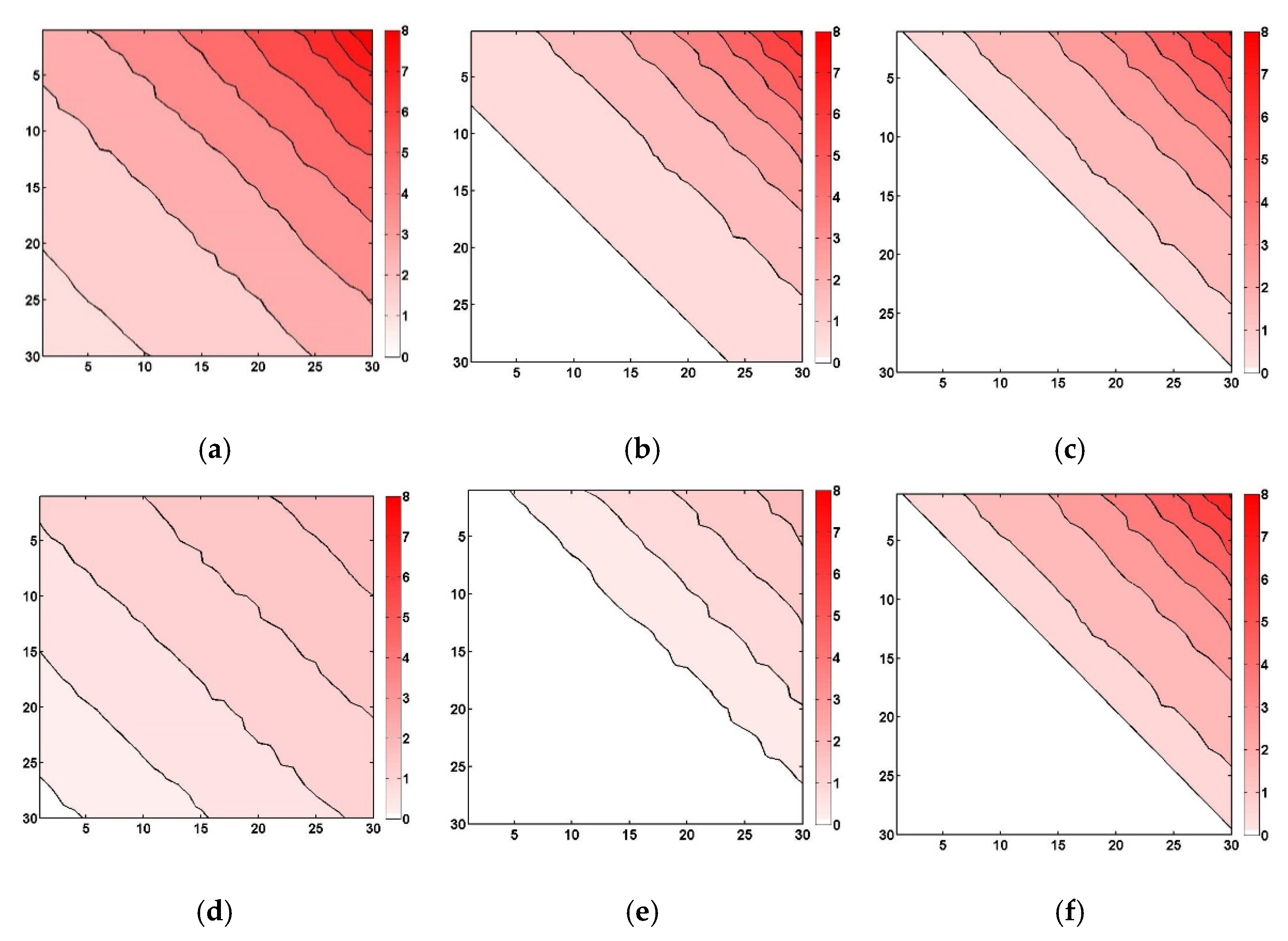
In this part of the study, the effects of data intermittency and data log-normality on the shape of variograms and the application results of simple Kriging were analyzed using synthetic data, as shown in Figure 1. The synthetic data are a kind of imaginary data different from real rain rate data. Among many interesting and complex characteristics of rain rate data, the synthetic data were prepared to show just two characteristics, i.e., data intermittency and log-normality. The synthetic data were generated as follows. First, the synthetic data were assumed to have the structure of 30 × 30 (a total of 900 data points). Second, real (not integer) values from 0 to 8 were assigned from the lower left to the upper right, with a relatively small portion of higher values (Figure 1a; Data 1). Given that similar values were to be located along the diagonal direction, the data structure shows a pattern of diagonal stripe. Third, in order to analyze the effect of data intermittency, two more data fields were made by adding ‘0’ values (Figure 1b,c; Data 2 and Data 3, respectively). The portions of ‘0’ values are 30.7% and 51.7%, respectively. As can be seen in these figures, ‘0’ values are mostly located on the left side of the data. In fact, this was to provide data intermittency in an extreme manner.

Additionally, to analyze the effect of data log-normality, a natural logarithm was applied to these three data (Figure 1a–c). In this case, the ‘0’ values in the original data field were to remain as ‘0’ values in the log-transformed data field. Additionally, the values less than one were assumed to be zero after taking the natural logarithm. This was to prevent negative values, as in rain rate data. This assumption, as a result, increased the portion of zeros, as can be seen in Figure 1d–f.

Means, variances, and maximum values of these six data fields are summarized in

Table 1. Means, variances, and maximum values of three synthetic data.

Data		Mean	Variance	Maximum
Data 1 (‘0’ 0%)	Raw	3.28	2.03	8.00
	Log	1.10	0.18	2.08
Data 2 (‘0’ 30.7%)	Raw	1.38	1.91	7.61
	Log	0.38	0.24	2.03
Data 3 (‘0’ 51.7%)	Raw	1.13	2.24	7.61
	Log	0.35	0.25	2.03

. As can be expected (and as can be found in Table 1), the mean becomes smaller as the portion of zero values increases. This is the same for the log-transformed data. Here, it should be mentioned that the linear trend of the normally distributed data (Figure 1d–f) and the non-linear trend of the log-normally distributed data (Figure 1a–c) were intentionally given to evaluate the application results of Kriging. Thus, in this study, the linear and non-linear trends of the synthetic data were not removed in the following Kriging application.

3.2. Variograms of Synthetic Data

In this study, to evaluate the effect of the data characteristics on the derivation of variograms, four different assumptions with regard to data handling were considered: first, without considering data intermittency and log-normality (Case 1); second, considering only data intermittency (Case 2); third, considering only data log-normality (Case 3); and, finally, considering both data intermittency and log-normality (Case 4). Case 1 was the one in which the data were assumed to be normally distributed and non-intermittent. The variogram in this case was derived by analyzing only the non-zero data without any data transformation to make it follow a Gaussian distribution. The variogram for the log-normally distributed and intermittent data was the complete opposite. Both the zero and non-zero data were considered, and the non-zero data were also transformed to follow a Gaussian distribution. The log-transform was used in this study.

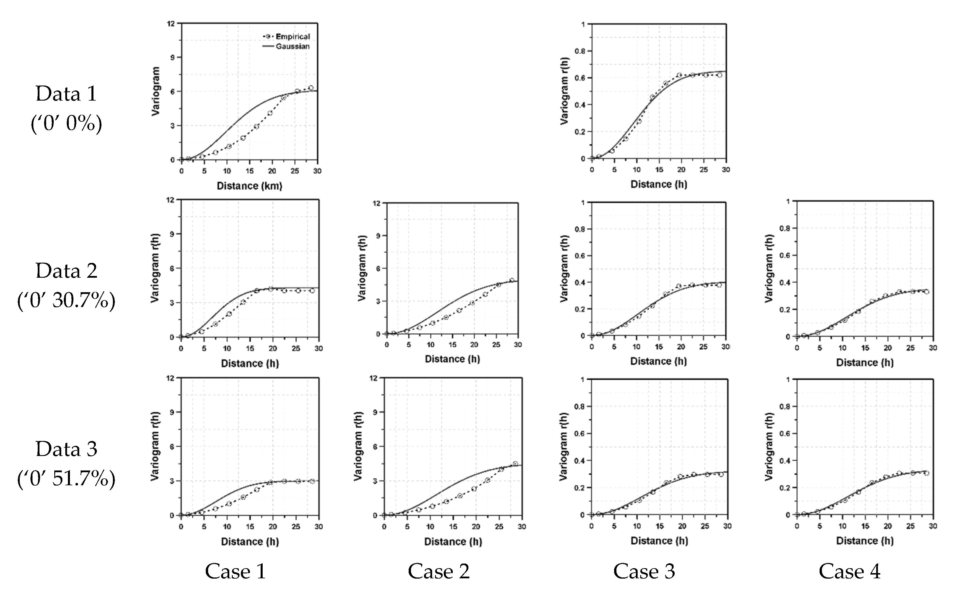
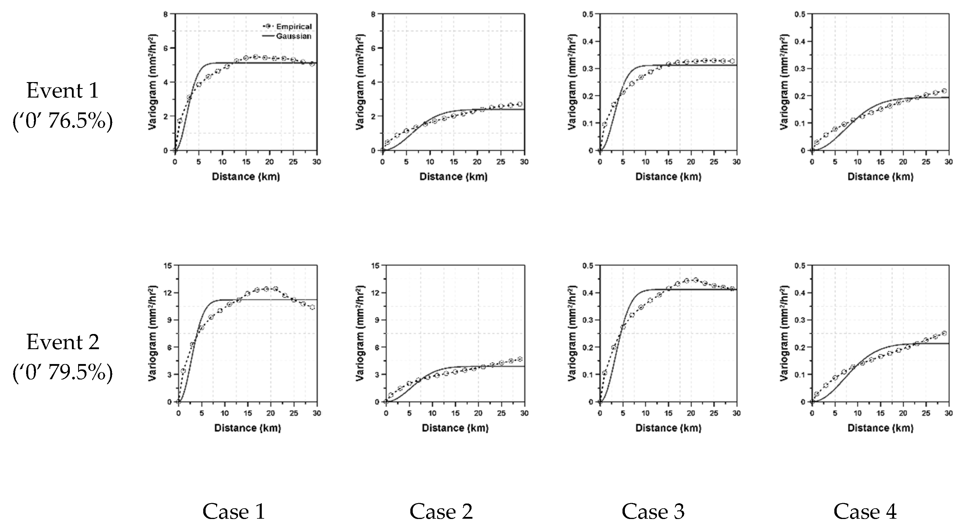
For a theoretical variogram, the Gaussian model was considered. The Gaussian model is known to be suitable for continuous and normally distributed data. However, in this study, the Gaussian model was also applied to the intermittent and log-normally distributed data. In fact, this application was intentional to highlight the problem handled in this study. The least squares method was applied to fit the theoretical variogram. As a result, when the data do not follow a Gaussian distribution, the shape of the empirical variogram should show some mismatch to the Gaussian model. This mismatch can be found in Figure 2, where four different variograms are compared with the Gaussian model.

The dotted line in Figure 2 represents the empirical variogram and the solid line the derived theoretical variogram derived by the Gaussian model. Additionally, in this figure, as Data 1 is that in which intermittency was not considered, only two cases were examined, that is, with and without considering data log-normality. On the other hand, in Data 2 and Data 3, both data intermittency and log-normality were considered in the derivation of variograms. As can be expected, for the cases when only data intermittency was considered (without considering data log-normality), the Gaussian model was found not to fit the empirical variogram properly. This is obvious, as the data do not follow a Gaussian distribution. The empirical variogram shows the pattern of accumulated exponential function, different from the S-curve of the Gaussian model. On the other hand, when considering data log-normality along with data intermittency, the Gaussian model was found to fit the empirical variogram well. This result proved the importance of considering data characteristics when deriving variograms. The sill heights and correlation lengths derived by fitting the Gaussian model to the empirical variograms are summarized in

Table 2. Sill heights and correlation lengths of variograms estimated for the synthetic data.

Synthetic Data		Sill Height	Correlation Length
Data 1 (‘0’ 0%)	Case 1—without considering data intermittency and log-normality	6.1	23.7
	Case 2—considering only data intermittency	-	-
	Case 3—considering only data log-normality	0.7	22.3
	Case 4—considering both data intermittency and log-normality	-	-
Data 2 (‘0’ 30.7%)	Case 1	4.3	16.5
	Case 2	4.9	27.6
	Case 3	0.4	25.1
	Case 4	0.4	26.3
Data 3 (‘0’ 51.7%)	Case 1	3.0	18.5
	Case 2	4.5	27.8
	Case 3	0.3	26.3
	Case 4	0.3	27.1

.

As can be seen in Table 2, the correlation length derived by considering both data intermittency and data log-normality was longer than those correlation lengths that were not so derived. Even the correlation lengths derived by considering only data intermittency or data log-normality were also found to be longer than those derivations that considered neither. Among the two, data log-normality was found to have a stronger effect on correlation length than data intermittency. However, the longer correlation length estimated when considering only data intermittency seemed to be partly affected by the improperly fitted variogram. As the Gaussian model could not properly fit the data in the case of considering only data intermittency, the correlation length happened to be estimated as being much longer.

The sill height seemed not to be affected by data log-normality in this application with the synthetic data. Any obvious tendency could not be found. However, the effect of data intermittency on the sill height was rather clear. That is, the sill height was estimated to be smaller with more zero values.

3.3. Kriging Results

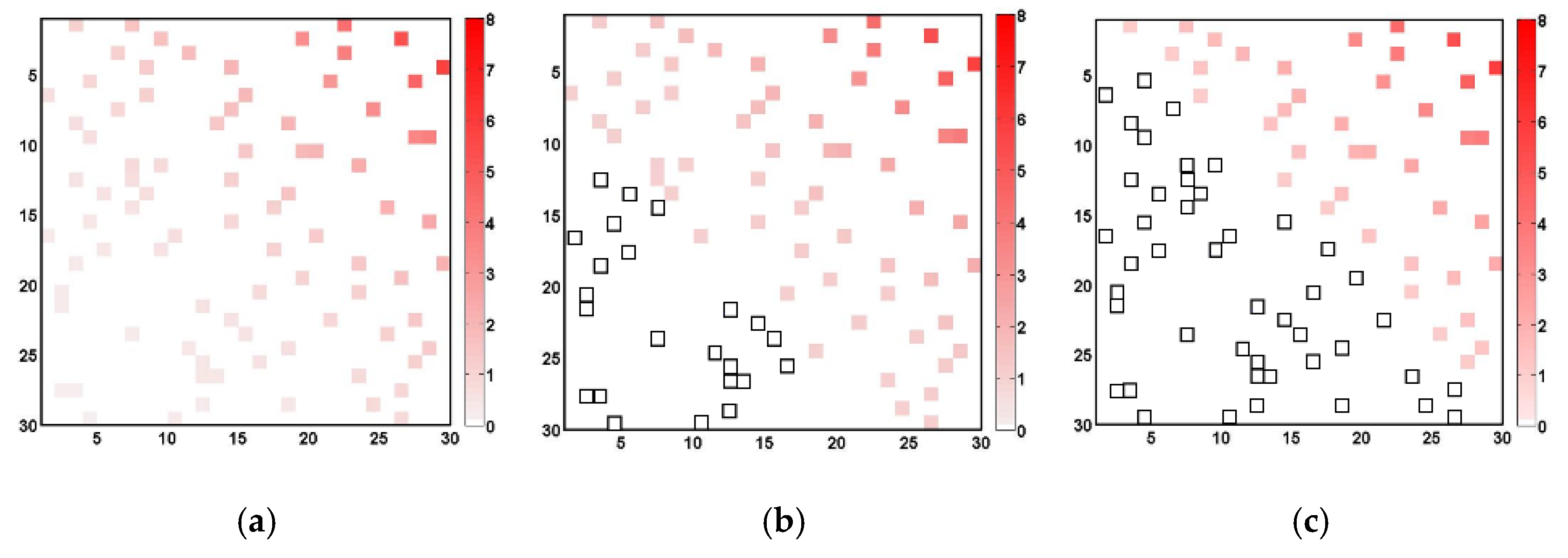
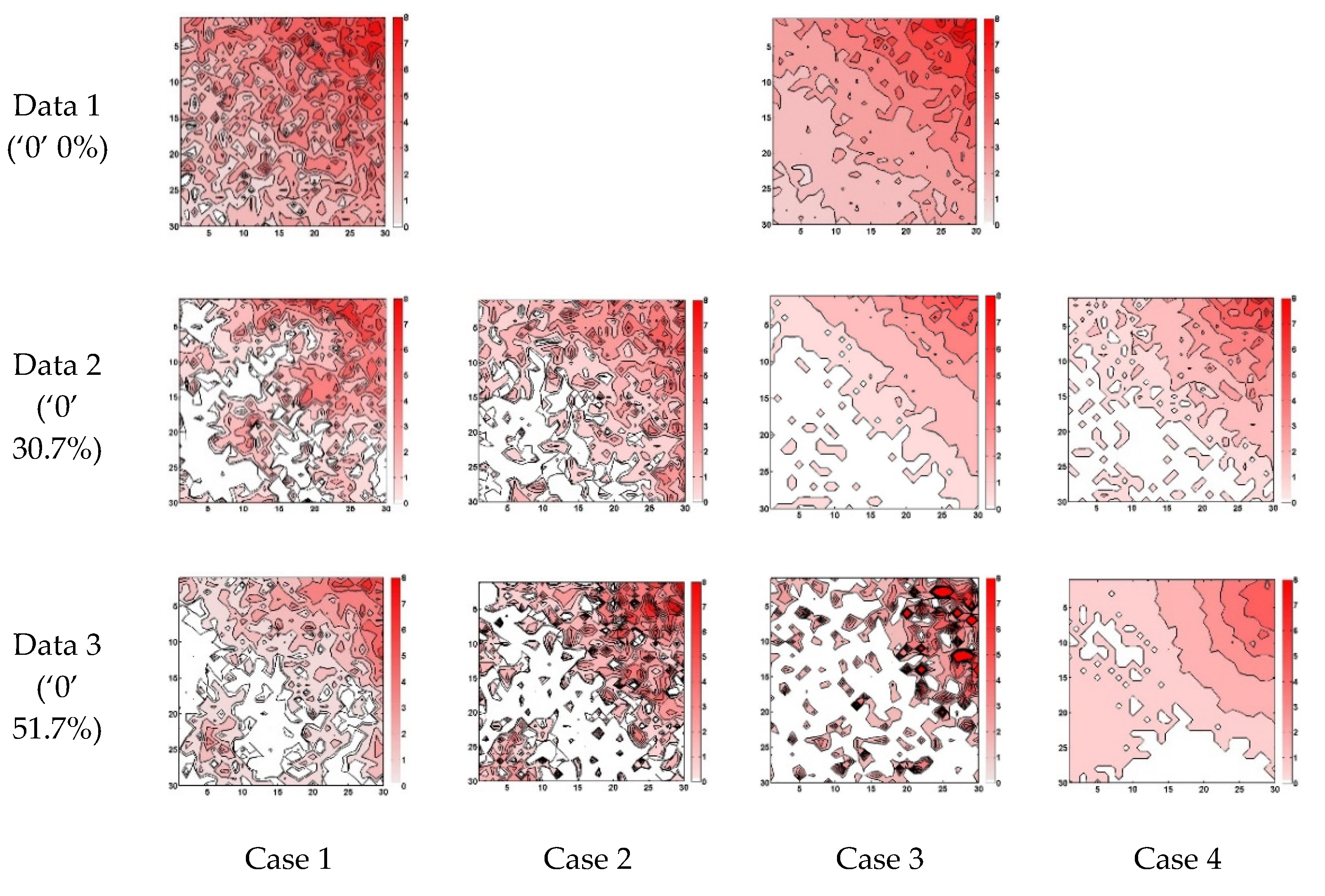
To evaluate the application results of simple Kriging, a total of 90 data points (about 10% out of the entire data field) were selected randomly from the synthetic data presented in Figure 1; these are presented in Figure 3. This random selection was made to mimic a real sparse rain gauge network. Simple Kriging was then applied to generate the data field with the variograms determined as in Figure 2, derived by considering data intermittency and/or data log-normality. When applying simple Kriging to the case of considering data log-normality, the original data were transformed to follow a Gaussian distribution by taking the natural logarithms. The application results of simple Kriging to four different cases considered in this study are presented in Figure 4.

When considering only data intermittency, the Kriging result was closer to the original data than that obtained without considering data intermittency. However, in this case, it was also found that several abnormally high values were generated to make the contour lines very complex. This is mainly due to the effect of the long correlation length. Furthermore, most of the zero values in the original data disappeared due to the longer correlation length.

Similar to the case considering data intermittency, consideration of the data log-normality was also found to generate a data field closer to the original data. The same problem of generating non-zero measurements was also found. However, this negative effect was relatively small, making the generated data field much closer to the original data. It should also be noted that, in Data 3, some extreme values were generated to make the contour lines slightly different from the original data.

When considering both the data intermittency and data log-normality, it was found that many more zero values were replaced by positive values than those in the previous two cases. However, especially in Data 3, the abnormally high values were not generated, and, as a result, the generated data field became more similar to the original data. A summary of these results by the mean, maximum value, RMSE (root mean square error), and BS (bias) is given in

Table 3. Means, maximum values, RMSEs, and BSs of simple Kriging results for the synthetic data.

	Case 1—Without Considering Data Intermittency and Log-Normality				Case 2—Considering Only Data Intermittency				Case 3—Considering Only Data Log-Normality				Case 4—Considering Both Data Intermittencyand Log-Normality
	Mean	Max.	RMSE	BS	Mean	Max.	RMSE	BS	Mean	Max.	RMSE	BS	Mean	Max.	RMSE	BS
Data 1 (‘0’ 0%)	3.26	8.57	1.138	0.995	-	-	-	-	3.37	10.28	0.467	1.027	-	-	-	-
Data 2 (‘0’ 30.7%)	1.38	8.86	1.634	1.004	1.30	7.07	1.368	0.944	1.28	6.43	0.536	0.926	1.38	8.50	0.647	1.006
Data 3 (‘0’ 51.7%)	1.03	7.36	1.209	0.905	0.87	11.56	2.245	0.768	1.82	27.16	2.521	1.601	1.42	5.25	0.745	1.250

. Here, RMSE is an index that evaluates the differences between the Kriging results and the original synthetic data, and BS represents a comparison of the mean ratios.

As can be found in Table 3, means and maximum values for Data 1 and Data 2 are similar to those of the original data. However, in Data 3, the mean and maximum values were rather high than the original data. For example, for Data 3, when considering only data log-normality, the maximum value generated was 27.16, about 3.5 times higher than just 7.61 in the origin data. The mean of the synthetic data was also 61% higher than the original data—increased from 1.13 to 1.82. As mentioned earlier, this result was due to the longer correlation length.

In both Data 1 and Data 2, the RMSE derived considering both data intermittency and data log-normality with simple Kriging was found to be smaller than that derived without considering these data characteristics. In Data 1, the RMSE was estimated to be 1.138 under the assumption of data normality. However, when considering data log-normality, the RMSE was much smaller—0.467, about 59% smaller than the original value. This result was the same in Data 2, when the RMSE was estimated to be 1.634, but was 1.368 (16.3% smaller) when considering data intermittency and 0.536 (67.2% smaller) when considering data log-normality. When considering both data intermittency and data log-normality, the RMSE became 0.647 (60.4% smaller). In Data 3, the RMSE was estimated to be 1.209 without considering the data characteristics and was 0.745 (38.3% smaller) when considering both data intermittency and data log-normality. Interestingly, also different from Data 2, the RMSE when considering only data intermittency was estimated to be higher—2.245 (86.2% higher)—and when considering only the data log-normality it was 2.521 (108.6% higher). This problem in Data 3 was mainly due to the abnormally high correlation length estimated when considering either data intermittency or data log-normality.

The BSs in Data 1 and Data 2 were all found to be near 1. In fact, this result is not so surprising given that the Kriging result should have a similar mean to the original data. However, in Data 3, when only data intermittency was considered, the BS was estimated to be just 0.768. That is, the mean of the Kriging result was smaller than that of the original data. On the other hand, when only considering data log-normality, the BS was estimated to be 1.601, that is, a high mean value for the Kriging result. This result can also be confirmed by abnormally high values generated for the Kriging result, as in Figure 4. On the other hand, when considering both data intermittency and data log-normality, the BS was calculated to be 1.250. The serious underestimation and overestimation problem when considering only data intermittency or data log-normality was somewhat alleviated.

4. Discussion of the Possible Application to Rain Rate Data

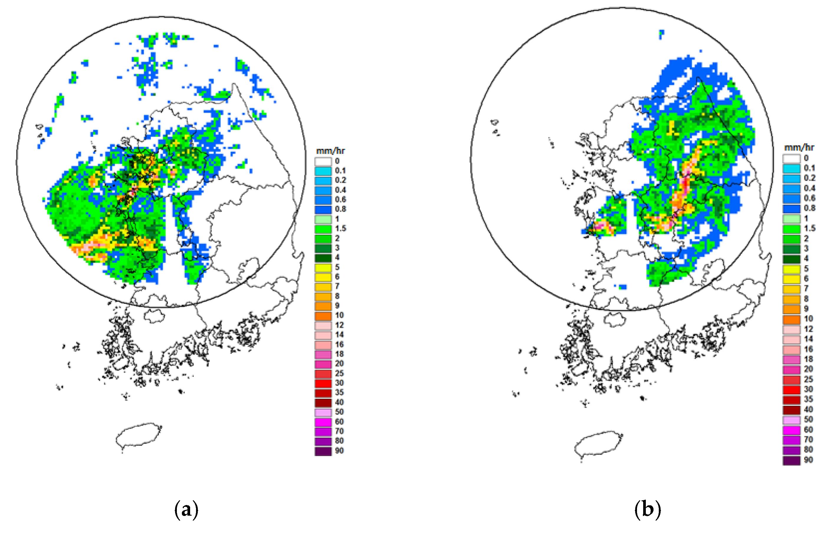
Rain rate data are generally assumed to be typical log-normal and intermittent data. If this assumption is true, the above consideration of data intermittency and log-normality in the previous section should also be valid for rain rate data. To evaluate this hypothesis, this study used the rain rate data observed at 45 rain gauge stations within the umbrella of the Gwanaksan radar in Korea, and simple Kriging was applied to make the rain rate field. Among available data sets, this study selected two data sets for further application: one was the rain rate field observed at 4:30 on 11 September 2010 (Event 1) and the other was at 8:30 on the same day (Event 2). The portion of no rain in these rain rate fields was 76.5% for Event 1 and 79.5% for Event 2. The radar images for these two rain rate fields are given in Figure 5. The variograms were determined as in Figure 6.

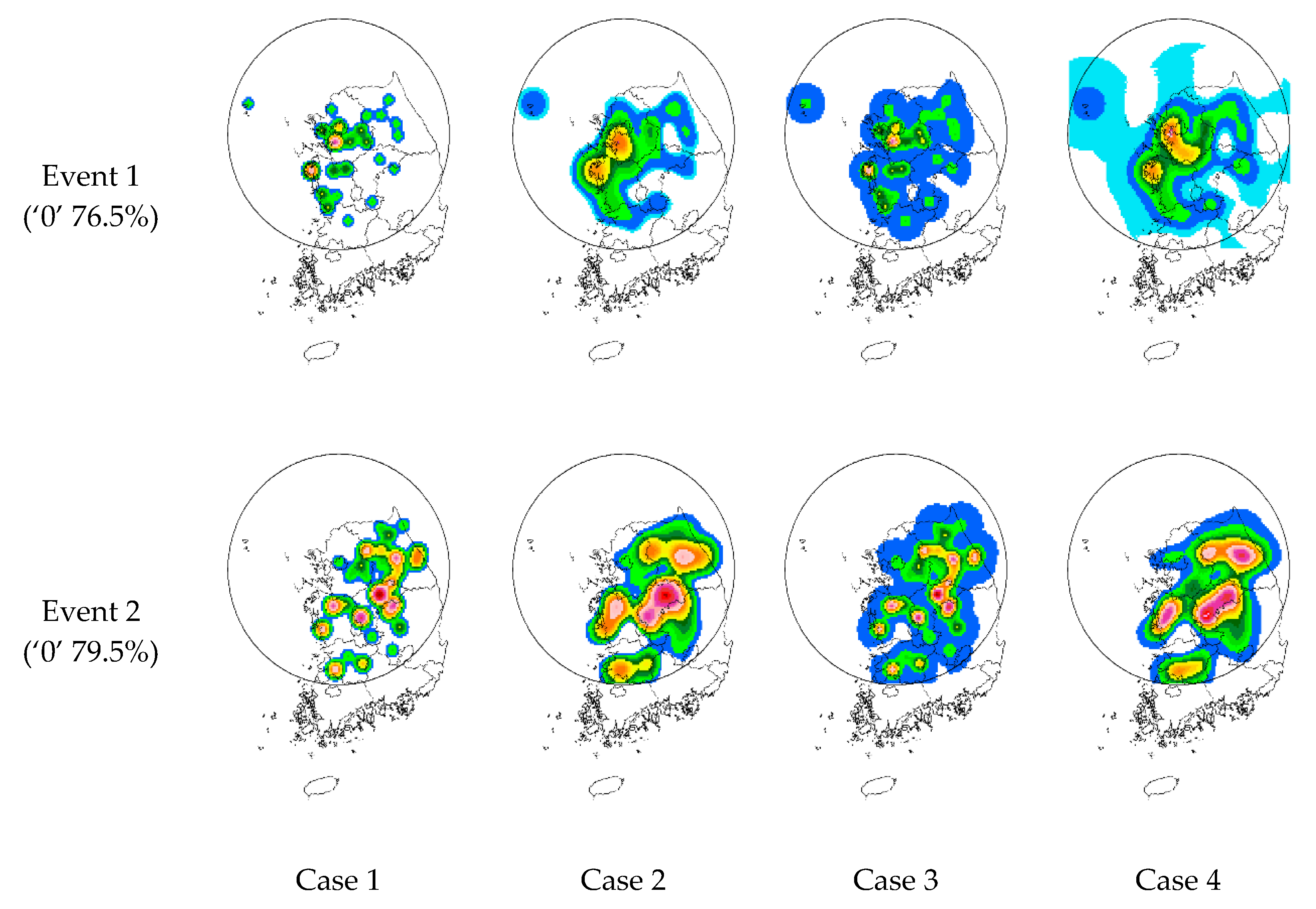
A total of four different cases, similar to the synthetic data analysis, were considered to make the rain rate field. First, the original data were applied to the simple Kriging with and without considering data intermittency. In these two cases, the data log-normality was not considered. Second, the original data were transformed by taking the natural logarithm to follow a Gaussian distribution. The transformed data were then applied to the simple Kriging with and without considering data intermittency. The Kriging results were then inverse-transformed to be compared with the original radar rain rate field. A total of four different rain rate fields generated by the simple Kriging with different considerations of data intermittency and/or data log-normality are compared in Figure 7. It should be noted that the anisotropy was not considered in the generation of rain rate fields. For this reason, the generated rain rate fields show a somewhat circular pattern compared to the radar rain rate field.

The generated rain rate fields can be compared from several aspects. First, the rain rate field generated without considering either data intermittency or data log-normality shows the smallest rainfall spatial coverage. This is simply because the correlation length in this case is the shortest. However, due to the relatively high sill height, some high rain rate data could be generated. Second, consideration of data intermittency has a tendency to increase correlation length. Thus, the rain rate field generated shows much larger rainfall spatial coverage than the previous case. On the other hand, as the sill height was estimated to be smaller than that in the previous case, rather high rain rate values could not be generated. Consideration of data log-normality resulted in a somewhat larger rainfall spatial coverage than in the case considering data intermittency. Furthermore, in this case, rather high rain rate data were generated. Third, in the case of considering both data intermittency and data log-normality, the rainfall spatial coverage was found to be the largest. This result was very much expectable, as the correlation length in this case was the longest. Additionally, it should be noted that high rain rate data were also generated in this case. Another problem in this case was that the low rain rate values were generated where zero measurements had been observed in the original data.

The mean rain rates and maximum rain rates of the four rain rate fields generated are compared in

Table 4. Same as Figure 3, but for rain rate data.

	Case 1—without Considering Data Intermittency and Log-Normality				Case 2—Considering Only Data Intermittency				Case 3—Considering Only Data Log-Normality				Case 4—Considering Both Data Intermittency and Log-Normality
	Mean	Max.	RMSE	BS	Mean	Max.	RMSE	BS	Mean	Max.	RMSE	BS	Mean	Max.	RMSE	BS
Event 1	0.29	21.01	1.965	0.363	0.63	21.00	1.825	0.783	0.55	20.74	1.869	0.687	0.89	23.25	1.883	1.110
Event 2	0.61	42.00	3.620	0.753	1.11	42.23	3.413	1.370	0.64	41.05	3.492	0.791	1.09	52.66	3.501	1.342

. In addition, the BSs and RMSEs estimated with respect to the radar rain rate are provided in the same table. The mean rain rates of the cases without consideration of data intermittency were found to be 21% to 64% smaller than the observed radar rain rate. On the other hand, the mean rain rates generated by considering data intermittency were mostly higher than the radar rain rate. In the case of considering both data intermittency and data log-normality, the mean rain rates were estimated to be 11.3% higher for Event 1 and 34.6% for Event 2.

The maximum rain rates of the first three cases (with or without consideration of data intermittency or data log-normality) were found to be slightly smaller, by 5% to 6%, than the observed radar rain rate for Event 1. In the case of considering both data intermittency and data log-normality, the maximum rain rate increased by 5% above the radar rain rate. On the other hand, for Event 2, the maximum value was 18% to 50% larger than the radar rain rate data in all cases. These results show that the portion of the high rain rate region in the original data field for Event 2 was larger than that for Event 1. As can also be seen in Figure 7, it can be concluded that simple Kriging generated a very smooth data field.

The estimated BSs are more or less the same as the ratios of mean rain rates to the radar rain rate. In the case that did not consider data intermittency, the BS estimated was 0.4 to 0.8 for both Event 1 and Event 2. However, the BSs were mostly higher than 1.0 when considering data intermittency. In the case of considering both data intermittency and log-normality, BSs were higher than one—1.11 for Event 1 and 1.34 for Event 2. These results are similar to the previous comparison of the mean rain rates.

Interestingly, the RMSE was estimated to be smallest for the case considering only data intermittency. The RMSE was estimated to be 1.97 for Event 1 when considering neither data intermittency nor data log-normality, but it was 1.83 (7.1% smaller) when considering only data intermittency, 1.87 (4.9% smaller) when considering only data log-normality, and 1.88 (4.2% smaller) when considering both data intermittency and data log-normality. For Event 2, the RMSEs were estimated to be 3.62, 3.41 (5.7% smaller), 3.49 (3.5% smaller), and 3.50 (3.3% smaller), respectively. These result were mostly for an area with no rain. Especially in the case considering only data intermittency, most of the area with no rain was found to be the area with zero measurements, which can be seen in Figure 7. When considering data log-normality, the area with no rain has decreased considerably.

Overall, it is true that consideration of data intermittency and data log-normality can improve simple Kriging results. The effect of considering data intermittency was found to be very significant. However, the effect of considering data log-normality could still not be confirmed. This result indicates that rain rate data do not fully follow the log-normal distribution. The positive estimation of rain rate over the area with no rain seems to be the most serious problem.

5. Summary and Conclusions

This study evaluated the effect of data intermittency and log-normality on the application of simple Kriging. First, a synthetic data, both intermittent and log-normal, was prepared for this purpose, then four different Kriging applications were repeated with this synthetic data under different assumptions of data intermittency and log-normality. The effects of those assumptions on the simple Kriging applications were evaluated and compared with each other. The possible application of the derived results to rain rate data was also discussed in relation to the observed rain gauge data within the Gwanaksan radar umbrella in Korea.

First, the effect of data intermittency and log-normality on the shape of variograms was found to be significant. Basically, the correlation length derived for a variogram was longer when considering both data intermittency and data log-normality. Furthermore, the sill height of the variogram was estimated to be smaller, especially when data intermittency was high. Overall, the effect of data log-normality on variograms was found to be greater than that of data intermittency.

Several evaluation measures, such as mean, maximum value, RMSE and BS, indicated that the fields generated by simple Kriging were much closer to the original data when considering data intermittency and log-normality. However, several abnormally high values were noticed and the portion of zero values was also found to be smaller than the original data. When considering both data intermittency and data log-normality, many more zero values were replaced by positive values, but abnormally high values were much fewer than in the previous cases. As a result, the data field generated by considering both data intermittency and data log-normality became more similar to the original data.

Similar results could also be derived in the application to the rain rate data observed by rain gauges within the Gwanaksan radar umbrella. The effect of considering data intermittency was especially clear. However, the effect of data log-normality was somewhat arguable. Consideration of data log-normality did not significantly improve the results for the simple Kriging application. This may be due to the fact that the rain rate data did not fully follow a log-normal distribution.

Based on the findings in this study, it was confirmed that the consideration of data characteristics could improve the quality of simple Kriging applications. However, sometimes, it may not be a simple problem to consider data characteristics. There can be cases where no specific data characteristics are known. It is also possible that a unique probability distribution function cannot fully describe the observed data. In this study, it was found that the assumption of log-normality was not so effective in the application to the observed rain rate data. These problems should be solved by applying an appropriate data distribution function. Further studies are required to solve this problem. Additionally, deriving any obvious patterns, trends, and anisotropy in rainfall data in space is another problem. Further study should focus on these issues and the insights they provide may contribute to the solution of more complicated problems, such as the merging of non-normal intermittent bivariate data.