Article

Differences in Spatiotemporal Variability of Potential and Reference Crop Evapotranspirations

1
College of Water Resources and Architectural Engineering, Shihezi University, Shihezi 832003, China
2
College of Water Resources and Architectural Engineering, Northwest Agriculture and Forestry University, Xianyang 712100, China
3
Institute of Agricultural Science of the Third Division of Xinjiang Production and Construction Corps, Tumushuke 843900, China
4
Key Laboratory for Agricultural Soil and Water Engineering in Arid Area of Ministry of Education, Northwest A&F University, Xianyang 712100, China
5
School of Environmental Sciences, University of Guelph, Guelph, ON N1G 2W1, Canada
6
NSW Department of Primary Industries, Wagga Wagga Agricultural Institute, Wagga Wagga, NSW 2650, Australia
7
Tashkent Institute of Irrigation and Agricultural Mechanization Engineers—National Research University, Qoriy Niyoziy 39, Tashkent 100000, Uzbekistan
8
Academy of Plateau Science and Sustainability, Qinghai Normal University, Xining 810008, China
*
Authors to whom correspondence should be addressed.
These authors contributed equally to this work.
Water 2022, 14(6), 988; https://doi.org/10.3390/w14060988
Submission received: 9 February 2022 / Revised: 15 March 2022 / Accepted: 17 March 2022 / Published: 21 March 2022
(This article belongs to the Section Hydrology)

Abstract

:
Potential evapotranspiration (ETp) and reference crop evapotranspiration (ETo) are two key parameters in hydrology, meteorology, and agronomy. ETp and ETo are related to each other but have different meanings and applications. In this study, the ETp and ETo were distinguished and calculated with the Penman and FAO56 PM equations using the weather data of 551 stations in China from 1961 to 2018. The differences in their spatiotemporal variations were examined with an MMK test, an R/S test, and wavelet analysis. The monthly ETp and ETo were close but the ETp was always larger than the ETo, with values ranging from 1 to 356 mm and 2 to 323 mm, respectively. Their differences varied in different months and sub-regions. The maximum monthly difference transferred from south to north and then back to the south in a yearly cycle, showing spatiotemporal heterogeneity. The annual values of the ETp and ETo were also close, but the ETp was significantly higher than the ETo. The increasing future trends of ETp but decreasing trends of ETo were tested at most sites in China. Although the primary periods were almost the same, their spatial distribution was slightly different. In conclusion, ETp is different from ETo and they should be applied carefully. This study performs a thorough comparison and reveals the underlying basis of and discrepancy between ETp and ETo.

1. Introduction

Potential evapotranspiration (ETp) and reference crop evapotranspiration (ETo) are closely connected to actual evapotranspiration (ET) [1,2], leading them to be extensively used in the fields of hydrology, agronomy, meteorology, and ecology [1,2,3,4,5]. Moreover, an important practical application of ET in the fields mentioned above is crop evapotranspiration (ETc) [6], which is usually calculated by ETp or ETo to evaluate the regional or global variation in agricultural water quantity [7,8], to assess the impacts or responses to climate change [9,10,11], and to provide useful guidelines for related policy makers. The accuracy estimation of ETp or ETo is key for achieving these aims. Therefore, the difference between ETp and ETo needs further analysis. Many recent research involving ETp or ETo has focused on their variation, regional characteristics [12] or prediction [13], drought or drying analysis [14], vegetation responses [15], responses to drought [16], the influence of water resources on agriculture [17], and evapotranspiration rate estimations [18]. The studied timescales varied from monthly to annual [2,19], and the spatial scales varied from site [20] to multi-site [19], regional [21], national, and global. Additionally, many interesting results were obtained, the calculation efficiency was improved, and a software was created [22].
The development of definitions for ETp and ETo has been a long-term process. Thornthwaite (1948) defined ETp as “the maximal water vapor in an area, including the evapotranspiration from crops and the evaporation from water surfaces in order to determine dry/wet conditions” [23]. Although other definitions have been suggested [24,25,26,27,28,29], the definition of ETp has not yet been standardized. Doorenbos and Pruitt (1977) proposed a clear concept of ETo [30]. The Food and Agriculture Organization (FAO) standardized the ETo definition as “the ratio of evapotranspiration from a reference crop with an assumed crop height of 12 cm, a fixed surface resistance at 70 s/m, and albedo of 0.23 which closely resembles evapotranspiration from an extensive surface of green grass cover without water stress” [6].
Despite some similarities, there are many differences between ETp and ETo in terms of their definition, estimation methods, equation types, and application fields. Much of the previous research has mixed the utilization of these two terms. Instances of this misuse are as follows. (i) Use of incorrect terminology [31,32,33]: For example, Sun et al. adopted the FAO 56 Penman–Monteith equation to estimate ETo, but they named it “potential evapotranspiration” [34,35]. (ii) The alternative and inconsistent use of the two terms (Gwate et al., 2018; Lewis and Allen 2017; Zhang 2019) [5,36,37]: When Ding et al. (2020) adopted the FAO 56 Penman–Monteith equation to estimate ETo in northwest China, they used both terms—“potential evapotranspiration” and “reference evapotranspiration” [38]. (iii) The application of mixed equations. For example, Oudin et al. (2005) generalized four different types of ETp, when in fact the FAO-24 and Hargreaves and Samani (1982) were ETo equations. Burke et al. (2006) adopted an ETo equation to estimate ETp when conducting a drought analysis [30,39,40,41,42].
Except for some common misuses, most researchers have used ETo [6,43,44,45,46,47,48,49] or ETp correctly [50,51,52]. However, their attributions have rarely been compared. For example, Katerji and Rana (2011) investigated the differences between ETp and ETo by comparing resistances (namely, the aerodynamic resistance, crop-structure resistance and crop-stomatal resistance) [53]. They concluded that ETo and ETp were un-equivalent. Xiang et al. (2020) reviewed the differences between the two terms and grouped the different types of ETp and ET0 [54]. This was the first study to clearly differentiate ETp and ETo up until now.
Many researchers consider ETp and ETo to be equivalent. Due to the difficulty in their direct and accurate measurement, the differences in these closely related terms when supporting and modelling results are often considered to be errors or uncertainties, even though these can be reduced through the proper choice of the type of ET. Accuracy estimations of ETp and ETo affect both the water-resource and agricultural sectors and contributes significantly to the national economy [50]. Although there has been progress in differentiating ETp and ETo, a direct quantitative comparison between them is missing, despite their contributions to the fields of agriculture, engineering, and the environment. Thus, this research aims to quantitatively compare ETp and ETo at monthly and annual timescales for mainland China based on their commonly used and standardized methods. The spatiotemporal variability characteristics, including trends, abrupt-change years, the wavelet-based main- and quasi-periods, and the serial long-term dependence, will be systematically compared. This work will provide important references for researchers in a wide range of fields who directly or indirectly use potential or reference crop evapotranspiration.

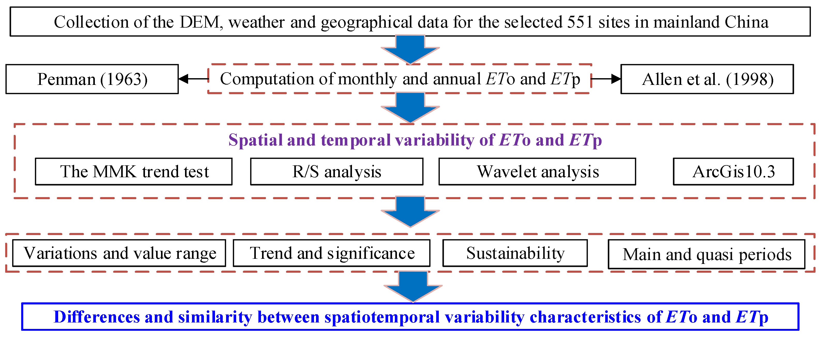
2. Data Collection and Methodology

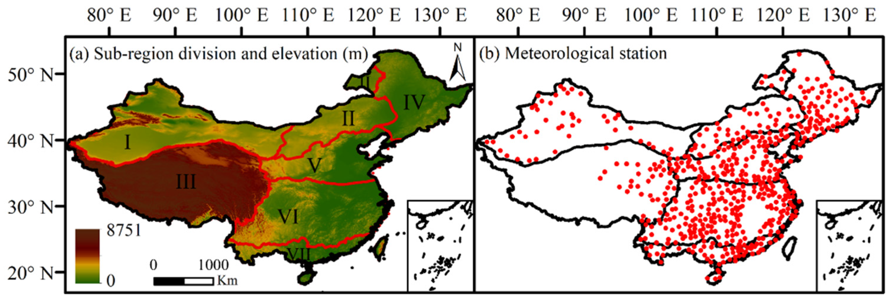
2.1. Study Area Description and Data Sources

China is located in eastern Eurasia on the west coast of the Pacific Ocean. It has a large land mass (9.634057 × 10⁶ km2); a long distance between its eastern and western boundaries; a wide range of altitudes, morphologies, and mountains; and a variety of climates. Weather data from 839 stations of China were downloaded from the Meteorological Data Sharing Service Network in China (http://data.cma.cn/, accessed on 6 March 2017). The daily climatic variables include precipitation, wind speed at 10 m (u10), the maximum (Tmax) and minimum air temperature (Tmin), relative humidity, and hours of sunshine, from December 1960 to December 2018. The sites with a data-missing ratio >1% were removed. Missing data were interpolated with the data of 10 adjacent sites on the same day. The data were cross-examined using the Kendall autocorrelation and Mann–Whitney homogeneity tests [55]. The test results indicated that the fluctuation of the weather data was fixed between critical points at a significance level of 5% [56,57]. Finally, a total of 551 sites were selected.
The digital elevation and the site distribution in mainland China are presented in Figure 1. There are seven climate zones, including the northwestern desert region, the Inner Mongolia grassland region, the Qinghai–Tibetan Plateau, the northeastern humid and sub-humid region, the northern China humid and semi-humid region, the middle and southern China humid and sub-tropical region, and the southern China humid and tropical region, which are named as sub-regions I to VII and which contain 46, 47, 39, 69, 108, 190, and 52 weather stations, respectively. Sub-region III contains fewer stations due to its relatively rough terrain with high elevation range. The analysis will consider both mainland China and these divided sub-regions.

2.2. Methodology

2.2.1. Equations for Estimating ETp and ETo

The Penman (1963) equation was selected as the standaridized ETp method, since this formula was developed from the Penman (1948) equation and is one of the earliest methods used to calculate ETp [25]. It is a widely used equation [58,59,60], written as [25]:
E T p = Δ Δ + γ ( R n G ) + 6.43 γ Δ + γ ( 1 + 0.0536 u 2 ) ( e s e a )
where Δ is the slope of the vapor–pressure curve (kPa °C−1); γ is the psychrometric constant (kPa °C−1); u2 and T2 are the wind speed (m s−1) and mean air temperature (°C) at 2 m; es and ea are the saturation and actual vapor pressure (kPa), respectively (kPa); Rn is the net radiation (MJ m−2 day−1); and G is the soil heat flux (MJ m−2 day−1). Values of u2 are obtained based on u10. G at the M th month is estimated by the soil temperature of M+1 th and M−1 th month:
GM = 0.07 (TM+1TM−1)
The standaridized ETo method of the Penman–Monteith equation is written as [6]:
E T o = 0.408 Δ ( R n G ) + γ u 2 ( e s e a ) [ 900 / ( T 2 + 273 ) ] Δ + γ ( 1 + 0.34 u 2 )
Annual ETo or ETp values are found by summing the monthly values.

2.2.2. Trend and Abrupt-Change Year Analysis

The trends and significance of the annual ETo (or ETp) series at the 551 sites were tested following the modified nonparametric Mann–Kendall (MMK) method [61]. The MMK considers the effects of self-correlation in time series x(t) (t = 1, 2, …, NT, where NT is the total year number) based on the Mann–Kendall method [62,63]. To show the influence of serial self-correlation, the MK statistic is modified to the new MMK statistic (Zm) with a correction factor ns [64]. If Zm is positive/negative, x(t) has an up/downward trend. When the lag of self-correlation functions is >0 and |Zm| ≥ 1.96, xi is time-dependent and the trend is significant at a confidence level α = 0.05. The equations are written as follows:
Z * = Z n 1 s ,   w h e r e   n 1 s = { 1 + 2 n 1 j j = 1 n 1 1 ( n 1 1 ) r j j                               f o r   j j > 1 1 + 2 r 1 n 1 + 1 n 1 r 1 2 + ( n 1 1 ) r 1 n 1 ( r 1 1 ) 2                   f o r   j j > 1
where rjj is the self-correlation coefficient of the time series at the lag-jj.

2.2.3. The Rescaled (R/S) Analysis

The R/S analysis was proposed based on Hurst (1951) [65,66]. For the time series x (t) (t = 1, 2, ···58), the mean value and cumulative deviation of the sub-series are calculated as:
y ( τ ) = 1 τ t = 1 τ x ( τ ) ,   τ = 1 , 2 ,  
F ( t , τ ) = u = 1 τ x ( u ) y ( τ ) ,   1     t     τ  
The range is calculated as:
R ( τ ) = max 1 t τ F ( t , τ ) min 1 t τ F ( t , τ ) ,   F ( t , τ ) = 1 , 2 ,  
Additionally the standardized deviation is computed as:
S ( τ ) = [ 1 τ t = 1 τ ( x ( t ) y ( τ ) ) 2 ] 1 2   ,   τ = 1 , 2 ,  
The ratio of the range to standardized deviation is described as:
R ( τ ) S ( τ ) = ( C τ ) H   ,   then   log   ( R / S ) n = logc + H log n  
where C is a constant. By applying Equation (11), the Hurst index (0 < H < 1) is obtained. H measures the intensity of long-range dependence in x(t). When H = 0.5, the time series x(t) has a random process. When 0 < H < 0.5 and 0.5 < H < 1, x(t) has reversibility or sustainability, respectively.

2.2.4. The Wavelet Analysis

A continuous wavelet transform was performed using the Morlet wavelet basis ( Ψ 0 ) [67]. The wavelet key function is described as:
+ Ψ ( t ) dt = 0
where t is the year and Ψ(t) is a wavelet function that can form a cluster of functions on the timeline (Li et al., 2019):
Ψ a , b ( t ) = | a | 1 2 Ψ ( t b a ) ,   a , b R , a 0
where Ψa,b(t) is a sub-wavelet, a is a wavelet-length scale factor, and b is a factor that shows the translation in time. The multi-Morlet-wavelet was selected as a basic function here.
The primary period has a maximum vibration intensity showing the significance or insignificance which is read from the bright color-belt of the wavelet map. The quasi-period has a secondary maximum vibration intensity [68]. The MATLAB 2019b software (MathWorks, Natick, MA, USA) was used to perform these analyses.
A schematic of general framework adopted in this research is presented in Figure 2.

3. Results

3.1. The Differences between Monthly ETp and ETo

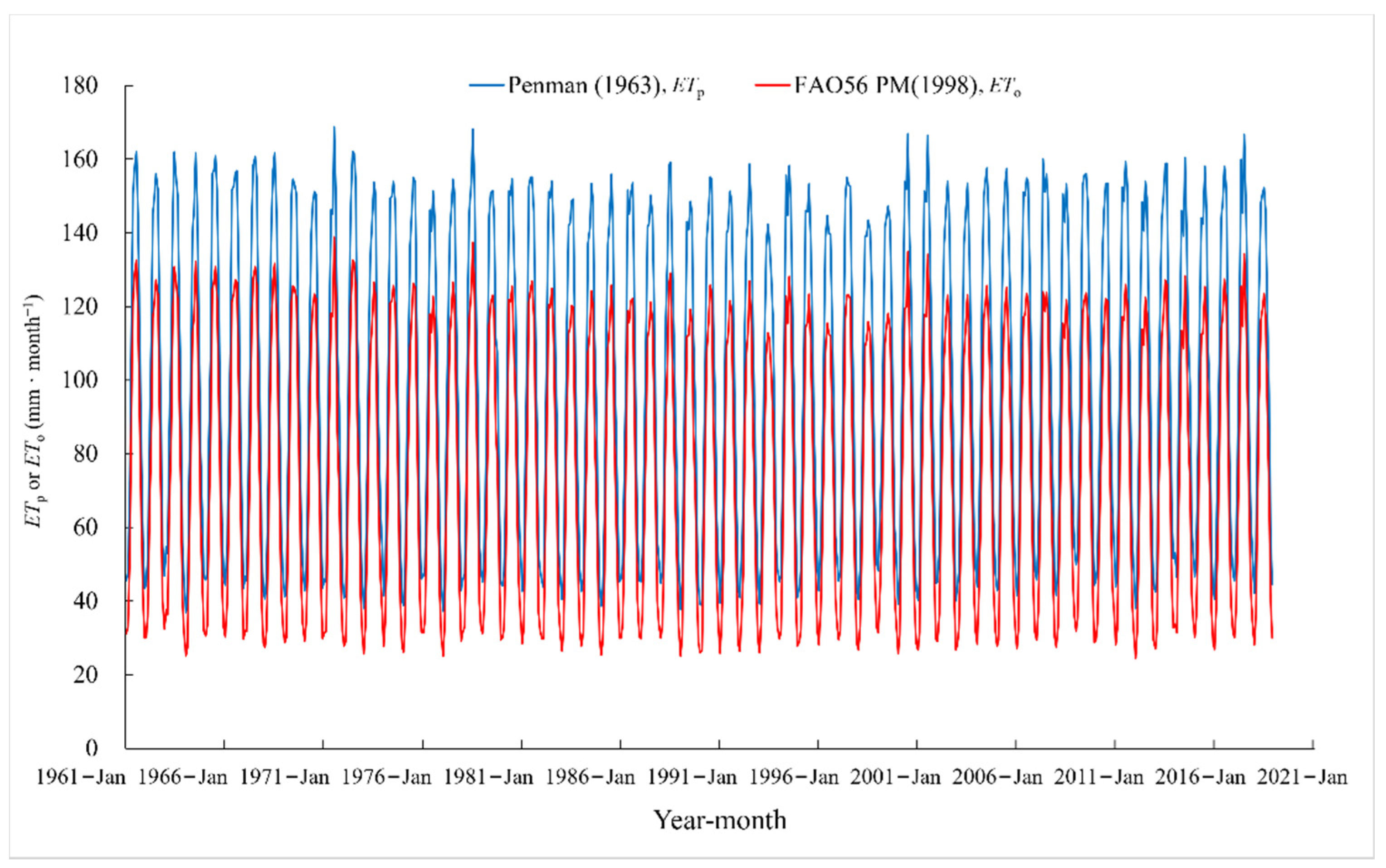
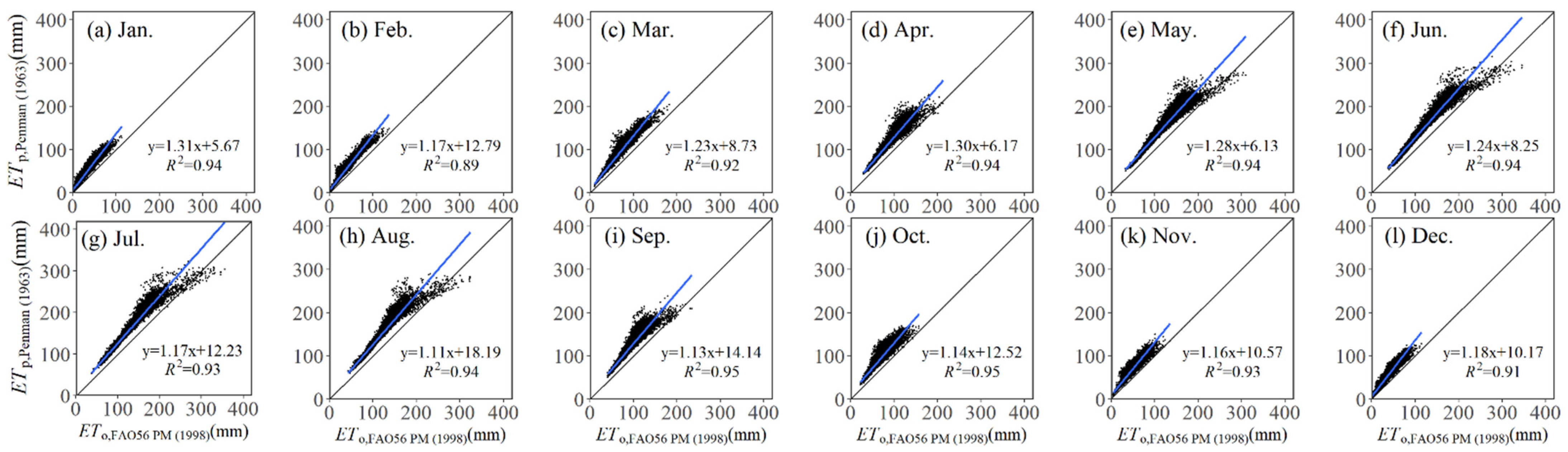
3.1.1. Temporal Differences

The temporal variations in the monthly ETp and ETo between 1961 and 2018 averaged from 551 sites across China are presented in Figure 3. The monthly ETp and ETo fluctuated periodically and their peaks and valleys varied synchronically. The monthly ETp were larger than the monthly ETo between 1961 and 2018. The monthly ETp and ETo differed clearly in their values.
To further show the value differences, the scatter plots of ETp and ETo between 1961 and 2018 in the 12 months of the year are shown in Figure 4. The monthly ETp and ETo ranged from 1 to 356 mm and from 2 to 323 mm, respectively. Most of the data-points were in the upper-left side of the 1:1 line, and some large values were in the upper-right part of the 1:1 line. These generally indicated a larger monthly ETp than ETo, especially in the cold months of November to March. The deviations of the monthly ETp from ETo were larger and increased with the increase in their values. Furthermore, the slopes of the linear function ranged between 1.11 and 1.30, indicating deviations of 11–30% from the monthly ETp to ETo. There were very high R2 values (0.89–0.95) representing a linear correlation between ETp and ETo, which confirmed the similarity in their patterns. Although there were slight differences in the R2 values of the cold months and warm months, this may be due to the variation in the meteorological data, which were using different weights in the two ET equations. Across the entire study area in each month, the relationship between the two was generally close.
The variations in long-term mean monthly ETp, ETo, and their differences D (=ETpET0) were also compared for the different sub-regions (Figure 5). The monthly ETp, ETo, and D showed peaks from around May to July. The peak values of ETp and ETo ranged from 144 to 218 mm and 116 to 176 mm for the sub-regions I to VII and for Mainland China, respectively. The peaks in the sub-regions ranked in the order of I > II > V > Mainland China > IV > VII > VI > III. The interannual variations in ETp and ETo were larger for the arid and semi-arid sub-regions (I and II) than the semi-humid and humid sub-regions (III, VI and VII). The monthly ETp were generally larger than the monthly ETo for the same month and the same region. The D values varied within the months of the year, reaching as high as 42 mm in July for the arid and semi-arid sub-region I.
Figure 3, Figure 4 and Figure 5 show that the monthly ETp was larger than ETo under most conditions. Although previous research has investigated the temporal variations in monthly ETp or ETo, seldom has research directly compared their values with the aim of differentiating the two variables.

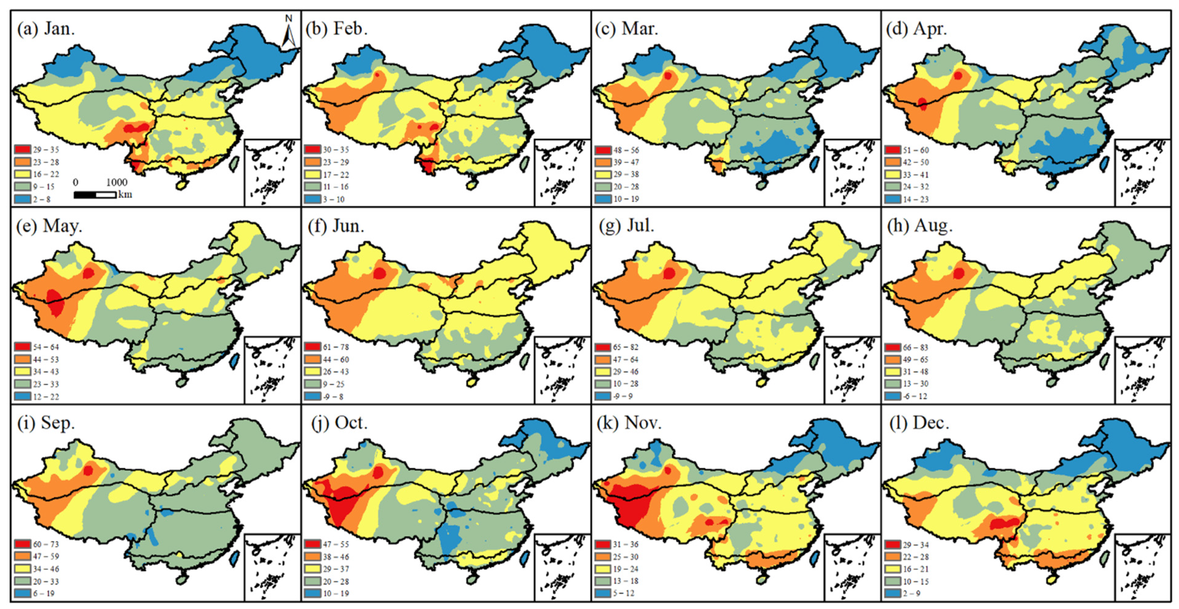
3.1.2. Spatial Differences

The spatial distribution of the long-term mean monthly D (=ETpETo) in the 12 months of the year (Figure 6) exhibited variable ranges between ETp and ETo across China. The results showed that: (1) The monthly D varied with the months. In cold and cool seasons (October to March), the smallest D values were in northeastern China and the areas of northwestern China. D values were mostly positive in mainland China, since the ETp values were generally larger than the ETo. (2) In the warm and hot seasons (April to September), the smallest D values were observed in southeastern or northeastern China. These were mostly positive but were occasionally negative, reaching as low as −9 mm month−1. The D values in sub-regions II (the Inner Mongolia grassland), III (the Qinghai–Tibetan Plateau), and V (northern China) were large. (3) In sub-region IV (northeastern China), the D values ranged between 2 and 33 mm month−1 in the year and did not change as much as other regions. (4) In general, the spatial distributions of the monthly D were both site- and region-specific.
The detailed differences in the D for the various sub-regions and months are presented in Table 1.

3.2. The Differences between Annual ETp and ETo

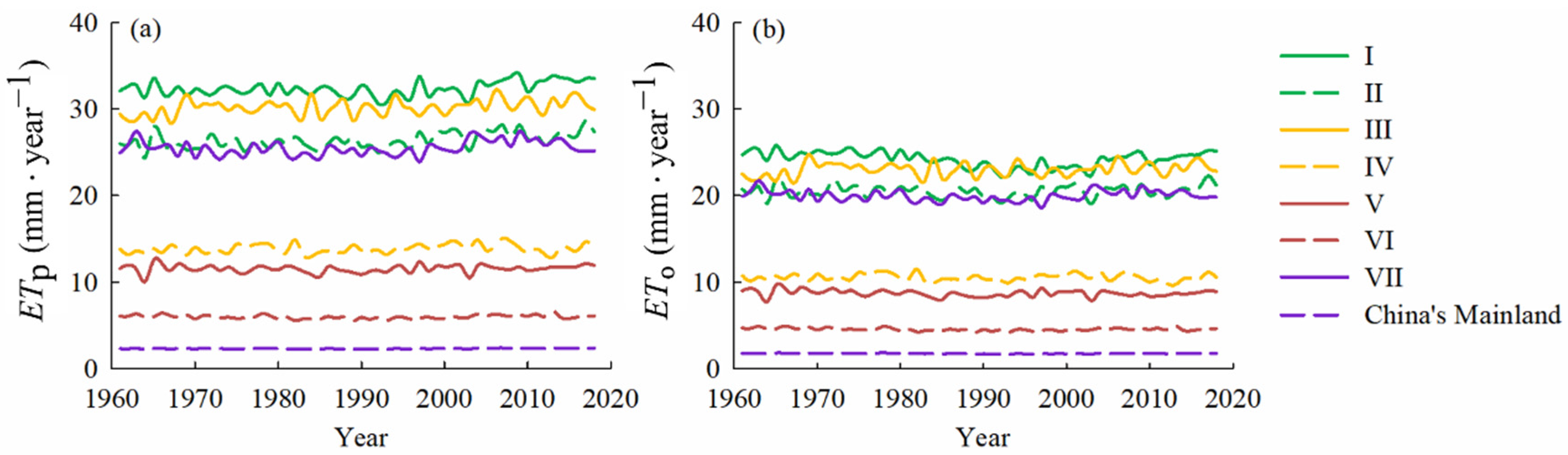
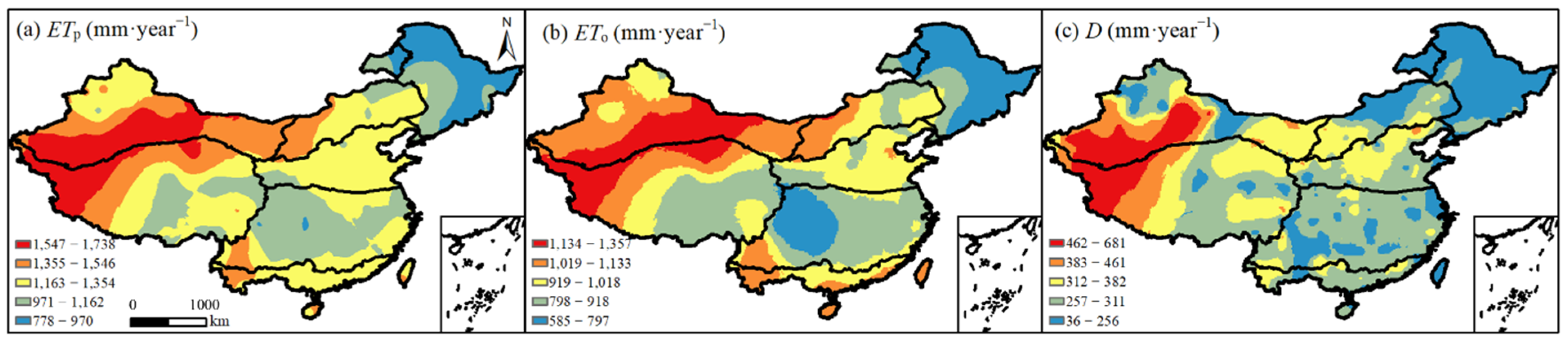
3.2.1. Temporal and Spatial Differences

The annual variations in the ETp and ETo in different sub-regions of China are presented in Figure 7. The fluctuating patterns of the ETp and ETo in the same sub-region were generally similar. The general sub-region ranks of the annual ETp and ETo values were sub-region I > III > II > VII > IV > V > VI > mainland China. The annual D values ranged from 256 mm to 315 mm for sub-regions I to VII and mainland China. It was observed that the annual ETp differed with the ETo and the differences varied within the different sub-regions.
The spatial distribution of the long-term mean annual ETp, ETo and D in mainland China are presented in Figure 8. The spatial distribution pattern of the annual ETp and ETo were similar; low values appeared in northeastern, central, and southern China, but large values appeared in northwestern and southern China. The ranges of the annual ETp and ETo differed from 778 to 1738 mm and from 585 to 1357 mm, respectively. The annual D values ranged from 36 to 681 mm and the highest values occurred in northwestern China and northern China. Therefore, in the areas with high D values, the differences in ETp and ETo should be considered in case their incorrect utilization should cause deviations.

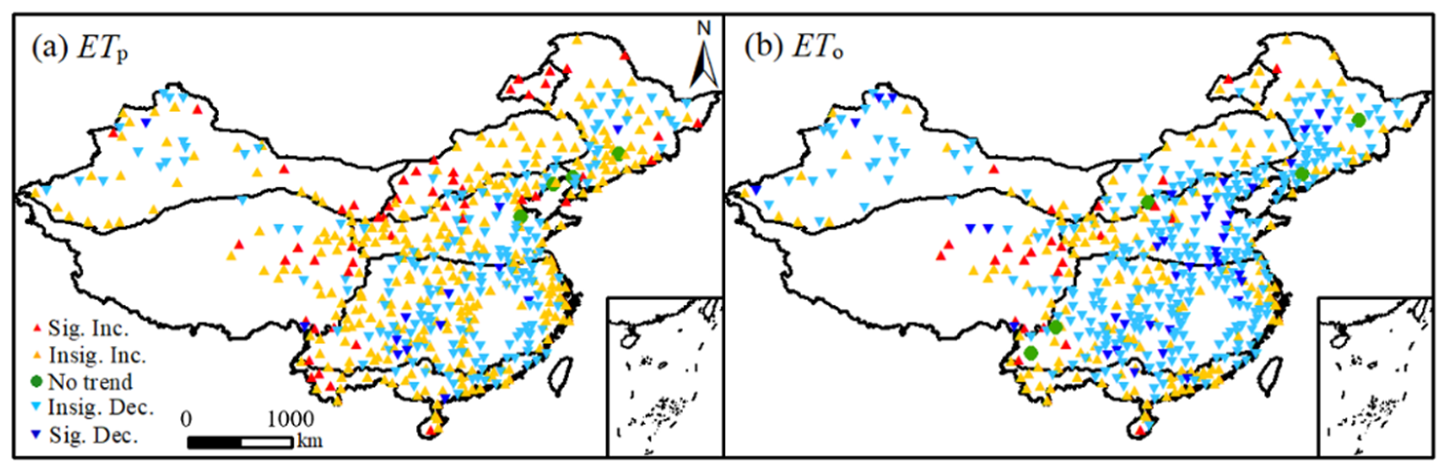
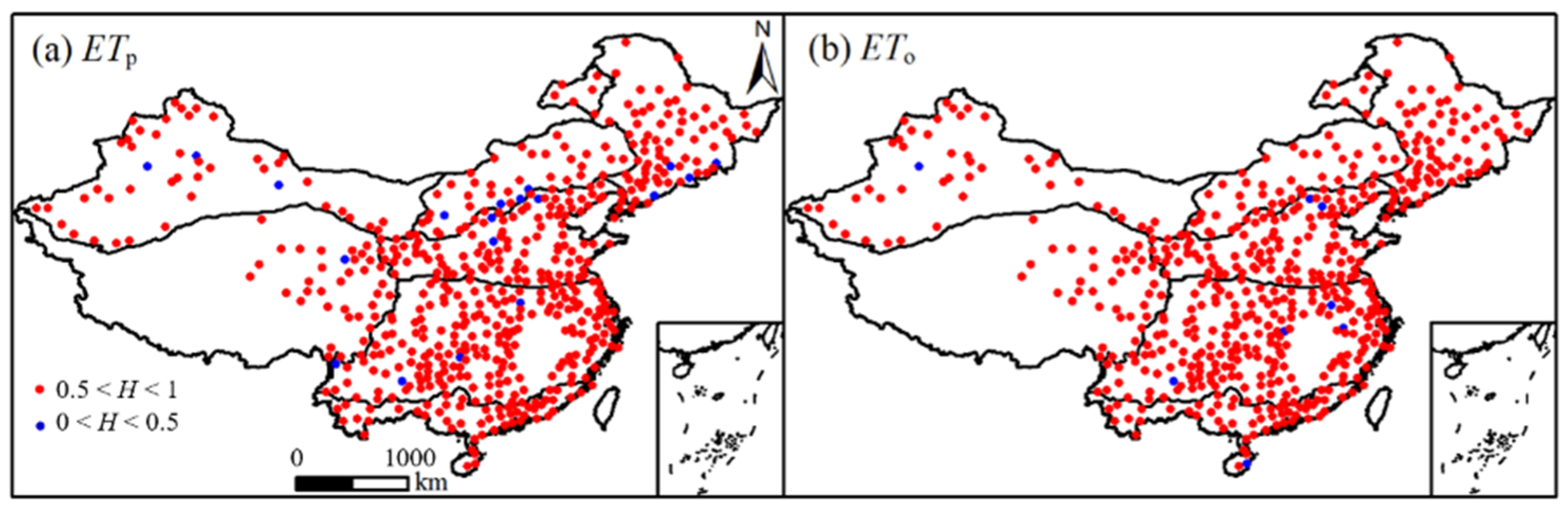
3.2.2. The Trends and Long—Term Dependence

To further compare the intrinsic features, the annual ETp and ETo for all the sites were mapped (Figure 9). Although the trend distribution of the annual ETp and ETo looked similar—namely, with more increasing trends seen in central, northern, and small areas of southern China—more sites had decreasing trends in their annual ETo. Their trend significance was also different.
The detailed numbers of the sites with different trends and significance are given in Table 2. In all the seven sub-regions, more sites had increasing trends in annual ETp than ETo. Thus, due to the differences in spatiotemporal distributions, the ETp and ETo must be used carefully and correctly in hydrology and meteorology research. Our results were different from those of Han et al. (2012), who investigated ETp trends between 1956 and 2005 at 244 sites in China and found decreasing ETp trends for 59.7%, 50%, and 64.2% of the total stations in the arid/semi-arid, semi-humid, and humid regions of China, respectively [51]. This was not surprising, since the studied station numbers and the studied period of the two were very different.
The spatial distributions of the Hurst index for the annual ETp and ETo were mapped and are presented in Figure 10. The detailed number of sites that had different ranges of the Hurst index in each sub-region are given in Table 3. The spatial distribution of the two terms were generally similar—namely, most sites had Hurst indices larger than 0.5. The sites that had different ranges of the Hurst index were also very close, but the number of ETp for H < 0.5 was almost 2.5 times that of ETo at 19 and 8 sites, respectively. This implied that the future ETp and ETo of most stations will maintain consistent with the previous trend, while several sites’ ETp and ETo will probably go in the opposite direction. When the Hurst index was combined with the result of the MMK test, the ETo trend of most sites showed an insignificant decrease, while a few sites’ ETo trend was reversed to increase in the future. In that situation, the trend of the ETp can be derived by comparing with the ETo.

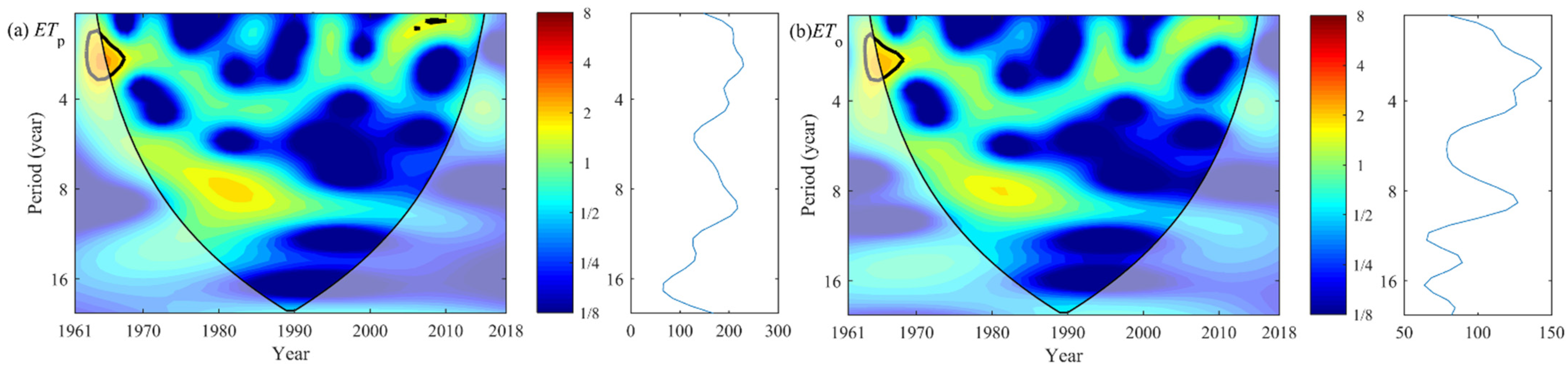
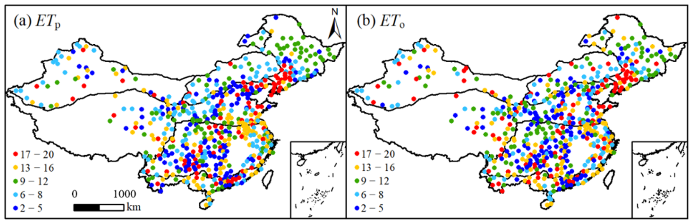
3.2.3. The Wavelet Periods

The variations in the wavelet spectrum and the wavelet variance for the annual ETp and ETo between 1961 and 2018 in mainland China are presented in Figure 11. The vibration intensity and fluctuation characteristics of the annual ETp and ETo were very similar. The primary and secondary periods of the annual ETp and ETo were almost same, being about 10 and 2 years, respectively, though somewhat weak. This was reasonable, since their annual variation patterns were very similar, although their values were very different (see Figure 7). Among the different time intervals, there were significant periods of four years between 1961 and 1970.
The spatial distributions of the primary periods in the annual ETp and ETo for all the studied sites are mapped and presented in Figure 12. In general, sites with shorter periods and with longer periods have similar distribution characteristics for both the annual ETp and ETo. They were mainly distributed in sub-regions V-VII, while a few were distributed in the other sub-regions.

4. Discussion

Though differentiating ETp and ETo seems easy, it is in fact very difficult and can greatly impact their further application. The standard method of the FAO-56 PM equation for ETo [6] has been universally accepted. However, no standard method for the ETp has been proposed. This research takes the Penman (1963) equation as the standard method for ETp, considering it is a combination-type equation and has generally good performance [25]. Moreover, several pieces of research found that the value of ETp was higher than that of ETo on a daily scale; for example, the root mean square errors between ETp and ETo were 1.88 mm/d and 0.93 mm/d in the Senegal River Valley and North China Plain, respectively [69,70]. These research specialized the wind effects and the dynamic process of vaporization by adding specific numbers to represent the study area. However, this is still not a universal method. The Thornthwaite (1948) equation is also used to calculate ETp, requiring only temperature data [23]. However, it tends to underestimate ETp in humid regions [71,72]. There may be other better ETp equations used in different countries. Nevertheless, there are apparent differences, especially in the spatiotemporal variations, between the ETp and ETo, at monthly, annual, and other timescales.
Since the monthly and annual values, ranges, seasonal changes, spatial distributions, long-term dependent characteristics, periods, trends, and significance of ETp and ETo differed at most of the sites in the sub-regions and in mainland China, in the future the unitization of the two terms should be approached more carefully. Not only do the quantitative characteristics of ETp and ETo differ, but the application scale differs as well. ETp has been suitably applied to studies with a larger spatial scale, including the rainfall-runoff modeling of many catchments [39], discharge projections [73], and the attribution of evapotranspiration changes under non-water-limited conditions [15], as well as drought severity analysis on a regional, national and global scale [74,75,76]. Comparatively, ETo is applied on smaller spatial scales, including site, field, and regional scales [43,44,46,47,49].
In addition, there was variability in the D series on the monthly and yearly timescales, as clearly shown by Anselin Local Moran’s I index [77] (Table 4, Figures S1 and S2). More studies are needed for detailed descriptions. It is easy to see that the major Moran’s type of D series is not significant, that there is a high proportion of High-High (HH) or Low-Low (LL) clusters in the rest sites, and that there are only a few sites representing the High-Low (HL) or Low-High (LH) outlier. The Moran’s type spatial distribution of monthly and yearly D also depicted a similar annual trend showing that the HH or LL sites’ position will reverse to each other in a year (Figures S1 and S2).

5. Conclusions

The differences between ETp and ETo at monthly and annual timescales in China were studied between 1961 and 2018. At most sites in most months, the ETp was larger than the ETo. Except for some similarity in the long-term dependence indicated by the Hurst index and the spatial distribution of the primary period calculated by wavelet analysis, generally there were many differences between the ETp and ETo.
At different timescales, ETp and ETo showed some similar situations and some different behaviors. Their values were closer in some months than in others because of the lower influence of the surface resistance of evapotranspiration in the calculation equations. Different spatial distributions in various sub-regions and mainland China were found. These were related to the variation in weather data under different situations. As for the monthly ETp and ETo, at most of the sites in every sub-region, the ETp was higher than the ETo. This result provides supportive guidance for the related policy managers to deal with water risk management. The maximum difference was observed in May or July, and the minimum difference was observed in December or January. Different distribution trends of ETp and ETo were also shown. On the annual scale, the ETp and ETo showed a similar spatial distribution but different quantities, and there was an obvious difference in the significance, future trend, and primary periods at all stations. This confirmed the discrepancy of the spatial–temporal variations between ETp and ETo. Overall, our results strongly indicate that researchers should use ETp and ETo carefully and be sure to differentiate them.

Supplementary Materials

The following supporting information can be downloaded at: https://www.mdpi.com/article/10.3390/w14060988/s1, Figure S1: The Anselin Local Moran's I index distribution of monthly D; Figure S2: The Anselin Local Moran's I index distribution of yearly ETp, ETo and D respectively.

Author Contributions

Conceptualization, K.X., X.Z. and Y.L.; Methodology, K.X.; Software, K.X.; Validation, X.P. and N.Y.; Original draft preparation writing, K.X. and Y.L.; Review and Editing, A.B., D.L.L., F.L., Y.Z., B.P. and F.L. All authors have read and agreed to the published version of the manuscript.

Funding

This research was funded by National Key Research and Development Program of China (2019YFA0606902), the Science and Technology Project of Tumushuk, Third Division (No. S202102GG018); and the National Natural Science Foundation of China (No. 52079114).

Informed Consent Statement

Informed consent was obtained from all subjects involved in the study.

Data Availability Statement

The weather data can be found from China Meteorological Data Sharing center (http://data.cma.cn/ (accessed on 8 February 2022)).

Conflicts of Interest

The authors declare no conflict of interest.

Abbreviations

ETp—potential evapotranspiration; ETo—reference crop evapotranspiration; R2—coefficient of determination; FAO—Food and Agriculture Organization; R/S—rescaled; MMK—modified Mann–Kendall.

References

  1. Milly, P.C.D.; Dunne, K.A. Potential evapotranspiration and continental drying. Nat. Clim. Change 2016, 6, 946–949. [Google Scholar] [CrossRef]
  2. Peng, L.; Li, Y.; Feng, H. The best alternative for estimating reference crop evapotranspiration in different sub-regions of mainland China. Sci. Rep. 2017, 7, 5458. [Google Scholar] [CrossRef] [PubMed] [Green Version]
  3. Vörösmarty, C.J.; Federer, C.A.; Schloss, A.L. Potential evaporation functions compared on US watersheds: Possible implications for global-scale water balance and terrestrial ecosystem modeling. J. Hydrol. 1998, 207, 147–169. [Google Scholar] [CrossRef]
  4. Yao, N.; Li, Y.; Dong, Q.G.; Li, L.; Peng, L.; Feng, H. Influence of the accuracy of reference crop evapotranspiration on drought monitoring using standardized precipitation evapotranspiration index in mainland China. Land. Degrad. Dev. 2020, 31, 266–282. [Google Scholar] [CrossRef]
  5. Zhang, Y. Estimation of Potential Evapotranspiration by Different Methods in Handan Eastern Plain, China. Water Sci. Eng. 2019, 4, 117. [Google Scholar]
  6. Allen, R.G.; Pereira, L.S.; Raes, D.; Smith, M. Crop evapotranspiration: Guidelines for computing crop water requirements. In Irrigation and Drainage Paper No 56; Food and Agriculture Organization of the United Nations (FAO): Rome, Italy, 1998. [Google Scholar]
  7. Ohana-Levi, N.; Ben-Gal, A.; Munitz, S.; Netzer, Y. Grapevine crop evapotranspiration and crop coefficient forecasting using linear and non-linear multiple regression models. Agric. Water Manag. 2022, 262, 107317. [Google Scholar] [CrossRef]
  8. Hu, K.; Awange, J.; Kuhn, M.; Zerihun, A. Irrigated agriculture potential of Australia’s northern territory inferred from spatial assessment of groundwater availability and crop evapotranspiration. Agric. Water Manag. 2022, 264, 107466. [Google Scholar] [CrossRef]
  9. Gentilucci, M.; Barbieri, M.; Burt, P. (Eds.) Climate and territorial suitability for the Vineyards developed using GIS techniques. In Proceedings of the Conference of the Arabian Journal of Geosciences, Sousse, Tunisia, 2–5 November 2018. [Google Scholar]
  10. Saadi, S.; Todorovic, M.; Tanasijevic, L.; Pereira, L.S.; Pizzigalli, C.; Lionello, P. Climate change and Mediterranean agriculture: Impacts on winter wheat and tomato crop evapotranspiration, irrigation requirements and yield. Agric. Water Manag. 2015, 147, 103–115. [Google Scholar] [CrossRef]
  11. Fan, J.; Wu, L.; Zhang, F.; Xiang, Y.; Zheng, J. Climate change effects on reference crop evapotranspiration across different climatic zones of China during 1956–2015. J. Hydrol. 2016, 542, 923–937. [Google Scholar] [CrossRef]
  12. Saray, M.H.; Eslamian, S.S.; Klove, B.; Gohari, A. Regionalization of potential evapotranspiration using a modified region of influence. Theor. Appl. Climatol. 2019, 140, 115–127. [Google Scholar] [CrossRef] [Green Version]
  13. Silva, C.R.D.; Barbosa, L.A.; Finzi, R.R.; Riberio, B.T.; Dias, N.D.S. Accuracy of air temperature forecasts and its use for prediction of the reference evapotranspiration. Biosci. J. 2020, 36, 17–22. [Google Scholar] [CrossRef]
  14. Um, M.; Kim, Y.; Park, D.; Jung, K.; Wang, Z.; Kim, M.M.; Shin, H. Impacts of potential evapotranspiration on drought phenomena in different regions and climate zones. Sci. Total Environ. 2020, 703, 135590. [Google Scholar] [CrossRef] [PubMed]
  15. Yang, Y.; Roderick, M.L.; Zhang, S.; Mcvicar, T.R.; Donohue, R.J. Hydrologic implications of vegetation response to elevated CO2 in climate projections. Nat. Clim. Change 2019, 9, 44–48. [Google Scholar] [CrossRef]
  16. Li, J.; Wu, C.; Wang, X.; Peng, J.; Dong, D.; Lin, G.; Gonsamo, A. Satellite observed indicators of the maximum plant growth potential and their responses to drought over Tibetan Plateau (1982–2015). Ecol. Indic. 2020, 108, 105732. [Google Scholar] [CrossRef]
  17. Zhao, J.; Wang, Z. Future trends of water resources and influences on agriculture in China. PLoS ONE 2020, 15, e0231671. [Google Scholar] [CrossRef]
  18. Shanmugam, M.; Mekonnen, M.; Ray, C. Grid-Based Model for Estimating Evapotranspiration Rates of Heterogeneous Land Surface. J. Irrig. Drain. Eng. 2020, 146, 04019030. [Google Scholar] [CrossRef]
  19. Malik, A.; Kumar, A.; Ghorbani, M.A.; Kashani, M.H.; Kisi, O.; Kim, S. The viability of co-active fuzzy inference system model for monthly reference evapotranspiration estimation: Case study of Uttarakhand State. Hydrol. Res. 2019, 50, 1623–1644. [Google Scholar] [CrossRef] [Green Version]
  20. You, G.; Arain, M.A.; Wang, S.; Lin, N.; Wu, D.; Mckenzie, S.; Zou, C.; Liu, B.; Zhang, X.; Gao, J. Trends of actual and potential evapotranspiration based on Bouchet’s complementary concept in a cold and arid steppe site of Northeastern Asia. Agr. For. Meteorol. 2019, 279, 107684. [Google Scholar] [CrossRef]
  21. Adhikari, A.; Mainali, K.P.; Rangwala, I.; Hansen, A.J. Various measures of potential evapotranspiration have species-specific impact on species distribution models. Ecol. Model. 2019, 414, 108836. [Google Scholar] [CrossRef]
  22. Guo, D.; Westra, S.; Maier, H.R. An R package for modelling actual, potential and reference evapotranspiration. Environ. Model. Softw. 2016, 78, 216–224. [Google Scholar] [CrossRef]
  23. Thornthwaite, C.W. An Approach toward a Rational Classification of Climate. Geogr. Rev. 1948, 38, 55–94. [Google Scholar] [CrossRef]
  24. Penman, H.L. Evaporation: An introductory survey. Neth. J. Agri. Sci. 1956, 4, 9–29. [Google Scholar] [CrossRef]
  25. Penman, H.L. (Ed.) Vegetation and Hydrology, Tech. Commun. 53, Commonwealth Bureau of Soils; Soil Science: Harpenden, UK, 1963. [Google Scholar]
  26. Anon, J. Proceeding of the informal meeting on physics in agriculture. Neth. J. Agri. Sci. 1956, 4, 162–175. [Google Scholar]
  27. WMO. Sites for Wind-Power Installations; WMO No. 156, Technical Note No. 63; WMO: Geneva, Switzerland, 1963; Available online: https://library.wmo.int/index.php?lvl=notice_display&id=5475#.YjfmEHpBzDc (accessed on 8 February 2022).
  28. Jensen, M.E. Water Consumption by Agricultural Plants. In Plant Water Consumption & Response. Volume II. Water Deficits and Plant Growth; Kozlowski, T.T., Ed.; Academic Press: New York, NY, USA; London, UK, 1968; pp. 1–22. [Google Scholar]
  29. Granger, R.J. An examination of the concept of potential evaporation. J. Hydrol. 1989, 111, 9–19. [Google Scholar] [CrossRef]
  30. Doorenbos, J.; Pruitt, W. Guidelines for Predicting Crop Water Requirements, Irrigation and Drainage Paper No. 24; FAO: Rome, Italy, 1977. [Google Scholar]
  31. Ochoa-Sánchez, A.; Crespo, P.; Carrillo-Rojas, G.; Sucozhañay, A.; Célleri, R. Actual Evapotranspiration in the High Andean Grasslands: A Comparison of Measurement and Estimation Methods. Front. Earth Sci. 2019, 7, 55. [Google Scholar] [CrossRef] [Green Version]
  32. Chen, S.; Liu, Y.; Axel, T. Climatic change on the Tibetan Plateau: Potential Evapotranspiration Trends from 1961–2000. Clim. Change 2006, 76, 291–319. [Google Scholar]
  33. Seiller, G.; Anctil, F. How do potential evapotranspiration formulas influence hydrological projections? Hydrolog. Sci. J. 2016, 61, 2249–2266. [Google Scholar] [CrossRef] [Green Version]
  34. Sun, C.; Zheng, Z.; Chen, W.; Wang, Y. Spatial and Temporal Variations of Potential Evapotranspiration in the Loess Plateau of China during 1960–2017. Sustainability 2020, 12, 354. [Google Scholar] [CrossRef] [Green Version]
  35. Sun, S.; Lei, S.; Jia, H.; Li, C.; Zhang, J.; Meng, P. Tree-Ring Analysis Reveals Density-Dependent Vulnerability to Drought in Planted Mongolian Pines. Forests 2020, 11, 98. [Google Scholar] [CrossRef] [Green Version]
  36. Gwate, O.; Mantel, S.K.; Palmer, A.R.; Gibson, L.; Munch, Z. Measuring and modelling evapotranspiration in a South African grassland: Comparison of two improved Penman-Monteith formulations. Water SA 2018, 44, 482–494. [Google Scholar] [CrossRef] [Green Version]
  37. Lewis, C.S.; Allen, L.N. Potential Crop Evapotranspiration and Surface Evaporation Estimates via a Gridded Weather Forcing Dataset. J. Hydrol. 2017, 546, 450–463. [Google Scholar] [CrossRef] [Green Version]
  38. Ding, H.; Xingming, H.; Ying, H.; Jingxiu, Q. Uncertainty assessment of potential evapotranspiration in arid areas, as estimated by the Penman-Monteith method. J. Arid. Land 2020, 12, 166–180. [Google Scholar]
  39. Oudin, L.; Hervieu, F.; Michel, C.; Perrin, C.; Andreassian, V.; Anctil, F.; Loumagne, C. Which potential evapotranspiration input for a lumped rainfall-runoff model? Part 2: Towards a simple and efficient potential evapotranspiration model for rainfall-runoff modelling. J. Hydrol. 2005, 303, 290–306. [Google Scholar] [CrossRef]
  40. Jensen, M.E.; Burman, R.D.; Allen, R.G. Evapotranspiration and Irrigation Water Requirements; Agriculture Society Civil Engineering: New York, NY, USA, 1990. [Google Scholar]
  41. Hargreaves, G.H.; Samani, Z.A. Estimating potential evapotranspiration. J. Irrig. Drain. Div. 1982, 108, 225–230. [Google Scholar] [CrossRef]
  42. Hargreaves, G.H.; Samani, Z.A. Reference crop evapotranspiration from temperature. Appl. Eng. Agric. 1985, 1, 96–99. [Google Scholar] [CrossRef]
  43. Dinpashoh, Y.; Jhajharia, D.; Fakheri-Fard, A.; Singh, V.P.; Kahya, E. Trends in reference crop evapotranspiration over Iran. J. Hydrol. 2011, 399, 422–433. [Google Scholar] [CrossRef]
  44. Feng, Y.; Cui, N.; Zhao, L.; Hu, X.; Gong, D. Comparison of ELM, GANN, WNN and empirical models for estimating reference evapotranspiration in humid region of Southwest China. J. Hydrol. 2016, 536, 376–383. [Google Scholar] [CrossRef]
  45. Gong, L.; Xu, C.; Chen, D.; Halldin, S.; Chen, Y.D. Sensitivity of the Penman–Monteith reference evapotranspiration to key climatic variables in the Changjiang (Yangtze River) basin. J. Hydrol. 2006, 329, 620–629. [Google Scholar] [CrossRef]
  46. Hargreaves, G.H.; Allen, R.G. History and evaluation of Hargreaves evapotranspiration equation. J. Irrig. Drain. Eng. 2003, 129, 53–63. [Google Scholar] [CrossRef]
  47. Li, Z.; Zheng, F.; Liu, W. Spatiotemporal characteristics of reference evapotranspiration during 1961–2009 and its projected changes during 2011–2099 on the Loess Plateau of China. Agr. For. Meteorol. 2012, 154, 147–155. [Google Scholar] [CrossRef]
  48. Mcvicar, T.R.; Van Niel, T.G.; Li, L.; Hutchinson, M.F.; Mu, X.; Liu, Z. Spatially distributing monthly reference evapotranspiration and pan evaporation considering topographic influences. J. Hydrol. 2007, 338, 196–220. [Google Scholar] [CrossRef]
  49. Tabari, H.; Marofi, S.; Aeini, A.; Talaee, P.H.; Mohammadi, K. Trend analysis of reference evapotranspiration in the western half of Iran. Agr. For. Meteorol. 2011, 151, 128–136. [Google Scholar] [CrossRef]
  50. Chattopadhyay, N.; Hulme, M. Evaporation and potential evapotranspiration in India under conditions of recent and future climate change. Agr. For. Meteorol. 1997, 87, 55–73. [Google Scholar] [CrossRef]
  51. Han, S.; Xu, D.; Wang, S. Decreasing potential evaporation trends in China from 1956 to 2005: Accelerated in regions with significant agricultural influence? Agr. For. Meteorol. 2012, 154, 44–56. [Google Scholar] [CrossRef]
  52. Wang, K.; Xu, Q.; Li, T. Does recent climate warming drive spatiotemporal shifts in functioning of high-elevation hydrological systems? Sci. Total Environ. 2020, 719, 137507. [Google Scholar] [CrossRef]
  53. Katerji, N.; Rana, G. Crop reference evapotranspiration: A discussion of the concept, analysis of the process and validation. Water Resour. Manag. 2011, 25, 1581–1600. [Google Scholar] [CrossRef]
  54. Xiang, K.; Li, Y.; Horton, R.; Feng, H. Similarity and difference of potential evapotranspiration and reference crop evapotranspiration -a review. Agric. Water Manag. 2020, 232, 106043. [Google Scholar] [CrossRef]
  55. Helsel, D.R.; Hirsch, R.M. Statistical Methods in Water Resources; Elsevier: Amsterdam, The Netherland, 1992. [Google Scholar]
  56. Ayantobo, O.O.; Li, Y.; Song, S.; Yao, N. Spatial comparability of drought characteristics and related return periods in mainland China over 1961–2013. J. Hydrol. 2017, 550, 549–567. [Google Scholar] [CrossRef]
  57. Yao, N.; Li, Y.; Lei, T.; Peng, L. Drought evolution, severity and trends in mainland China over 1961–2013. Sci. Total Environ. 2018, 616, 73–89. [Google Scholar] [CrossRef]
  58. Li, S.; Kang, S.; Zhang, L.; Zhang, J.; Du, T.; Tong, L.; Ding, R. Evaluation of six potential evapotranspiration models for estimating crop potential and actual evapotranspiration in arid regions. J. Hydrol. 2016, 543, 450–461. [Google Scholar] [CrossRef]
  59. Xu, K.; Yang, D.; Yang, H.; Li, Z.; Qin, Y.; Shen, Y. Spatio-temporal variation of drought in China during 1961–2012: A climatic perspective. J. Hydrol. 2015, 526, 253–264. [Google Scholar] [CrossRef]
  60. Yang, Y.; Chen, R.; Song, Y.; Han, C.; Liu, J.; Liu, Z. Sensitivity of potential evapotranspiration to meteorological factors and their elevational gradients in the Qilian Mountains, northwestern China. J. Hydrol. 2019, 568, 147–159. [Google Scholar] [CrossRef]
  61. Yue, S.; Wang, C.Y. Regional Streamflow Trend Detection with Consideration of Both Temporal and Spatial Correlation. Int. J. Climatol. 2002, 22, 933–946. [Google Scholar] [CrossRef]
  62. Mann, H.B. Nonparametric Tests against Trend. Econometrica 1945, 13, 245–259. [Google Scholar] [CrossRef]
  63. Kendall, M.G. Rank Auto Correlation Methods. Brit. J. Psychol. 1976, 25, 86–97. [Google Scholar]
  64. Li, Y.; Horton, R.; Ren, T.; Chen, C. Prediction of annual reference evapotranspiration using climatic data. Agric. Water Manag. 2010, 97, 300–308. [Google Scholar] [CrossRef]
  65. Mandelbrot, B.B.; Wallis, J.R. Robustness of the rescaled range R/S in the measurement of noncyclic long run statistical dependence. Water Resour. Res. 1969, 5, 967–988. [Google Scholar] [CrossRef]
  66. Hurst, H.E. Long-term storage capacity of reservoirs. Trans. Am. Soc. Civil. Eng. 1951, 116, 770–808. [Google Scholar] [CrossRef]
  67. Liu, Y.; Li, Y.; Li, L.; Chen, C. Spatiotemporal Variability of Monthly and Annual Snow Depths in Xinjiang, China over 1961–2015 and the Potential Effects. Water 2019, 11, 1666. [Google Scholar] [CrossRef] [Green Version]
  68. Li, L.; Yao, N.; Li, Y.; Liu, D.L.; Wang, B.; Ayantobo, O.O. Future projections of extreme temperature events in different sub-regions of China. Atmos. Res. 2019, 217, 150–164. [Google Scholar] [CrossRef]
  69. Djaman, K.; Balde, A.B.; Sow, A.; Muller, B.; Irmak, S.; N’Diaye, M.K.; Manneh, B.; Moukoumbi, Y.D.; Futakuchi, K.; Saito, K. Evaluation of sixteen reference evapotranspiration methods under sahelian conditions in the Senegal River Valley. J. Hydrol. 2015, 3, 139–159. [Google Scholar] [CrossRef] [Green Version]
  70. Liu, X.; Xu, C.; Zhong, X.; Li, Y.; Yuan, X.; Cao, J. Comparison of 16 models for reference crop evapotranspiration against weighing lysimeter measurement. Agric. Water Manag. 2017, 184, 145–155. [Google Scholar] [CrossRef]
  71. Sentelhas, P.C.; Gillespie, T.J.; Santos, E.A. Evaluation of FAO Penman–Monteith and alternative methods for estimating reference evapotranspiration with missing data in Southern Ontario, Canada. Agric. Water Manag. 2010, 97, 635–644. [Google Scholar] [CrossRef]
  72. Valipour, M.; Sefidkouhi, M.A.G.; Raeini, M. Selecting the best model to estimate potential evapotranspiration with respect to climate change and magnitudes of extreme events. Agric. Water Manag. 2017, 180, 50–60. [Google Scholar] [CrossRef]
  73. Dakhlaoui, H.; Seibert, J.; Hakala, K. Sensitivity of discharge projections to potential evapotranspiration estimation in Northern Tunisia. Reg. Environ. Change 2020, 20, 34. [Google Scholar] [CrossRef] [Green Version]
  74. Burke, E.J.; Brown, S.I.J.; Christidis, N. Modeling the Recent Evolution of Global Drought and Projections for the Twenty-First Century with the Hadley Centre Climate Model. J. Hydrometeorol. 2006, 7, 1113–1125. [Google Scholar] [CrossRef]
  75. Li, Y.; Sun, C. Impacts of the superimposed climate trends on droughts over 1961–2013 in Xinjiang, China. Theor. Appl. Climatol. 2017, 129, 977–994. [Google Scholar] [CrossRef]
  76. Yao, N.; Li, L.; Feng, P.; Feng, H.; Liu, D.L.; Liu, Y.; Jiang, K.; Hu, X.; Li, Y. Projections of drought characteristics in China based on a standardized precipitation and evapotranspiration index and multiple GCMs. Sci. Total Environ. 2020, 704, 135245. [Google Scholar] [CrossRef]
  77. Anselin, L. Local indicators of spatial association—LISA. Geogr. Anal. 1995, 27, 93–115. [Google Scholar] [CrossRef]
Figure 1. The digital evaluation of the sub-region divisions and the distribution of the weather stations. (a) Sub-region division and elevation; (b) Meteorological station.
Water 14 00988 g001
Figure 2. Flow chart of the study framework used for this research.
Water 14 00988 g002
Figure 3. The variations in monthly ETo and ETp averaged from 551 sites in mainland China.
Water 14 00988 g003
Figure 4. The scatter plots of monthly ETo and ETp for the 12 months (containing 551 sites).
Water 14 00988 g004
Figure 5. The long-term mean monthly variables averaged from the sites of different sub-regions. (a) ETo, (b) ETp and (c) D.
Water 14 00988 g005
Figure 6. The spatial distribution of the long-term mean monthly D in mainland China (the site values were interpolated by the Kriging method in ArcGIS 10.3).
Water 14 00988 g006
Figure 7. The temporal variations in annual variables in different sub-regions of China. The sub-regional ETp and ETo values were computed using the site-specific weight coefficients obtained from the Theson-polygon method in ArcGis. (a) ETp and (b) ETo.
Water 14 00988 g007
Figure 8. The spatial distribution of longterm mean annual (a) ETp, (b) ETo, and (c) D in mainland China.
Water 14 00988 g008
Figure 9. The trends and significance of annual ETp and ETo in mainland China.
Water 14 00988 g009
Figure 10. The spatial distribution of the Hurst index denoting the long-term dependence of ETp and ETo.
Water 14 00988 g010
Figure 11. The wavelet spectrum and wavelet variance for the annual ETp (a) and ETo (b) of mainland China. The thin solid lines denote the cones of influence, and the thick solid lines show the 95% confidence levels. The color bar represents the vibration intensity of the periods at different timescales.
Water 14 00988 g011
Figure 12. The main periods of annual ETp (a) and ETo (b) extracted from wavelet analysis.
Water 14 00988 g012
Table 1. Values of the monthly D in different sub-regions and months. Unit: mm month−1.
MonthSub-Region
IIIIIIIVVVIVII
January151192061616
February1515122081716
March22262127172521
April27342830243024
May31393432313527
June30403629313525
July30423529273028
August29423328262928
September27383024262824
October24312424202623
November18191422111919
December1612102171618
Table 2. The station numbers of annual ETo and ETp, which had different trends and levels of significance in different sub-regions.
TermTrendSub-RegionSubtotal
IIIIIIIVVVIVII
ETPSignificant increase
Insignificant increase
3522825550
232419365511729303
No trend00000404
Insignificant decrease20151628414318181
Significant decrease032341013
ET0Significant increase0102514325
Insignificant increase1716924346016176
No trend00001405
Insignificant decrease272725366010030305
Significant decrease2357812340
Table 3. The station numbers of the Hurst coefficient for annual ETo and ETp in different sub-regions.
Sub-RegionIIIIIIIVVVIVIISubtotal
ETP0.5 < H < 14343386510518652532
0 < H < 0.5341434019
ET00.5 < H < 14547396910618651543
0 < H < 0.510002418
Table 4. The site numbers of Anselin Local Moran’s I index for D series.
TimesclaeMonthlyYearly
Moran’s IJanuaryFebruary MarchAprilMayJuneJulyAuguestSeptemberOctoberNovemberDecember
NS338370342337328285406435407391367341383
HH977896958810263486167768979
HL0134433323113
LH2478766565537
LL114981031071241557360758510211779
Notes: NS: not significant; HH: High-High Cluster; HL: High-Low Outlier; LH: Low-High Outlier; LL: Low-Low Cluster.
Publisher’s Note: MDPI stays neutral with regard to jurisdictional claims in published maps and institutional affiliations.

