Article

Refinements and Analysis of the Optical-Microwave Scintillometry Method Applied to Measurements over a Vineyard in Chile

by
Francisca Aguirre
1,2,
Oscar Hartogensis
3,
Francisco Meza
4,5 and
Francisco Suárez
1,2,6,*
1
Departamento de Ingeniería Hidráulica y Ambiental, Pontificia Universidad Católica de Chile, Santiago 7820436, Chile
2
Centro de Excelencia en Geotermia de los Andes (CEGA), Santiago 7820436, Chile
3
Meteorology and Air Quality, Wageningen University and Research, 6700 AA Wageningen, The Netherlands
4
Departamento de Ecosistemas y Medio Ambiente, Pontificia Universidad Católica de Chile, Santiago 7820436, Chile
5
Centro Interdisciplinario de Cambio Global, Pontificia Universidad Católica de Chile, Santiago 7820436, Chile
6
Centro de Desarrollo Urbano Sustentable (CEDEUS), Santiago 7820436, Chile
*
Author to whom correspondence should be addressed.
Water 2022, 14(3), 474; https://doi.org/10.3390/w14030474
Submission received: 31 December 2021 / Revised: 2 February 2022 / Accepted: 3 February 2022 / Published: 5 February 2022
(This article belongs to the Special Issue Evapotranspiration Measurements and Modeling)

Abstract

:
Evapotranspiration (ET) is a critical component of the hydrological cycle, and it links water and energy budgets in the form of latent heat (LvE) released into the atmosphere. However, ET is difficult to measure and is not always well described in arid regions. Thus, novel techniques are required for its accurate measurement. Scintillometers are an interesting alternative for traditional methods, such as Eddy Covariance systems (EC). Scintillometer studies have reported good results, but their signals can present unwanted contributions that result in incorrect heat fluxes. In this study, scintillometer data showed unrealistic heat flux values, and thus, the data were reprocessed through spectral analysis to eliminate unwanted contributions from electronic noise, absorption, and tripod vibrations using a new proposed data cleaning method. After performing the spectral cleaning method, scintillometer-based heat fluxes were calculated using several methods: (i) the standalone LAS method, (ii) Hill model, (iii) Lüdi et al. model, and (iv) a hybrid model between Hill and Lüdi et al. Furthermore, a Monin–Obukhov similarity theory (MOST) analysis was performed to evaluate the fluxes’ sensitivity to the choice of the similarity functions. Corrected sensible heat flux (H) estimations agreed well with those obtained with an EC system. However, considerable differences were found for LvE (and, consequently, ET). The Lüdi et al. model LvE estimates were closer to those obtained with the EC system, overestimating it by 14%, with a correlation slope of 1.07, R2 = 0.91, and a Nash-Sutcliffe efficiency of 0.90. Furthermore, it was found that using different Monin–Obukhov similarity functions resulted in more than ±12% of difference on the estimated LvE. For future works, it is strongly recommended to apply the proposed spectral cleaning method as it greatly improves scintillometer data.

1. Introduction

Evapotranspiration (ET) is a critical component of the hydrological cycle, but it is not always well characterized in arid and semi-arid regions [1,2,3]. ET links water and energy budgets via latent heat (LvE) released to the atmosphere, and its measurements are difficult to obtain. Therefore, studies have investigated different methods to obtain proper ET estimates [1,4,5,6,7].
Recent studies have shown that scintillometers are an interesting alternative to traditional methods, such as Eddy Covariance systems (EC) [8,9,10], especially for natural landscapes, and for estimating area-averaged sensible heat (H) and LvE over spatial scales that range from 0.1 to larger scales such as 10 km [11,12,13]. Scintillometers’ functioning consists of a receiver that measures signal variances from an electromagnetic beam sent by a transmitter installed at a certain distance, known as the path length. This system allows computing heat fluxes by combining theoretical principles of atmospheric turbulence with the physics of electromagnetic wave propagation and by applying the Monin–Obukhov similarity theory (MOST [14]). To compute ET from scintillometer measurements, various approaches can be followed, such as the Large Aperture Scintillometer (LAS) energy balance closure (EBC) method [15] (herein referred to as the standalone LAS method), the Hill’s [16] method, the Lüdi et al. [17] method, and a hybrid method between Hill and Lüdi [18].
Scintillometer technology overcomes many of the limitations of EC systems, as it does not suffer from flow distortion (by the mast or the instrument itself) [12], it obtains representative fluxes for larger scales, and it has been successfully used in heterogeneous terrains [19]. However, its main disadvantages are that (1) H and LvE are determined indirectly; (2) scintillometer signals usually present unwanted contributions from absorption and tripod vibrations and, sometimes, from electronic noise at high frequencies [18,20]; and (3) there are several MOST universal similarity functions [21]. Hence, proper selection of these functions for each study site is important for a correct estimation of H and LvE.
Absorption contributions occur due to air masses that pass slowly through the scintillometer trajectory, creating a fluctuation that is slow compared to turbulence, while electronic noise is faster than turbulence. Therefore, they are contributions that are outside the typical range of optical or microwave scintillations and are not related to heat fluxes. For removing absorption and electronic noise, a spectral cleaning method is always carried out by applying band pass filters (BPFs) to obtain accurate heat fluxes estimations [18]. According to Stoffer [18], applying a 0.1 Hz high pass filter and a 100 Hz low pass filter ensures that these unwanted contributions are removed. Tripod vibrations contribution removal in scintillometry has been barely explored, and it is challenging, as unwanted contributions are within the scintillometer signal frequencies relevant for computing heat fluxes [22].
This study was meant as a straightforward inter-comparison between scintillometers and EC over an irrigated vineyard. However, unstable tripods in combination with elevated afternoon winds caused vibrations in the scintillometer setup, whereas the EC system was not affected as it was installed on a firm and stable tower that was not disturbed by the wind. These vibrations resulted in significant unwanted contributions in the intensity variance and unrealistic overestimations of scintillometer heat fluxes. Note that even when tripods or towers are properly installed, a high wind speed can still impact scintillometer signals, especially in tall towers (e.g., see [22]). Hence, the general objectives of this work were to develop a spectral data cleaning method to remove the influence of tripod vibrations from the scintillometer signal variance and to evaluate a scintillometer’s performance in measuring heat fluxes in a Chilean vineyard in comparison with the EC method. The EC technique was used as a reference, as the flux footprint [23] of both systems falls on the same surface. Therefore, it was expected that sensible and latent heat fluxes measured with scintillometers and EC would be similar. The specific objectives of this research were (1) to investigate how scintillometer-based heat fluxes are altered, compared to EC measurements, when subject to elevated afternoon winds that could result in unwanted contributions to the scintillometer signals; (2) to improve the spectral cleaning method process by incorporating a tripod vibrations filter; (3) to assess the impact of different scintillometer theoretical methods on heat fluxes estimation using the cleaned data; and (4) to evaluate the impact of using different MOST similarity functions on scintillometer-based heat fluxes and to propose new MOST similarity functions for the conditions observed in the field experiment.

2. Materials and Methods

2.1. Scintillometer Processing Chain

The functioning of a scintillometer consists of a transmitter that emits an electromagnetic beam through the atmosphere to a receiver located at some distance, which records the intensity of the signal. This electromagnetic wave has a certain wavelength that typically varies between the optical and microwave ranges. One of the scintillometers that work at optical wavelengths is the LAS, while scintillometers that work at microwave wavelengths are named Microwave Scintillometers (MWS). The combination of these two scintillometers is known as the Optical Microwave Scintillometer (OMS), which was the one used in this research. Note that acronyms, variables, and constants are defined in the Abbreviations section.
On their path length, the electromagnetic beam passes through turbulent eddies with differences in temperature, humidity, and, therefore, refractive index, which cause the signal to fluctuate. Thus, signal intensity fluctuations are proportional to the turbulence intensity. These fluctuations are measured on the receiver as signal intensity variances (σ2ln(I)) [13,24]. When deriving these variances from raw data, some spectral cleaning is always performed to get rid of absorption and electronic noise with a band pass filter (BPF). Then, when combining theoretical principles of atmospheric turbulence with the physics of electromagnetic wave propagation (estimated indirectly from intensity fluctuations measured on the receiver as σ2ln(I)), it is possible to obtain H and LvE [25,26]. The atmospheric turbulence is quantified by structure parameters, which are a measure of the turbulent energy present in the inertial range of the refractive index ( C n 2 [m−2/3]), temperature ( C T 2 [K2m−2/3]), specific humidity ( C q 2 [kg2/kg2 m−2/3]), and temperature–humidity correlation ( C T q [kg/kg Km−2/3]). Structure parameters depend on the specific wavelength, λ , of the light beam [27]. Turbulence and wave propagation theory allow one to compute structure parameter C n 2 from the variances measured on the receiver, and once the refractive index structure parameter is obtained, C T 2 and C q 2 can be determined. Finally, using the Monin–Obukhov similarity theory, MOST, which relates structure parameters with heat fluxes, H and LvE can be obtained.
According to Wang et al. [27], the analytical solutions that relate σln2(I) and C n 2 for different wavelengths (lopt and lmw for the optical and microwave range, respectively) can be written as:
σ ln ( I ) , o p t 2 = c o p t D 7 3 L 3 C n , o p t 2
σ ln ( I ) , m w 2 = c m w F 7 3 L 3 C n , m w 2
σ ln ( I ) , o p t , m w 2 = c o p t , m w m a x ( D , F ) 7 3 L 3 C n , o p t , m w 2
in which c o p t , c m w , and c o p t , m w are constants [-], where the subindices opt, mw, and opt,mw refer to optical, microwave, and optical-microwave; L is the path length [m], D is the optical scintillometer diameter [m], and F = λ L is the Fresnel length [m].
Then, C n 2 is estimated by the σln2(I) measured in the receiver. However, heat fluxes are not directly related to C n 2 but to the temperature structure parameter C T 2 , for estimating H, and to the humidity structure parameter C q 2 , for estimating LvE. Hill [16] derived empirical formulas that relate the C n 2 to the structure parameters C T 2 , C q 2 , and C T q through the following equation:
C n 2 = A T 2 T ¯ 2 C T 2 + 2 A T A q T q ¯ C T q + A q 2 q ¯ 2 C q 2
where T is temperature [K], q is specific humidity [kg/kg], and Ai are dimensionless coefficients [-] dependent on atmospheric pressure, temperature, and specific humidity. Overbars denote mean values over an interval. In Equation (4), C T 2 , C q 2 , and C T q are independent of the electromagnetic beam wavelength, while the rest of the parameters depend on it.
The spectral region, where the LAS is sensitive to temperature (and, consequently, to C T 2 ), is independent of humidity (q), whereas for the MWS, there is a dependence on humidity ( C q 2 ) and the cross correlated function ( C T q ), and only a small correction is required using the Bowen ratio (e.g., Green et al. [28,29]). Since LAS is more sensitive to C T 2 and little information is usually available on C T q and C q 2 , additional information on the relationship between T and q fluctuations is used when using a standalone LAS [30]. For this, Moene [29] added a correction to the effect of C q 2 and C T q over C n 2 , known as the Bowen’s correction, which assumes that the correlation coefficient between the temperature and humidity fluctuations ( r T q [-]) is ±1:
C n 2 = A T 2 T ¯ 2 C T 2 ( 1 + A q q ¯ T ¯ A T c p L v β 1 ) 2
where β is the Bowen ratio, and cp is the specific heat at constant pressure.
When using an OMS, Equation (4) can be written for each operating wavelength. As a result, there are two equations (for C n , o p t 2 and C n , m w s 2 ) and three unknowns, which correspond to the meteorological structure parameters ( C T 2 , C q 2 , and C T q ). Thus, three approaches have been proposed to determine the structure parameters.
The first approach, also known as the two-wavelength method, was proposed by Hill [16]. It consists of assuming that the three structure parameters are not independent and that the r T q , defined in Equation (6), is 0.8 for the unstable conditions that occur during the day and −0.6 for the stable conditions that occur during the night:
r T q = C T q C T 2 C q 2
Many investigations have used the two-wavelength method [11,28,31,32]. The second approach, also known as the bichromatic method, was proposed by Lüdi et al. [17]. This method is based on the covariance between the LAS and MWS signals to derive the C T q . The path-averaged C T q is found by cross-correlating the two electromagnetics signals at different wavelengths that pass through the same air volume [17]. This approach has the advantage that no assumptions are made to find C T q . However, the bichromatic approach is less robust than the two-wavelength method, as sometimes it delivers chaotic behaviour or unrealistic r T q values [17,18]. In this method, the equations required to find the three structural meteorological parameters are the two versions of Equation (4), written for each operating wavelength, and Equation (6). Since both Hill [16] and Lüdi et al. [17] approaches are bichromatic methods, this research will refer to them as the Hill [16] and the Lüdi et al. [17] methods.
The third and most recent approach to determine the structure parameters, also known as the hybrid method, was developed by Stoffer [18]. This approach detects and replaces unrealistic r T q values estimated from the Lüdi et al. [17] method and applies them in the Hill [16] method to compute heat fluxes. First, r T q values are estimated using the Lüdi et al. [17] method, where unrealistic values of r T q  > |±1| are detected and replaced by those proposed by Hill [16] (0.8 for r T q > 1 and −0.6 for r T q < −1). Then, r T q erratic-sign fluctuations are detected and replaced by realistic r T q values. An erratic r T q sign change is defined as a data interval that has an r T q value of an opposite sign than those of its surrounding intervals. In this case, the unrealistic r T q value is replaced by that of the preceding data interval. The resulting r T q values are then used in the Hill [16] method. Thus, this procedure reduces the chaotic behaviour of the r T q values obtained from the Lüdi et al. [17] method, and it produces more robust results than those obtained in the Hill [16] method [18]. Note the importance of computing corrected r T q values, as they indicate the sign of the heat fluxes ( r T q > 0 refers to unstable conditions and, thus, positive sensible heat fluxes).
Once the meteorological structure parameters are found, C T 2 and C q 2 can be directly related to H and LvE, respectively, by combining the MOST similarity functions with the relation between kinematic and dynamic heat fluxes [13]:
H 2 = ρ ¯ 2 c p 2 u * 2 ( z d ) 2 / 3 C T 2 f C T 2
L v E 2 = ρ ¯ 2 L v 2 u * 2 ( z d ) 2 / 3 C q 2 ( 1 q ¯ ) 2 f C q 2
where ρ is the air density [kg/m3], u* is the friction velocity [m/s], z is the beam effective height [m], d is the zero-plane displacement [m], and f C x 2 are the MOST universal similarity functions.
MOST functions depend on z/ L O , which represents the atmosphere stability. LO is the Obukhov length [m], which represents the height above the surface where friction and convective turbulence production are equal. LO is estimated as:
L O = T κ g u * 2 T *
where κ is the von Kármán constant (0.4), g is gravity (9.8 m/s2), and T * is the scaling temperature [K].
The scintillometers’ type (LAS/MWS) does not provide information about friction velocity, so flux-profile-relationships must be used. Therefore, u* can be estimated by the standard Businger–Dyer flux-profile relation [33,34]:
u * = k [ u ( z 2 d ) u ( z 1 d ) ] ln ( z 1 d z 2 d ) Ψ ( z 1 d L O ) + Ψ ( z 2 d L O )
where u [m/s] is the mean wind speed at height z [m], and Ψ is a function also dependent on z/ L O . From Equation (10) it is clear that two wind speed measurements at elevations z1 and z2 are required to compute u*. Nonetheless, when locating one elevation at the roughness length, in which the wind speed drops to zero, only one measurement of wind speed is needed to estimate u*. In this study, this measurement was performed at the elevation of a meteorological station (details below). Therefore, given C T 2 , u, and z, Equations (7), (9), and (10) can be solved iteratively for H. Once L O and u * have been solved, LvE can be calculated directly from Equation (8).
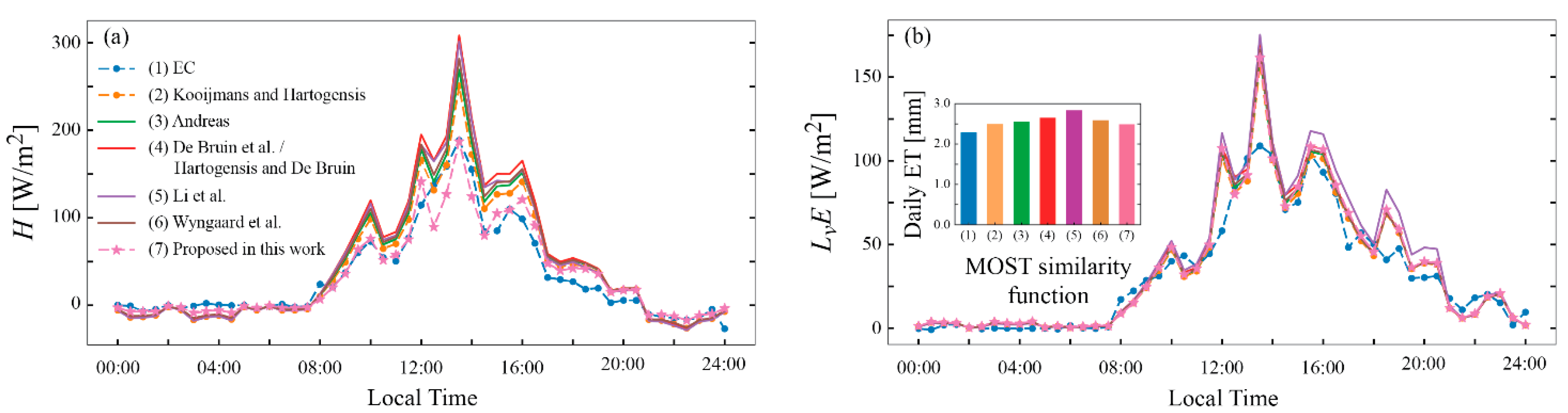
Although f C T 2 and f C q 2 are assumed to be universal, it has been shown that different MOST functions can cause an up to 20% difference in H estimations [35]. Wyngaard et al. [36] found general similarity functions for unstable (z/LO < 0) and stable (z/LO > 0) conditions:
f C x 2 u n s t a b l e ( z d L O ) = c x 1 ( 1 c x 2 z d L O ) 2 / 3
f C x 2 s t a b l e ( z d L O ) = c x 1 ( 1 + c x 2 ( z d L O ) 2 / 3 )
where x refers to T for temperature and q for humidity, and c x i are empirical coefficients. As shown in Table 1, there are many MOST functions in the scientific literature. Here, the Wyngaard et al. [36] formulation was selected, as they were used by de Bruin et al. [34] to assess scintillometry over a vineyard located in an arid region.
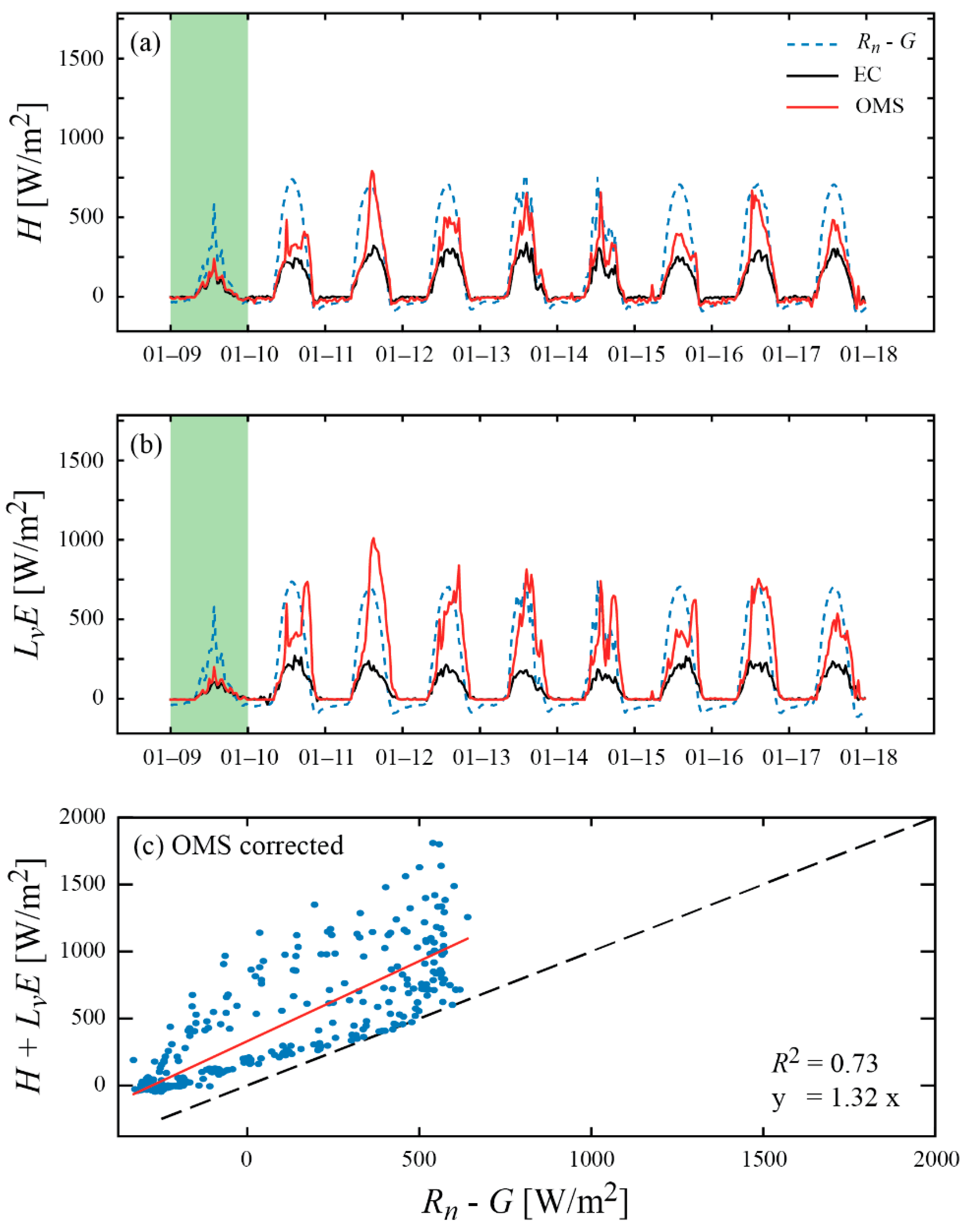
When using a standalone LAS, Bowen’s correction shown in Equation (5) allows calculation of H [W/m2] without making measurements or assumptions about humidity fluctuations [10]. However, LvE [W/m2] cannot be estimated directly, since C q 2 is disregarded. Thus, the surface EBC is typically used to obtain LvE after H has been estimated [39]:
R n G = H + L v E
where Rn is net radiation [W/m2], and G is the ground heat flux [W/m2]. As a convention, it is considered that Rn is positive when directed into the surface, while the other fluxes are positive when directed away from it. This method will be referred to as the standalone LAS method.

2.2. Study Area, Instrumentation, and Collected Data

The study area is an irrigated vineyard of 12 ha located in Pirque [40], an agriculture-based province located in the semi-arid Central valley of Chile surrounded by neighbouring land also used for agricultural activities or very dry wasteland (Figure 1a). Vineyards are north–south oriented in a vertical trellis system with a vegetation height of ~1.6 m, with little variations throughout the study site. The space between rows is 2.45 m and between plants is 1.20 m. This region has a semi-arid climate with typical annual rainfall amounts of about 460 mm and temperatures in summer ranging between 12–30.4 °C versus 4.4–14.3 °C in winter. Our field campaign was performed in the summer period between 9 January 2019 and 17 January 2019, where no precipitation and no changes in the grapes’ growth stage were observed. An EC system (IRGASON, Campbell Scientific Inc., Logan, UT, USA) and a meteorological station were set up in the middle of the vineyard 4 m above ground. The average wind speed observed over the vineyard was 1.5 m/s, with a maximum of 4.5 m/s and a minimum of 0.1 m/s. The highest wind speeds came mainly from the west (Figure 1a) over the afternoons. The 20-Hz EC data were processed to obtain 30-min fluxes using the EddyPro 6.2.2 software and activating the default recommended correction procedures [41,42]. The meteorological station included a temperature and relative humidity sensor (HMP45C, Campbell Scientific Inc., Logan, UT, USA), a net radiometer (NR Lite 2, Kipp & Zonen, Delft, The Netherlands), four soil heat flux plates (HFP01-L, Campbell Scientific Inc., Logan, UT, USA), two soil thermocouples (TCAV, Campbell Scientific Inc., Logan, UT, USA), and a water content reflectometer (CS616, Campbell Scientific Inc., Logan, UT, USA) All these sensors were connected to a datalogger (CR3000, Campbell Scientific Inc., Logan, UT, USA).
An OMS was installed at 3.02 m height in a NE–SW orientation over a 480-m path. The EC system and the meteorological station were located downwind near the center of the OMS path (Figure 1b). Under these conditions, the footprint of both systems covered the same type of vegetation and did not extend beyond the vineyard (see Appendix A). Therefore, the estimates of H and LvE from the EC and the OMS were comparable, and ET fluxes at the plot scale could be determined. The OMS was composed of a LAS (LAS MkII, Kipp & Zonen, Delft, The Netherlands), with an aperture of 149 mm and a wavelength of 850 nm, and an MWS (RPG-MWSC-160, RPG Radiometer Physics GmbH, Meckenheim, Germany), with an aperture of 300 mm and a wavelength of 1.86 mm. The zero-plane displacement height was 1.12 m, and the roughness caused by the crops was 0.2 m [43]. The zero-plane displacement height was estimated from the crop averaged height ( H v e g = 1.6   m ) as d = 0.7 H v e g [44]. 1 kHz raw scintillometer data were saved to perform the spectral cleaning method.
As shown in Figure 1, the vineyard is not completely homogeneous, as it has rows of plants and rows of bare soil. Nonetheless, considering the small horizontal scale of these heterogeneities and that the height of the plants is fairly constant, the experimental configuration of both the EC and OMS was believed to be at or above the blending height. The blending height is the elevation at which the turbulent signatures of each surface are mixed and above which MOST is generally accepted to be applicable [11]. Moreover, our study site resembled that of Ezzahar et al. [45], in which sensible and latent heat fluxes were successfully determined over olive trees. In their study, the ratio between the height of the trees and the instruments was 0.43, whereas in this study, this ratio was 0.53 for the OMS and 0.40 for the EC.

2.3. Data Quality Metrics

Orthogonal regressions were performed to quantify the EBC quality of the different methods assessed in this work. From the orthogonal regressions of the EBC, the slope and the determination coefficient (R2) of the best linear regression curve were determined. Furthermore, the energy balance ratio (EBR) was computed to analyze the EBC [15]:
EBR = H + L v E R n G
The EBR allows one to evaluate the EBC by summing H and LvE and RnG over specified time periods. The Nash–Sutcliffe efficiency (NSE) was estimated to analyze the method’s agreement and accuracy compared to EC measurements. Percentage values of overestimation or underestimation with respect to the EC system were also reported.

2.4. Spectral Cleaning of the Raw Signal Intensities

Unwanted contributions to the OMS intensity variances can result in unrealistic heat fluxes [22,46]. The proposed spectral data cleaning process is shown in Figure 2. The first step in this process is to identify unwanted contributions to the 1-kHz scintillometer raw signal by performing a spectral analysis. The spectral analysis allows one to detect absorption at low frequencies, erratic spikes and tripod vibrations [47,48] within the scintillometer frequencies, and electronic noise in high frequencies. The second step is to apply the electronic noise and absorption filter presented in Figure 2. To eliminate these unwanted contributions, Stoffer [18] recommends applying BPFs to the original spectrum: a 0.1 Hz high-pass filter (HPF) and a 100 Hz low-pass filter (LPF). Thus, any frequency contribution below 0.1 Hz or above 100 Hz is cut off from both LAS and MWS signals. Here, we applied Stoffer’s [18] BPFs and assessed the recovered signal variance to ensure that the signal contained only contributions from the scintillation properties related to the heat fluxes. Based on Clifford [49] scintillation spectra, the application of the 0.1-Hz HPF with a minimum cross wind of ~0.1 m/s recovers more than 90% of the signal variance for the LAS and more than 90% for the MWS. Based on Clifford [49] scintillation spectra, the application of the 0.1-Hz HPF with a minimum cross wind of ~0.1 m/s recovers more than 90% of the signal variance for the LAS and more than 90% for the MWS; whereas the 100-Hz LPF with a maximum cross wind of ~4 m/s recovers more than 99% of the LAS and MWS signal variances. Then, the third step is to apply a filtering process of erratic spikes and unwanted contributions from tripod vibrations. This step is not trivial, as typically, tripod vibration frequencies are within the scintillometer frequencies, which are relevant for computing heat fluxes. Therefore, it needs to be carried out carefully to avoid filtering the correct signal that should be used by the LAS and MWS. The method shown in Figure 2 consists in dividing the spectrum in blocks of 5% of the total data and calculating the block’s median (MED) and mean absolute deviation (MAD).
Then, erratic peaks and tripod vibrations within the data block are defined when the following condition is met:
S f > MED + a MAD             i f             f r e q u e n c y FT   Hz
S f > MED + b MAD             i f             f r e q u e n c y > F T   Hz
where Sf is the value of the spectrum in the frequency range, a and b are empirical coefficients, and FT [Hz] is a frequency threshold. Hence, the values of a and b should be defined for each dataset, as they depend on the unwanted contributions to the scintillometer signal that appear in the spectra. The FT also needs to be selected for each set of data (e.g., 2 Hz is generally where tripod vibrations occur). When the erratic peaks of one data block are found, the next block to be analyzed is overlapped to ensure continuity, and the process is repeated until the unwanted contributions of all the blocks are found. To remove the unwanted contributions of erratic peaks and tripod vibrations, their Fourier coefficients are randomly varied by assuming that they distribute uniformly within each data block, so the relevant statistical properties are not modified. As this approach could produce new artificial erratic peaks, an iterative process is carried out until all the unwanted contributions are removed.
Figure 3 shows an example of the spectral data cleaning method. In this example, a random spectrum is used (Figure 3a). A BPF removes absorption and electronic noise of the original spectrum. As a result, any frequency contributions below the HPF and above the LPF are removed (Figure 3b). Then, the spectrum is evaluated in blocks to identify unwanted contributions from tripod vibrations and erratic spikes. This process is performed from low to high frequencies (Figure 3c). As shown in Equations (15) and (16), the criteria to categorize an unwanted contribution will depend on the frequency threshold (FT). Thus, a corrected spectrum without electronic noise, absorption, erratic spikes, and unwanted contributions from tripod vibrations is obtained (Figure 3d).
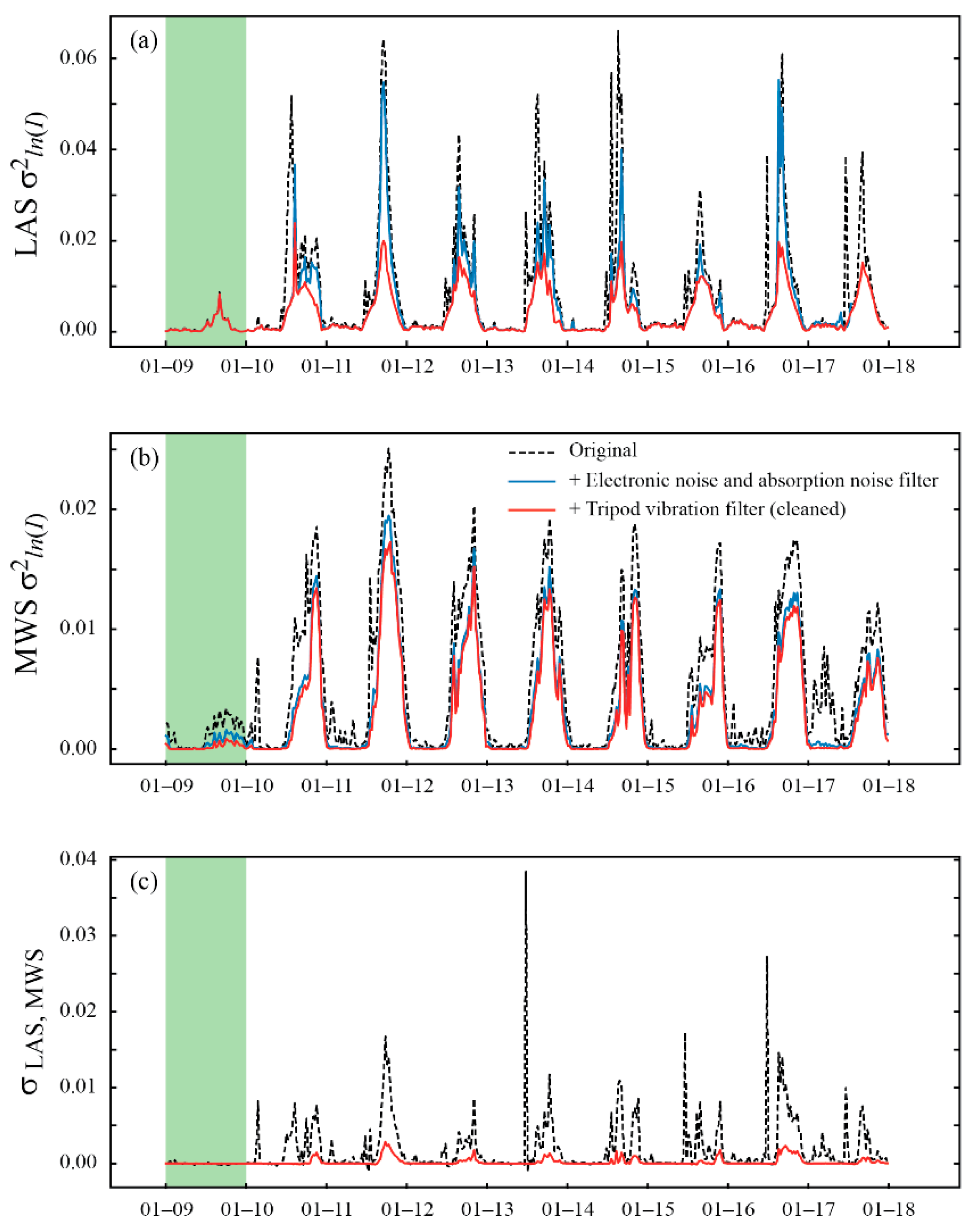
From the cleaned spectrum, the variance of the signal is calculated using the integral of the spectrum curve, as the spectrum is scaled such that the area under the spectrum is proportional to the signal variance. Furthermore, the corrected signal time series is estimated using the inverse fast Fourier transform (IFFT). The spectral cleaning method was performed using a time step of 30 min to obtain the clean variances and signals for computing the heat fluxes. The entire dataset (9 January 2019 and 17 January 2019) was considered with the aim of analyzing the proposed method effectiveness for removing unwanted contributions with statistical significance, for which the scintillometer heat fluxes are presented before and after the cleaning process using the Hill [16] method. In the results presented below, we used different dates for the analysis, depending on the quality of the collected data.

2.5. OMS Sensitivity to Selected C T 2 - C q 2 Methods and MOST Analysis

This section aims to compare the estimations of H and LvE based on the choice of the different theoretical methods assessed, i.e., the standalone LAS [15], the Hill [16] method, the Lüdi et al. [17], and the hybrid [18] methods, as well as on the choice of the MOST similarity functions. The day with the best-quality data (9 January 2019) was selected to compare the results to those obtained with EC.
The scintillometer theoretical method that best agreed with the EC measurements was chosen to perform the sensitivity analysis of the MOST similarity functions. For this analysis, the functions presented in Table 1 were used. Furthermore, new MOST similarity functions were proposed for the conditions observed in the vineyard by iterating c T 1 for obtaining H. Once the best agreement between H E C and H O M S was found, c q 2 was modified until finding the best agreement between L v E E C and L v E O M S .

3. Results

3.1. EC Fluxes and OMS Fluxes Prior to Spectral Cleaning

The H and LvE measured by the EC and OMS using the Hill [16] method to link C n 2 to C T 2 and C q 2 are presented in Figure 4. Both measuring systems show that flux partitioning was slightly tilted towards H, but H and LvE were roughly of the same magnitude throughout the campaign. The fluxes measured by the EC system were consistent with measurements performed in similar study sites with an EBR of 0.82 and energy balance correlation slope of 0.63 with R2 = 0.95. Even when the EC energy balance closure slope was relatively low (0.63), it was within values reported in other studies [11,13,50,51,52,53]. For instance, in a semi-arid area of China, the closure slope ranged between 0.52 and 0.90 [50], whereas values between 0.50 and 0.88 were reported in a semi-arid area of South Africa [51]. These imbalances are generally due to an overestimation of the available energy, measurement errors due to instrumentation or sampling problems, and soil and canopy heat storage [52,53]. For this reason, the EC imbalance reported in this study site is within an acceptable range. After 10 January 2019, the scintillometer fluxes were unrealistic, as (1) at specific times, the OMS-fluxes were much larger than the solar constant (~1360 W/m2 [46]); (2) the OMS-fluxes were much larger than the EC-based fluxes; (3) the OMS-fluxes were generally larger than the available energy (RnG); and (4) the large values of H and LvE resulted in an EBR of 2.95 and an energy balance correlation slope of 2.10, with R2 = 0.69 (Figure 4), which are extremely large values. Moreover, when comparing the original OMS fluxes with the EC measurements, an NSE’s of −6.59 and −23.34 were found for H and LvE, respectively, which indicate a bad OMS performance. Thus, Figure 4 suggests that an analysis of the raw scintillation data, average signal, and variances is needed to understand the unrealistic OMS heat fluxes magnitudes.
The averaged signal is a good indicator of the signal quality, since it is expected to be constant in time. Figure 5a shows an analysis of the averaged scintillometer signal intensity expressed as ln(I/Iavg). There were evident deviations from the average signal from 10 January 2019, which both increased and decreased, causing fluctuations around the signal mean value. These deviations occurred during the afternoons, coinciding with the hours where the study site presented elevated wind speeds (>2 m/s). Unstable tripods could have caused slight vibrations of the towers as a consequence of the wind, adding unwanted contributions to the signal. It also might have caused a temporal misalignment that could be seen from the average signal and from large variances shown in Figure 5b. This temporal misalignment between the scintillometers’ transmitter and receiver refers to the fact that the signal fluctuations measured by the receiver were captured on the edge of the equipment, because it was installed that way during the alignment process. Therefore, when high wind speeds reached the scintillometers, tripods vibrations caused an increase of the signal fluctuations as the light beam was constantly in and out of focus, overestimating the variances measured on the receiver and, consequently, the heat fluxes.
As shown in Figure 5a, the average signal deviated when wind speeds surpassed ~2 m/s. Therefore, wind flow possibly made the tripods vibrate due to their unstable condition. The original variances of the signals also presented the same behaviour (Figure 5b). From 10 January 2019, high variances were reached at the time when signal deviation due to elevated wind speeds occurred. Thus, average signal deviations and high signal variances were related. The largest signal deviation was detected during 10 January 2019. However, it coincided with an alignment process performed at 10:19 LT, where the field team manipulated the scintillometers. Note, also, that during nights, where wind speeds were low, OMS and EC measurements agreed (Figure 4).

3.2. OMS Results after Spectral Cleaning

3.2.1. OMS Spectra

A spectral analysis of the data using 30-min ranges was carried out to highlight the influence of unwanted contributions. Figure 6 presents two examples of the data obtained during the field campaign used to illustrate the filtering procedure (Figure 2 and Figure 3).
The first example is depicted in the left side of Figure 6. The raw 1 kHz LAS signal intensity, expressed as ln(I/Iavg), obtained on 10 January 2019 between 13:00 and 13:30 LT is shown in Figure 6a. Only the LAS signal is presented, as it was the signal most affected by the wind fluctuations. Figure 6b depicts the original spectrum related to the previous signal, where interesting features were observed. First, most of the energy was located between 1 and 50 Hz. Second, absorption fluctuations were occurring at frequencies lower than 0.1 Hz. Third, spectrum peaks at ~2 Hz suggest that tripod vibrations could have been occurring, as these typically have a natural frequency between 1 and 3 Hz [47,48]. Thus, the frequency threshold (FT) was defined as 2 Hz. The filtered spectrum where electronic noise and absorption were removed is presented in Figure 6c, in which the contributions from frequencies below 0.1 Hz and above 100 Hz were eliminated. The spectrum filtered with the approach proposed in this study is shown in Figure 6d, where the erratic peak at ~2 Hz, which was associated to tripod variations, was eliminated. However, the erratic spike and tripod vibrations filter created artificial peaks from the random process. Figure 6e shows the corrected LAS signal, in which the mean value remained constant. In this example, the erratic spike filtering process was not as important as the electronic noise filtering process.
The second example is presented in the right side of Figure 6. Figure 6f shows the original LAS signal, also expressed as ln(I/Iavg), obtained on 11 January 2019 between 17:30 and 18:00 LT. Figure 6g shows the original spectrum, where most of the energy was located between 2 and 7 Hz. For this case, the contribution from tripod vibrations was prominent, making the spectrum reach variances of 2.5. Spectrum peaks located between 2 and 3 Hz suggest again that tripod vibrations could be occurring. Unlike the previous example, the filtered spectrum without electronic noise and absorption (Figure 6h) did not show considerable differences with Figure 6g, as no contributions from frequencies below 0.1 Hz and above 100 Hz were detected. However, Figure 6i shows that the tripod vibrations’ filtering process had an impact on the spectrum, where the maximum values of the spectrum in the frequency range (i.e., the variances) were reduced from approximately 2.5 to 0.8 (note the change in scale of the vertical axis between Figure 6h,i). Figure 6j shows the corrected LAS signal, in which the mean value also remained constant, but less fluctuations around it were observed. In this example, unwanted contributions from tripod vibrations were more important than absorption from low frequencies. Thus, wind speed considerably affected scintillometer heat fluxes estimations by producing unwanted contributions from tripod vibrations but also by additional fluctuations due to misalignment.

3.2.2. OMS Variances and Fluxes

The variance and covariance of the LAS and MWS scintillometer signals were computed from the corrected signal as the area under the spectrum (Figure 7). This analysis helps to quantify how much of the unwanted contributions correspond to electronic noise and absorption and how much correspond to high wind speeds and bad alignments.
The spectral cleaning method reduced unwanted contributions, since signal variances (Figure 7a,b) and covariance (Figure 7c) after applying each filter reached lower values. However, the spectral cleaning method proposed in this work did not guarantee a complete signal cleaning, as there were still large values of the variances observed between 10 January 2019 and 17 January 2019. For instance, the erratic spike of σLAS2 during 10 January 2019, which occurred due to an alignment of the scintillometers, was still observed. Nonetheless, the signals were greatly improved. The LAS signal had more unwanted contributions than the MWS signal. On one hand, the erratic spikes and tripod vibrations filter reduced the variances more than the electronic noise and absorption filter (see LAS scintillation statistics in Figure 7a). On the other hand, electronic noise and absorption were more relevant for the MWS scintillation statistics (Figure 7b).
From the corrected variances, it was possible to recalculate OMS-based heat fluxes (Figure 8). Similarly, as the original OMS fluxes, the corrected heat fluxes were estimated using the Hill [16] method. Figure 8 and Table 2 show these fluxes and their comparison to the results obtained from the EC system. For the corrected fluxes, H and LvE represented 62.3 and 79.6% of daily total Rn, respectively, and the EBR was now 1.78. Even when the corrected heat fluxes had smaller magnitudes compared to the original fluxes, the cleaning process was not enough to improve the data after the misalignment occurred (10 January 2019), as the fluxes were still too large, and both the energy balance correlation slope (1.32, with R2 = 0.73) and NSE’s (NSEH = −0.12 and NSELvE = −6.63) still indicated an OMS bad performance (with the exception of those observed on 9 January 2019).

3.3. OMS Sensitivity to Selected C T 2 - C q 2 Methods and MOST Analysis

To isolate the effect of tripod vibrations on the OMS signal without having data influenced by the temporal misalignment, the effectiveness of the different theoretical methods and the MOST analysis was performed using the best-quality data obtained on 9 January 2019. Figure 9 presents the heat fluxes (left side) and energy balance closure (right side) obtained by the EC and estimated from the OMS original fluxes using the Hill [16] method and the corrected OMS fluxes using the four theoretical methods for 9 January 2019. Table 3 shows the heat fluxes as a percentage of Rn, as well as the EBR. Note that an EBR = 1.00 for the standalone LAS [15] method occurred, because LvE is derived as a residual of the energy balance.
The original H and LvE OMS fluxes for 9 January 2019 were 46.2 and 76.3% of the daily total Rn, and the EBR was estimated as 1.52 (Table 3). The daily ET was found to be 6.07 mm. For the corrected OMS fluxes using the same approach (the Hill [16] method), the results were more reasonable, as H and LvE were 45.2 and 38.1% of the daily total Rn, the EBR was 0.98, and a daily ET was found to be 3.07 mm. Thus, for 9 January 2019, the spectral cleaning process significantly reduced the LvE, and the corrected H + LvE never surpassed RnG. The EC system measurements for 9 January 2019 showed that H and LvE represented 33.8 and 28.9% of the daily total Rn, respectively, with an EBR of 0.79, and the total daily ET was 2.29 mm. Therefore, the corrected OMS heat fluxes agreed much better with the EC results.
To analyze the performance of the different theoretical methods, scatter plots comparing the EC and corrected OMS fluxes are shown in Figure 10. Table 4 summarizes the OMS overestimations and underestimations when comparing the results to those obtained with the EC system, while correlation slopes, determination coefficients, and NSE’s are presented in Table 5.
For all methods, scintillometer measurements estimated larger values of H in comparison with EC results (Table 4). During the night, scintillometer methods estimated larger negative values than EC, while during the day, they estimated larger positive values than EC. When H was larger than 100 W/m2, a larger scatter was observed. However, all methods showed a great performance for estimating H, with a correlation slope of 1.2, R2 = 0.96, and NSE = 0.91 (Table 5). If H quantification was needed, the Hill [16] method yielded similar results to those obtained by the EC system.
For LvE, a greater disagreement between the scintillometer and EC method was observed, compared to the H results. This was especially true for the standalone LAS [15] method, which overestimated LvE from the EC method by 101% (Table 4), with a correlation slope of 2.08, a determination coefficient of 0.809, and an NSE coefficient of 0.574 (Table 5). This result indicated a much worse performance of the standalone LAS [15] method compared to the other methods for estimating LvE, as from the correlation slope, it is clear that it doubled the ECLvE value. The issue with the standalone LAS [15] method was expected, since the EC system showed an energy imbalance with an EBR of 0.79, and the standalone LAS [15] method estimated LvE as the residual in the energy balance closure. Regarding the other three methods, they all had the same determination coefficient (0.914; Table 5), and all of them estimated higher values for LvE compared to EC during the day. These three scintillometer methods yielded very similar results to those obtained by EC, with the Lüdi et al. [17] method being the closest to EC (overestimation of 14% of LvE, as shown in Table 4). Furthermore, the Lüdi et al. [17] method presented a correlation slope of 1.07 and a NSE coefficient of 0.904 when compared to EC (Table 5).
The heat fluxes obtained with different MOST similarity functions are presented in Figure 11. These fluxes were estimated with the Lüdi et al. [17] method, as this approach better resembled the EC results (see Figure 9, Table 5 and Table 6). The MOST similarity functions proposed coefficients for cT1 and cT2 in the field campaign that were 5.5 and 15.1 and 5.6 and 1.9 for stable and unstable conditions, respectively. The proposed cq1 and cq2 coefficients were 4.5 and 1.1 and 4.5 and 9.9 for stable and unstable conditions, respectively. Table 6 shows how much the different similarity functions applied in the Lüdi et al. [17] method overestimated (+) or underestimated (-) the heat fluxes compared to the EC measurements, and it compares these to the fluxes obtained when the Kooijmans and Hartogensis [21] MOST similarity functions are used. NSE’s compared to the EC system are also included. As shown in Table 6, the MOST similarity functions proposed by Kooijmans and Hartogensis [21] were the ones that worked better for describing the conditions observed in the vineyard (NSEH = 0.91 and NSELvE = 0.90). As expected, the MOST similarity functions proposed in this research agreed better with EC measurements (NSEH = 0.92 and NSELvE = 0.91), as this was the main aim of developing them.

4. Discussion

Scintillometer-based heat fluxes can be strongly altered when wind currents affect the measurement’s physical setup. In this work, the unrealistic heat fluxes, obtained prior to reprocessing the scintillometer data, were mostly due to deviations on the average signal produced when wind caused tripod vibration. As our spectral analysis showed unwanted contributions at different frequencies, a spectral filtering method was used to remove unwanted contributions due to electronic noise, absorption, and erratic spikes, and it was extended to remove the effect of tripod vibrations, which was the novelty of this work. Removing tripod vibrations fluctuations has not been widely addressed before, as removing unwanted contributions from in between the optical and microwave frequencies used by scintillometers to estimate H and LvE is challenging. However, they can easily double the magnitude of σln2(I), strongly influencing the resulting heat fluxes. Even when the spectral data cleaning method proposed in this work will not always be perfect, as it uses a probabilistic approach to remove unwanted contributions to the scintillometer signal, the corrected variances were more realistic (Figure 7) after filtering the data, and the corrected H and LvE agreed much better with the results obtained by the EC system (see Figure 4 and Figure 8).
In addition to performing the spectral cleaning of the raw data to remove unwanted contributions to the signal, our analysis showed that to estimate the scintillometer-based heat fluxes, it was important to analyze which theoretical method and MOST similarity function were best suited for each field campaign. As most of the previous investigations available in the scientific literature deal with H measurements [34,54,55,56], this analysis was crucial when estimating LvE (and, consequently, ET).
On one hand, the four theoretical methods evaluated in this work agreed fairly well with the sensible heat measured by the EC system (HEC), with the Hill [16] method achieving the best results (Figure 10a). The R2 values related to H were higher than 0.95, the NSE’s were 0.91 for all the methods, and the correlation slope between the scintillometer-based H and the HEC were between 1.20 and 1.24 (Table 5). These metrics agree with results presented in the literature [10,16,39,40,41]. On the other hand, the selection of the method for scintillometer-based LvE (ET) estimations can lead to considerable differences. As shown in Figure 10b, the LvE estimated using scintillometer methods showed more dispersion when compared to LvE measured by the EC system (LvEEC), with the Lüdi [17] method and the standalone LAS [15] methods providing the best and worst results, respectively. Note that a worse performance of the standalone LAS method [15] was expected, since using only a LAS to compute LvE will always lead to errors when significant energy imbalances are present. The R2 values related to LvE were 0.91 for all the methods, and the correlation slope and NSE coefficient between the scintillometer-based LvE and LvEEC were between 1.07–1.38 and 0.79–0.9, respectively, with the exception of the standalone LAS method, which reported values of R2 = 0.81 and NSE = 0.57 (Table 5). Few studies comparing OMS and EC results exist in the scientific literature. Meijninger et al. [19] investigated OMS measurements over a heterogeneous terrain that consisted of forests (43%), agricultural fields and meadows (45%), lakes (7%), and small built-up areas (5%) in a cool temperate climate region. They installed their scintillometers above the blending height and found an R2 of 0.87 between LvE estimates obtained with an OMS and an EC, with a correlation slope of 1.26. Yee et al. [13] measured heat fluxes in an arid region dominated by perennial tussock grasses, and they found poor agreement for LvE, with correlation slopes ranging between 3.19 and 4.44 compared to LvEEC.
Understanding the factors that lead to differences between OMS and EC measurements is important. First, there is a footprint difference, as scintillometers usually cover larger areas than an EC [56]. Second, EC systems cannot capture energy fluxes from larger eddies or from secondary circulations that do not touch the ground or that are stationary over the same terrain structures that generate them, i.e., bypassing the EC system [52,56]. Thus, methods that use spatial averaging, such as scintillometers, may exhibit a tendency to better close the energy balance, which was observed in the present research (Table 3). Third, uncertainties related to the input variables of scintillometer methods can affect the resulting scintillometer-based heat fluxes. These uncertainties depend on the spatial variation of the input variables along the scintillometer path, as well as on systematic error. According to Hartogensis et al. [35] and Yee et al. [13], the input variable that has a great impact on the results is the effective height. Therefore, care must be taken when measuring the vertical distance between the light beam and the surface in which the measurements are being carried out.
Moreover, the different scintillometer theoretical methods also cause discrepancies between the estimated surface heat fluxes. These differences can be related to r T q , which can lead to inaccurate assignment of the structure parameters of temperature and humidity [13,17,57]. For instance, using precise r T q values allowed Lüdi et al. [17] to reach an average reduction of 13% on C q 2 , implying that LvE fluxes were overestimated when assuming perfect correlation. Furthermore, Wesely [30] and Leijnse et al. [58] demonstrated that uncertain values for r T q can cause larger errors in flux estimates for dry conditions, which was also reported by Yee et al. [13] and Alfieri et al. [59]. For our study site, the exact computed value of r T q did not result in significant changes in the H estimation. However, this was not the case when estimating LvE, where the large differences in LvE occurred when the sign of r T q differed between methods during daytime. Meijninger et al. [19] explains that C q 2 is more sensitive than C T 2 due to a non-local effect when the fluctuations of T and q are not correlated; hence, r T q measurements have an important impact on C q 2 (and, therefore, on LvE), whereas C T 2 shows no considerable response to r T q values. Thus, understanding the r T q behaviour is complicated. As r T q indicates the correlation between T and q fluctuations, it does not directly specify the sign of H and LvE; rather, it specifies the sign of the Bowen ratio. Thus, an additional assumption to estimate heat fluxes is needed for the scintillometer theory. Generally, LvE is assumed to be always positive, and H defines the sign of r T q . Despite this, sometimes when there is mist or dew on the surface given by water vapor in the atmosphere at night, LvE can be slightly negative (although very close to zero). This highlights the importance of performing a spectral cleaning before obtaining the meteorological structure parameters and r T q that will be used to determine scintillometer-based H and LvE.
MOST functions can also explain differences between the EC and OMS measurements. In this study, the similarity functions reported by Kooijmans and Hartogensis [21] for estimating H and LvE resulted in a good agreement between EC and OMS measurements (NSEH = 0.91 and NSELvE = 0.9). However, the different similarity functions used to determine LvE resulted in differences of ±12% between the two methods. Scintillometer-based estimations were improved by proposing new coefficients, which were based on the Kooijmans and Hartogensis [21] MOST similarity functions. Note that the larger sensitivity of C q 2 compared to C T 2 described by Meijninger et al. [19] can also be inferred by the large variability of the parameters that define the MOST similarity functions (see Table 1). Hence, similarity functions can yield inaccuracies, especially for LvE (and ET) quantification. In the absence of MOST similarity functions developed for a specific site, the authors recommend using the functions developed by Kooijmans and Hartogensis [21], as they are based on 11 field campaigns and have higher probabilities to function better in any study area. Finally, it is important to note that the analysis of the different MOST similarity functions was performed with one day of data. Therefore, more data should be collected and analyzed to strengthen our conclusions.

5. Conclusions

This investigation demonstrated that tripod vibrations that might be caused by high wind speed can strongly increase scintillometer-based heat fluxes, to the point of reaching unrealistic values of H and LvE (and, consequently, ET). A high wind speed can alter scintillometer data through (1) tripod vibrations, (2) misalignments due to LAS and MWS movement, and (3) electronic noise and absorption contributions to the signal. Therefore, reprocessing scintillometer data through the spectral analysis proposed in this work is an important step for computing scintillometer-based heat fluxes. Therefore, future researchers who face partially damaged scintillometer signals can resort to this method and recover the data through the cleaning method proposed in this research by evaluating the signal spectrum and determining the a, b, and FT parameters from the spectral data cleaning method for their own dataset.
This research also found that the selection of the scintillometer theoretical method and the MOST similarity functions affected the resulting heat fluxes. On one hand, it was found that H estimations were less sensitive to the selection of the theoretical method, compared to the LvE (and ET) estimations. The LvE estimates were sensitive to how r T q was calculated, which explained the larger variability observed in these estimates. The Lüdi method LvE estimates were closer to those obtained with the EC system, overestimating them in 14%, with a correlation slope of 1.07, a coefficient of determination of 0.91, and an NSE of 0.90. On the other hand, differences of ±12% in LvE were found when using different MOST similarity functions. Our results show that the Kooijmans and Hartogensis [21] functions were accurate for describing the vineyard at our study site, as they were developed using data from 11 different field campaigns. Nonetheless, new proposed similarity functions yielded better results for the vineyard in Pirque, as they were site-specific. Thus, it appears that the MOST coefficients found in this research can be used in other studies where meteorological conditions and the terrain are similar to the present case. However, in general, it is recommended to adjust coefficients specific to the study site.
As the scintillometer-based ET fluxes strongly depend on the quality of the raw data, it is strongly recommended to apply the spectral cleaning method, as it greatly improves scintillometer data. Furthermore, it is important to understand the limitations and differences between the different theoretical methods and similarity functions used by scintillometry, as their selection has an impact on r T q values and, thus, on LvE, which is relevant when quantifying ET through the scintillometer theory.

Author Contributions

Conceptualization and methodology, O.H., F.A., F.M. and F.S.; validation and formal analysis, F.A.; writing—original draft preparation, F.A., O.H., F.M. and F.S.; writing—review and editing, F.A., O.H. and F.S.; supervision, O.H. and F.S.; project administration and funding acquisition, F.M. and F.S. All authors have read and agreed to the published version of the manuscript.

Funding

This research and the APC were funded by the Agencia Nacional de Investigación y Desarrollo (ANID), by grants ANID/FONDECYT/1210221, ANID/FONDECYT/1170429, and ANID/FONDEQUIP/EQM170024.

Data Availability Statement

The data used in this work can be requested by email to the corresponding author.

Acknowledgments

The authors thank the Centro de Desarrollo Urbano Sustentable (CEDEUS–ANID/FONDAP/15110020) and the Centro de Excelencia en Geotermia de los Andes (CEGA–ANID/FONDAP/15200001) for supporting this investigation. F.A. acknowledges the financial support of ANID by Beca Doctorado Nacional 2021-21211730 Furthermore, the authors acknowledge field support from A. Luque, V. García, F. Medel, M. Lillo, M. Signorio, M. Mendoza, M.C. Muñoz, and J. Araya. We also thank the feedback provided by two anonymous reviewers and the academic editor, which greatly improved the presentation of this work.

Conflicts of Interest

The authors declare no conflict of interest and declare that the funders had no role in the design of the study; in the collection, analyses, or interpretation of data; in the writing of the manuscript, or in the decision to publish the results.

Abbreviations

Acronyms
BPFBand pass filter
EBCEnergy balance closure
EBREnergy balance ratio
ECEddy covariance
ETEvapotranspiration
FTFrequency threshold
HPFHigh pass filter
IFFTInverse Fourier fast transform
LASLarge aperture scintillometer
LPFLow pass filter
MADMean absolute deviation
MEDMedian
MOSTMonin-Obukhov similarity theory
MWSMicrowave scintillometer
NSENash-Sutcliffe efficiency
OMSOptical microwave scintillometer
Variables and constants
σ2ln(I)Signal intensity variance
C n 2 Refractive index structure parameter
C q 2 Specific humidity structure parameter
C T 2 Temperature structure parameter
C T q Temperature-humidity correlation structure parameter
HSensible heat flux
LvELatent heat flux
RnNet radiation
GGround heat flux
loptOptical range wavelength
lmwMicrowave range wavelength
copt, cmw & copt,mwConstants for optical, microwave and optical-microwave
LPath length
DOptical scintillometer diameter
FFresnel length
TTemperature
QSpecific humidity
AiDimensionless coefficients
cpSpecific heat at constant pressure
βBowen ratio
r T q Temperature-humidity correlation
rAir density
u*Friction velocity
zBeam effective height
dZero-plane displacement
f C x 2 MOST universal similarity functions
LOObukhov length
κvon Kármán constant
T*Scaling temperature
SfValue of the spectrum in a frequency range
R2Coefficient of determination

Appendix A. Footprint Analysis

Figure A1 demonstrates that the footprint of the EC and the OMS systems covered the same type of vegetation and did not extend beyond the vineyard.
Figure A1. Footprint generated using data under unstable atmospheric conditions on 9 January at 16:00 using the Kljun et al. [23] method.
Water 14 00474 g0a1

References

  1. Lemeur, R.; Zhang, L. Evaluation of Three Evapotranspiration Models in Terms of Their Applicability for an Arid Region. J. Hydrol. 1990, 114, 395–411. [Google Scholar] [CrossRef]
  2. Parasuraman, K.; Elshorbagy, A.; Carey, S.K. Modelling the Dynamics of the Evapotranspiration Process Using Genetic Programming. Hydrol. Sci. J. 2007, 52, 563–578. [Google Scholar] [CrossRef]
  3. Ryken, A.C.; Gochis, D.; Maxwell, R.M. Unraveling Groundwater Contributions to Evapotranspiration and constraining water fluxes in a High-Elevation Catchment. Hydrol. Processes 2022, 36, e14449. [Google Scholar] [CrossRef]
  4. Figuerola, P.I.; Berliner, P.R. Evapotranspiration under Advective Conditions. Int. J. Biometeorol. 2005, 49, 403–416. [Google Scholar] [CrossRef]
  5. Mohawesh, O.E. Evaluation of Evapotranspiration Models for Estimating Daily Reference Evapotranspiration in Arid and Semiarid Environments. Plant Soil Environ. 2011, 57, 145–152. [Google Scholar] [CrossRef] [Green Version]
  6. Zhang, B.; Kang, S.; Li, F.; Zhang, L. Comparison of Three Evapotranspiration Models to Bowen Ratio-Energy Balance Method for a Vineyard in an Arid Desert Region of Northwest China. Agric. For. Meteorol. 2008, 148, 1629–1640. [Google Scholar] [CrossRef]
  7. Li, S.; Kang, S.; Zhang, L.; Zhang, J.; Du, T.; Tong, L.; Ding, R. Evaluation of Six Potential Evapotranspiration Models for Estimating Crop Potential and Actual Evapotranspiration in Arid Regions. J. Hydrol. 2016, 543, 450–461. [Google Scholar] [CrossRef]
  8. Wilson, K.B.; Hanson, P.J.; Mulholland, P.J.; Baldocchi, D.D.; Wullschleger, S.D. A Comparison of Methods for Determining Forest Evapotranspiration and Its Components: Sap-Flow, Soil Water Budget, Eddy Covariance and Catchment Water Balance. Agric. For. Meteorol. 2001, 106, 153–168. [Google Scholar] [CrossRef]
  9. Mobilia, M.; Longobardi, A. Prediction of Potential and Actual Evapotranspiration Fluxes Using Six Meteorological Data-Based Approaches for a Range of Climate and Land Cover Types. ISPRS Int. J. Geo-Inf. 2021, 10, 192. [Google Scholar] [CrossRef]
  10. Liu, S.M.; Xu, Z.W.; Zhu, Z.L.; Jia, Z.Z.; Zhu, M.J. Measurements of Evapotranspiration from Eddy-Covariance Systems and Large Aperture Scintillometers in the Hai River Basin, China. J. Hydrol. 2013, 487, 24–38. [Google Scholar] [CrossRef]
  11. Meijninger, W.M.L.; Green, A.E.; Hartogensis, O.K.; Kohsiek, W.; Hoedjes, J.C.B.; Zuurbier, R.M.; De Bruin, H.A.R. Determination of Area-Averaged Water Vapour Fluxes with Large Aperture and Radio Wave Scintillometers over a Heterogeneous Surface—Flevoland Field Experiment. Bound.-Layer Meteorol. 2002, 105, 63–83. [Google Scholar] [CrossRef]
  12. Van Kesteren, B.; Hartogensis, O.K.; van Dinther, D.; Moene, A.F.; De Bruin, H.A.R. Measuring H2O and CO2 Fluxes at Field Scales with Scintillometry: Part I—Introduction and Validation of Four Methods. Agric. For. Meteorol. 2013, 178–179, 75–87. [Google Scholar] [CrossRef]
  13. Yee, M.S.; Pauwels, V.R.N.; Daly, E.; Beringer, J.; Rüdiger, C.; McCabe, M.F.; Walker, J.P. A Comparison of Optical and Microwave Scintillometers with Eddy Covariance Derived Surface Heat Fluxes. Agric. For. Meteorol. 2015, 213, 226–239. [Google Scholar] [CrossRef]
  14. Monin, A.S.; Obukhov, A.M. Basic Laws of Turbulent Mixing in the Surface Layer of the Atmosphere. Contrib. Geophys. Inst. Acad. Sci. USSR 1954, 24, 163–187. [Google Scholar]
  15. Ezzahar, J.; Chehbouni, A.; Er-Raki, S.; Hanich, L. Combining a Large Aperture Scintillometer and Estimates of Available Energy to Derive Evapotranspiration over Several Agricultural Fields in a Semi-Arid Region. Plant Biosyst. Int. J. Deal. All Asp. Plant Biol. 2009, 143, 209–221. [Google Scholar] [CrossRef] [Green Version]
  16. Hill, R.J. Algorithms for Obtaining Atmospheric Surface-Layer Fluxes from Scintillation Measurements. J. Atmos. Ocean. Technol. 1997, 14, 456–467. [Google Scholar] [CrossRef]
  17. Lüdi, A.; Beyrich, F.; Mätzler, C. Determination of the Turbulent Temperature–Humidity Correlation from Scintillometric Measurements. Bound.-Layer Meteorol. 2005, 117, 525–550. [Google Scholar] [CrossRef] [Green Version]
  18. Stoffer, R. Revisiting Raw Data Processing of Combined Optical-Microwave Scintillometers. Master’s Thesis, Wageningen University & Research, Wageningen, The Netherlands, 2018. [Google Scholar]
  19. Meijninger, W.M.L.; Beyrich, F.; Lüdi, A.; Kohsiek, W.; De Bruin, H.A.R. Scintillometer-Based Turbulent Fluxes of Sensible and Latent Heat Over a Heterogeneous Land Surface—A Contribution to Litfass-2003. Bound.-Layer Meteorol. 2006, 121, 89–110. [Google Scholar] [CrossRef]
  20. Van Dinther, D.; Hartogensis, O.K.; Moene, A.F. Crosswinds from a Single-Aperture Scintillometer Using Spectral Techniques. J. Atmos. Ocean. Technol. 2013, 30, 3–21. [Google Scholar] [CrossRef]
  21. Kooijmans, L.M.J.; Hartogensis, O.K. Surface-Layer Similarity Functions for Dissipation Rate and Structure Parameters of Temperature and Humidity Based on Eleven Field Experiments. Bound.-Layer Meteorol. 2016, 160, 501–527. [Google Scholar] [CrossRef] [Green Version]
  22. Von Randow, C.; Kruijt, B.; Holtslag, A.A.M.; de Oliveira, M.B.L. Exploring Eddy-Covariance and Large-Aperture Scintillometer Measurements in an Amazonian Rain Forest. Agric. For. Meteorol. 2008, 148, 680–690. [Google Scholar] [CrossRef]
  23. Kljun, N.; Calanca, P.; Rotach, M.W.; Schmid, H.P. A Simple Two-Dimensional Parameterisation for Flux Footprint Prediction (FFP). Geosci. Model Dev. 2015, 8, 3695–3713. [Google Scholar] [CrossRef] [Green Version]
  24. Van Kesteren, B. Measuring Water-Vapour and Carbon-Dioxide Fluxes at Field Scales with Scintillometry. Ph.D. Thesis, Wageningen University & Research, Wageningen, The Netherlands, 2012. [Google Scholar]
  25. Hill, R.J. Implications of Monin–Obukhov Similarity Theory for Scalar Quantities. J. Atmos. Sci. 1989, 46, 2236–2244. [Google Scholar] [CrossRef] [Green Version]
  26. Li, D.; Bou-Zeid, E.; De Bruin, H.A.R. Monin–Obukhov Similarity Functions for the Structure Parameters of Temperature and Humidity. Bound.-Layer Meteorol. 2012, 145, 45–67. [Google Scholar] [CrossRef]
  27. Wang, T.; Ochs, G.R.; Clifford, S.F. A Saturation-Resistant Optical Scintillometer to Measure Cn2†. J. Opt. Soc. Am. 1978, 68, 334–338. [Google Scholar] [CrossRef]
  28. Green, A.E.; Astill, M.S.; McAneney, K.J.; Nieveen, J.P. Path-Averaged Surface Fluxes Determined from Infrared and Microwave Scintillometers. Agric. For. Meteorol. 2001, 109, 233–247. [Google Scholar] [CrossRef]
  29. Moene, A.F. Effects of Water Vapour on the Structure Parameter of the Refractive Index for Near-Infrared Radiation. Bound. Layer Meteorol. 2003, 107, 635–653. [Google Scholar] [CrossRef]
  30. Wesely, M.L. The Combined Effect of Temperature and Humidity Fluctuations on Refractive Index. J. Appl. Meteorol. Climatol. 1976, 15, 43–49. [Google Scholar] [CrossRef]
  31. Andreas, E.L. Estimating Cn2 over Snow and Sea Ice from Meteorological Data. J. Opt. Soc. Am. A 1988, 5, 481–495. [Google Scholar] [CrossRef] [Green Version]
  32. Kohsiek, W.; Herben, M.H.A.J. Evaporation Derived from Optical and Radio-Wave Scintillation. Appl. Opt. AO 1983, 22, 2566–2570. [Google Scholar] [CrossRef]
  33. Stull, R. An Introduction to Boundary Layer Meteorology. Available online: https://www.springer.com/gp/book/9789027727688 (accessed on 1 December 2019).
  34. De Bruin, H.A.R.; Van Den Hurk, B.J.J.M.; Kohsiek, W. The Scintillation Method Tested over a Dry Vineyard Area. Bound. Layer Meteorol. 1995, 76, 25–40. [Google Scholar] [CrossRef]
  35. Hartogensis, O.K.; Watts, C.J.; Rodriguez, J.-C.; Bruin, H.A.R.D. Derivation of an Effective Height for Scintillometers: La Poza Experiment in Northwest Mexico. J. Hydrometeorol. 2003, 4, 915–928. [Google Scholar] [CrossRef]
  36. Wyngaard, J.C.; Izumi, Y.; Collins, S.A. Behavior of the Refractive-Index-Structure Parameter near the Ground. J. Opt. Soc. Am. JOSA 1971, 61, 1646–1650. [Google Scholar] [CrossRef]
  37. De Bruin, H.A.R.; Kohsiek, W.; Van Den Hurk, B.J.J.M. A Verification of Some Methods to Determine the Fluxes of Momentum, Sensible Heat, and Water Vapour Using Standard Deviation and Structure Parameter of Scalar Meteorological Quantities. Bound.-Layer Meteorol. 1993, 63, 231–257. [Google Scholar] [CrossRef]
  38. Hartogensis, O.; De Bruin, H.A.R. Monin–Obukhov Similarity Functions of the Structure Parameter of Temperature and Turbulent Kinetic Energy Dissipation Rate in the Stable Boundary Layer. Bound.-Layer Meteorol. 2005, 116, 253–276. [Google Scholar] [CrossRef]
  39. Culf, A.D.; Foken, T.; Gash, J.H.C. The Energy Balance Closure Problem. In Vegetation, Water, Humans and the Climate: A New Perspective on an Interactive System; Kabat, P., Claussen, M., Dirmeyer, P.A., Gash, J.H.C., de Guenni, L.B., Meybeck, M., Pielke, R.A., Eds.; Global Change—The IGBP Series; Springer: Berlin/Heidelberg, Germany, 2004; pp. 159–166. ISBN 978-3-642-18948-7. [Google Scholar]
  40. Tosoni, D.E.; Meza, F.J.; Lacy, S.N. Independent Estimation of Sensible and Latent Fluxes in a Vineyard Using Improved Surface Renewal Analysis. Appl Clim. 2021, 144, 1375–1385. [Google Scholar] [CrossRef]
  41. Fratini, G.; Mauder, M. Towards a Consistent Eddy-Covariance Processing: An Intercomparison of EddyPro and TK3. Atmos. Meas. Tech. 2014, 7, 2273–2281. [Google Scholar] [CrossRef] [Green Version]
  42. Suárez, F.; Lobos, F.; de la Fuente, A.; Vilà-Guerau de Arellano, J.; Prieto, A.; Meruane, C.; Hartogensis, O. E-DATA: A Comprehensive Field Campaign to Investigate Evaporation Enhanced by Advection in the Hyper-Arid Altiplano. Water 2020, 12, 745. [Google Scholar] [CrossRef] [Green Version]
  43. Hansen, F.V. Surface Roughness Lengths; U.S. ARmy Research Laboratory: White Sands Missile Range, NM, USA, 1993. [Google Scholar]
  44. Grimmond, C.S.B.; Oke, T.R. Aerodynamic Properties of Urban Areas Derived from Analysis of Surface Form. J. Appl. Meteorol. Climatol. 1999, 38, 1262–1292. [Google Scholar] [CrossRef]
  45. Ezzahar, J.; Chehbouni, A.; Hoedjes, J.C.B.; Chehbouni, A.H. On the Application of Scintillometry over Heterogeneous Grids. J. Hydrol. 2007, 334, 493–501. [Google Scholar] [CrossRef] [Green Version]
  46. Li, K.J.; Feng, W.; Xu, J.C.; Gao, P.X.; Yang, L.H.; Liang, H.F.; Zhan, L.S. Why Is the Solar Constant Not a Constant? ApJ 2012, 747, 135. [Google Scholar] [CrossRef] [Green Version]
  47. Pezo, M.L.; Bakić, V.V.; Marković, Z.J. Structural Analysis of Guyed Mast Exposed to Wind Action. Therm. Sci. 2016, 20, 1473–1483. [Google Scholar] [CrossRef]
  48. Ghafari, M.O.; McClure, G.; Zhang, X.H.; Gagnon, D. Assessing the Variability of Seismic Response Analysis of Tall Guyed Telecommunication Tower with Ambient Vibration Measurement; 15th World Conference on Earthquake Engineering: Lisbon, Portugal, 2012. [Google Scholar]
  49. Clifford, S.F. Temporal-Frequency Spectra for a Spherical Wave Propagating through Atmospheric Turbulence. J. Opt. Soc. Am. 1971, 61, 1285–1292. [Google Scholar] [CrossRef]
  50. Liang, J.; Zhang, L.; Cao, X.; Wen, J.; Wang, J.; Wang, G. Energy Balance in the Semiarid Area of the Loess Plateau, China. J. Geophys. Res. Atmos. 2017, 122, 2155–2168. [Google Scholar] [CrossRef]
  51. Majozi, N.P.; Mannaerts, C.M.; Ramoelo, A.; Mathieu, R.; Nickless, A.; Verhoef, W. Analysing Surface Energy Balance Closure and Partitioning over a Semi-Arid Savanna FLUXNET Site in Skukuza, Kruger National Park, South Africa. Hydrol. Earth Syst. Sci. 2017, 21, 3401–3415. [Google Scholar] [CrossRef] [Green Version]
  52. Wilson, K.; Goldstein, A.; Falge, E.; Aubinet, M.; Baldocchi, D.; Berbigier, P.; Bernhofer, C.; Ceulemans, R.; Dolman, H.; Field, C.; et al. Energy Balance Closure at FLUXNET Sites. Agric. For. Meteorol. 2002, 113, 223–243. [Google Scholar] [CrossRef] [Green Version]
  53. Rahman, M.M.; Zhang, W.; Wang, K. Assessment on Surface Energy Imbalance and Energy Partitioning Using Ground and Satellite Data over a Semi-Arid Agricultural Region in North China. Agric. Water Manag. 2019, 213, 245–259. [Google Scholar] [CrossRef]
  54. Zeweldi, D.A.; Gebremichael, M.; Wang, J.; Sammis, T.; Kleissl, J.; Miller, D. Intercomparison of Sensible Heat Flux from Large Aperture Scintillometer and Eddy Covariance Methods: Field Experiment over a Homogeneous Semi-Arid Region. Bound.-Layer Meteorol. 2010, 135, 151–159. [Google Scholar] [CrossRef] [Green Version]
  55. Xu, Z.; Liu, S.; Li, X.; Shi, S.; Wang, J.; Zhu, Z.; Xu, T.; Wang, W.; Ma, M. Intercomparison of Surface Energy Flux Measurement Systems Used during the HiWATER-MUSOEXE. J. Geophys. Res. Atmos. 2013, 118, 13,140–13,157. [Google Scholar] [CrossRef]
  56. Foken, T.; Mauder, M.; Liebethal, C.; Wimmer, F.; Beyrich, F.; Leps, J.-P.; Raasch, S.; DeBruin, H.A.R.; Meijninger, W.M.L.; Bange, J. Energy Balance Closure for the LITFASS-2003 Experiment. Appl Clim. 2010, 101, 149–160. [Google Scholar] [CrossRef]
  57. Evans, J.; McNeil, D.; Finch, J.; Murray, T.; Harding, R.; Verhoef, A. Evaporation Measurements at Kilometre Scales Determined Using Two-Wavelength Scintillometry. In Role of Hydrology in Managing Consequences of a Changing Global Environment: BHS Third International Symposium, 19–23 July 2010, Newcastle University, Newcastle upon Tyne, United Kingdom: London, United Kingdom; British Hydrological Society: London, UK, 2010; pp. 19–23. [Google Scholar]
  58. Leijnse, H.; Uijlenhoet, R.; Stricker, J.N.M. Hydrometeorological Application of a Microwave Link: 2. Precipitation. Water Resour. Res. 2007, 43, W04417. [Google Scholar] [CrossRef]
  59. Alfieri, J.G.; Blanken, P.D.; Smith, D.; Morgan, J. Concerning the Measurement and Magnitude of Heat, Water Vapor, and Carbon Dioxide Exchange from a Semiarid Grassland. J. Appl. Meteorol. Climatol. 2009, 48, 982–996. [Google Scholar] [CrossRef] [Green Version]
Figure 1. (a) Geographical location of the study area. The vineyard has an area of 12 ha; (b) EC system and meteorological station and OMS installed in the study area. The red line depicts the scintillometers’ path.
Water 14 00474 g001
Figure 2. Algorithm used to filter erratic spikes and tripod vibrations’ contributions.
Water 14 00474 g002
Figure 3. Example of the spectral data cleaning method used to filter erratic spikes and tripod vibrations contributions: (a) original spectrum; (b) spectra removed after the high pass filter (HPF) and low pass filter (LPF), as well as the spectrum without electronic noise and absorption; (c) data blocks used to analyze the outliers, description of the frequency threshold (FT), data block where tripod vibrations result in a peak in the variance (red), and data block where an erratic spike exist (green); and (d) cleaned spectrum.
Water 14 00474 g003
Figure 4. Original heat fluxes measured by the EC system and the OMS: (a) sensible heat flux (H); (b) latent heat flux (LvE). The OMS fluxes were obtained using the Hill [16] method. The available energy (RnG, in W/m2) measured by the meteorological station is also shown. The green background highlights the results obtained for 9 January 2019, which were used to analyze the effectiveness of the different theoretical methods and of the MOST similarity functions; (c) energy balance closure for the EC system; (d) energy balance closure for the OMS system. The dots in the energy balance closure corresponds to the 30-min values of (RnG) and (H + LvE).
Water 14 00474 g004
Figure 5. (a) Original LAS and MWS signals expressed as ln(I/Iavg) along with wind speed measured during the field campaign; (b) Original LAS and MWS signal variances along with LAS–MWS covariance measured by the receiver during the field campaign. The green background highlights the results obtained for 9 January 2019, which were used to analyze the effectiveness of the different theoretical methods and of the MOST similarity functions.
Water 14 00474 g005
Figure 6. (a) Filtering method illustrated for the LAS signal for the day of 10 January 2019 between 13:00 and 13:30 (left) and for the day of 11 January 2019 between 17:30 and 18:00 (right). (a,f): LAS signal expressed as ln(I/Iavg). (b,g): original spectrum. (c,h): spectrum with electronic noise and absorption filter. (d,i): spectrum with tripod vibrations filter. (e,j): corrected LAS signal expressed as ln(I/Iavg).
Water 14 00474 g006
Figure 7. (a) Change in the variances obtained when filtering the LAS signal; (b) Change in the variances obtained when filtering the MWS signal; (c) Change in the LAS–MWS signal covariance when filtering the spectrum. The green background highlights the results obtained for 9 January 2019, which were used to analyze the effectiveness of the different theoretical methods and of the MOST similarity functions.
Water 14 00474 g007
Figure 8. Corrected OMS fluxes after the spectral filtering process for (a) sensible heat; (b) latent heat. The green background highlights the results obtained for 9 January 2019, which were used to analyze the effectiveness of the different theoretical methods and of the MOST similarity functions; (c) energy balance closure for the OMS system. The dots in the energy balance closure corresponds to the 30-min values of (RnG) and (H + LvE).
Water 14 00474 g008
Figure 9. Characterization of the surface energy fluxes measured with the EC system and the scintillometers for 9 January 2019. Left: temporal daily evolution of RnG, H, and LvE measured with the EC (a) and estimated with the original raw data from the OMS (b); standalone LAS [15] method (c); the Hill [16] method (d); the Lüdi [17] method (e); and the hybrid [18] method (f). Right: energy balance closure for each of the temporal evolutions presented at the left side of the figure. The black-dashed line corresponds to the 1:1 line, the red line is the fitted line from orthogonal regression, and the dots correspond to the 30-min values of (RnG) and (H + LvE).
Water 14 00474 g009
Figure 10. Scatter plots of H (a) and LvE (b) from the four theoretical methods in comparison with the fluxes measured by the EC system on 9 January 2019.
Water 14 00474 g010
Figure 11. Sensible (H) (a) and latent (LvE) (b) heat fluxes estimated using different MOST similarity functions for 9 January 2019. The inset shows the Daily ET estimated using the different MOST similarity functions.
Water 14 00474 g011
Table 1. Coefficients for f C T 2 and f C q 2 MOST functions. The Kooijmans and Hartogensis [21] similarity coefficients were applied when the humidity coefficients were not available.
f C T 2 f C q 2
StableUnstableStableUnstable
AuthorcT1cT2cT1cT2cq1cq2cq1cq2
Kooijmans and Hartogensis [21]5.51.15.66.54.51.14.57.3
Andreas [31]4.92.24.96.1----
De Bruin et al. [37]/Hartogensis and De Bruin [38] (1)4.71.64.99.0----
Li et al. [26]4.51.36.714.93.52.73.54.5
Wyngaard et al. [36]4.92.754.97.0----
(1) For f C T 2 , the De Bruin et al. [37] similarity coefficients were used for unstable conditions, whereas the Hartogensis and De Bruin [38] similarity coefficients were used for stable conditions.
Table 2. Corrected sensible (H) and latent heat (LvE) fluxes as a percentage of net radiation (Rn). The energy balance ratio (EBR) and NSE in comparison with EC measurements are also shown. Values obtained for the entire field campaign using the Hill [16] method.
MethodH [% of Daily Total Rn]LvE [% of Daily Total Rn]EBR [-]NSE H [-]NSE LvE [-]
Eddy Covariance35.229.30.82--
Original OMS100.5130.92.95−6.59−23.34
Corrected OMS62.379.61.78−0.12−6.63
Table 3. Sensible (H) and latent heat (LvE) fluxes as a percentage of net radiation (Rn). The energy balance ratio (EBR) is also shown. Values obtained for 9 January 2019.
MethodH [% of Daily Total Rn]LvE [% of Daily Total Rn]EBR [-]
Eddy Covariance33.8228.850.79
Original OMS46.2476.281.52
Standalone LAS [15] method44.8251.751.00
Hill [16] method45.2538.110.98
Lüdi et al. [17] method46.0031.340.92
Hybrid [18] method45.4637.210.97
Table 4. Overestimation (+) and underestimations (-) in comparison with the EC system for 9 January 2019.
MethodH [%]LvE [%]
Original17.06144.87
Standalone LAS [15] method13.29101.34
Hill [16] method14.9738.77
Lüdi et al. [17] method16.7214.29
Hybrid [18] method15.3434.05
Table 5. Correlation slopes, determination coefficient, and NSE coefficient between the scintillometer methods and EC system for 9 January 2019.
MethodSlope H [-]R2 H [-]NSE H [-]Slope LvE [%]R2LvE [-]NSE LvE [-]
Standalone LAS [15] method1.200.9560.9142.080.8090.574
Hill [16] method1.220.9600.9161.380.9140.799
Lüdi et al. [17] method1.240.9580.9081.070.9140.904
Hybrid [18] method1.230.9580.9131.310.9140.822
Table 6. Overestimation (+) and underestimations (-) of OMS heat fluxes using the Lüdi et al. [17] method compared to EC measurements and compared to using the MOST similarity functions proposed by Kooijmans and Hartogensis [21]. NSE’s are included for method comparison with EC measurements.
Eddy Covariance Kooijmans and Hartogensis [21]
MethodH [%]NSEH [-] LvE [%]NSELvE [-] H [%]LvE [%]
Kooijmans and Hartogensis [21]16.720.90814.290.904--
Andreas [31]25.280.87617.720.8977.352.79
De Bruin et al. [37]/Hartogensis and De Bruin [38]41.860.81624.250.88420.627.59
Li et al. [26]37.210.84327.660.84815.9212.65
Wyngaard et al. [36]30.610.85819.860.89411.604.36
Proposed in this work−5.190.92312.480.912−20.11−2.71
Publisher’s Note: MDPI stays neutral with regard to jurisdictional claims in published maps and institutional affiliations.

