
Crop Water-Saving Potential Based on the Stochastic Distance Function: The Case of Liaoning Province of China


Abstract
:1. Introduction
2. Materials and Methods
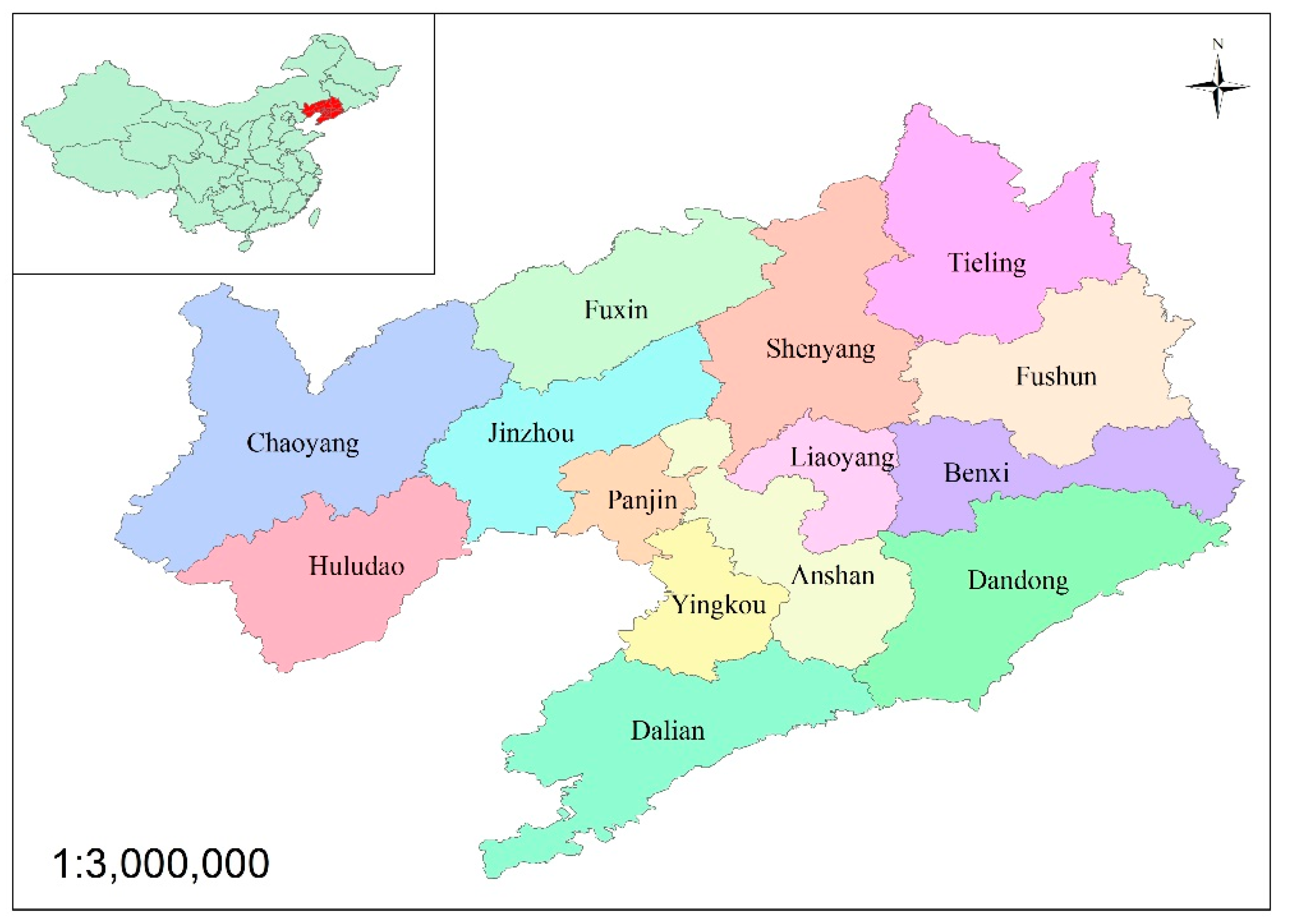
2.1. Overview of the Research Area
2.2. Methods
2.2.1. Regional Crop Production Water Footprint Model
2.2.2. Regional Crop Water Use Efficiency Model
2.3. Data
3. Results
3.1. Regional Crop Water Footprint Assessment
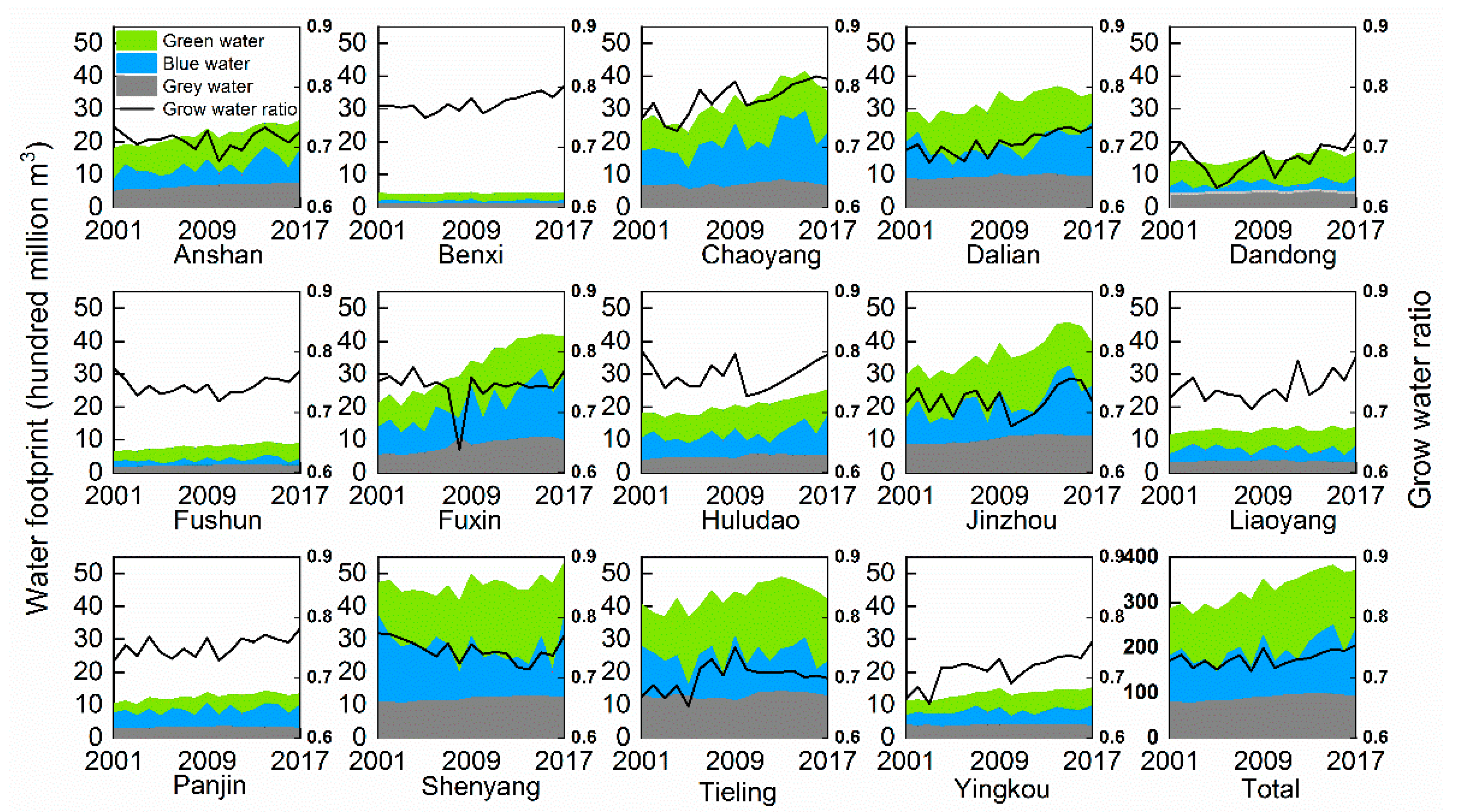
3.1.1. Characteristics of Regional Crop Water Footprint with Time
Changes of Regional Crop Growth Water Footprint
Changes of Regional Pollution Water Footprint
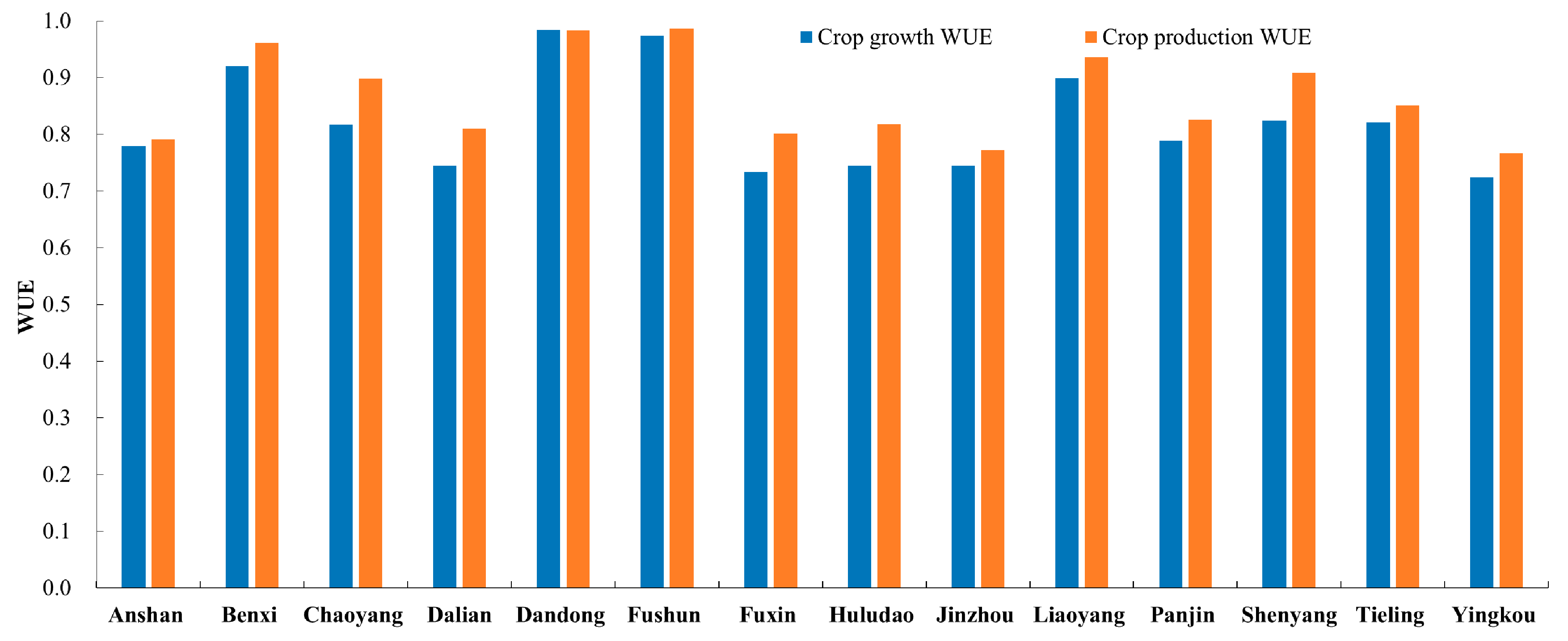
Changes of Regional Crop Production Water Footprint
3.1.2. Spatial Difference Analysis of Regional Crop Water Footprint
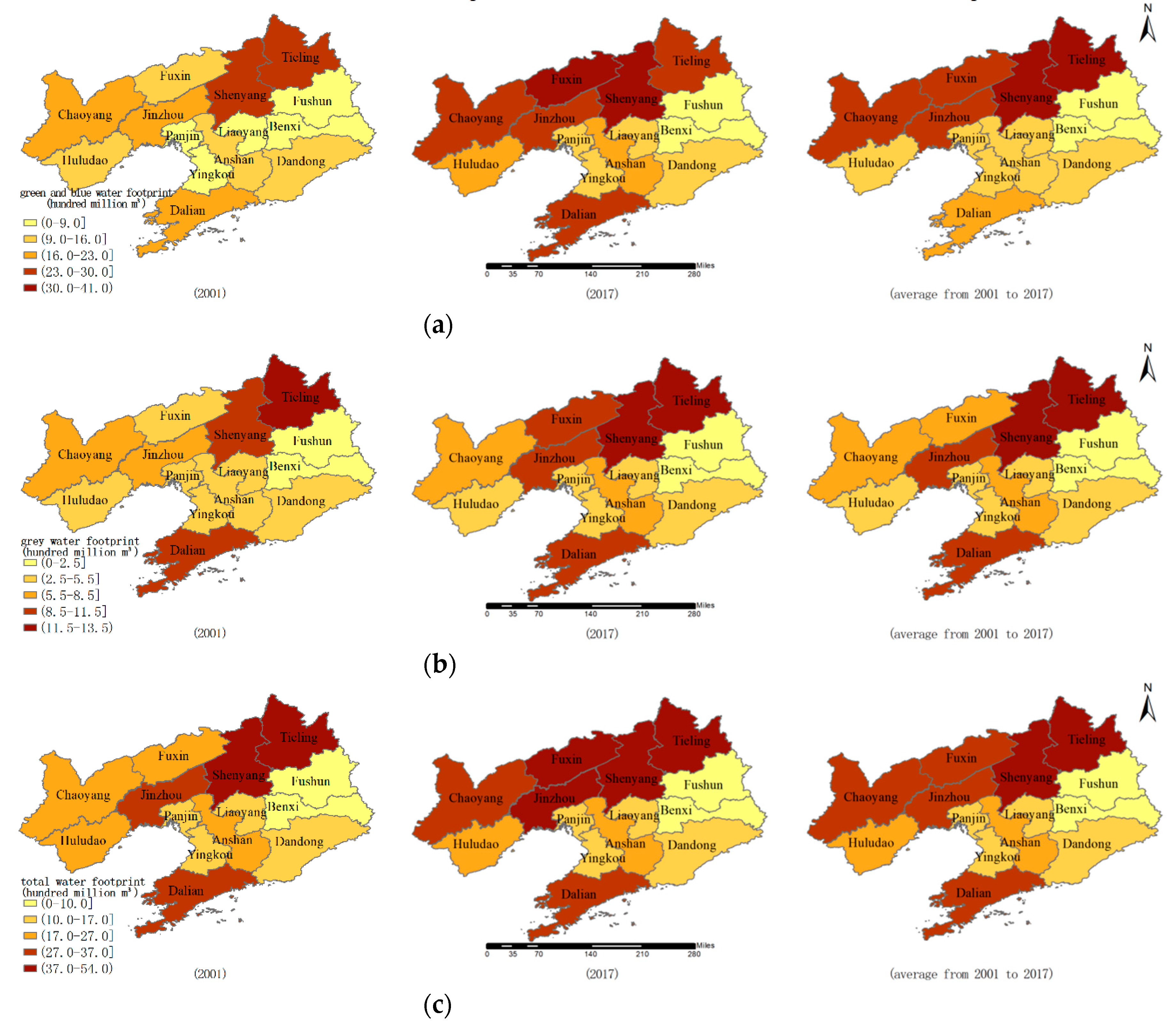
The Distribution of the Regional Crop Growth Water Footprint
The Distribution of Regional Pollution Water Footprint
The Distribution of Regional Production Water Footprint
3.2. Analysis of Crop Water Use Efficiency
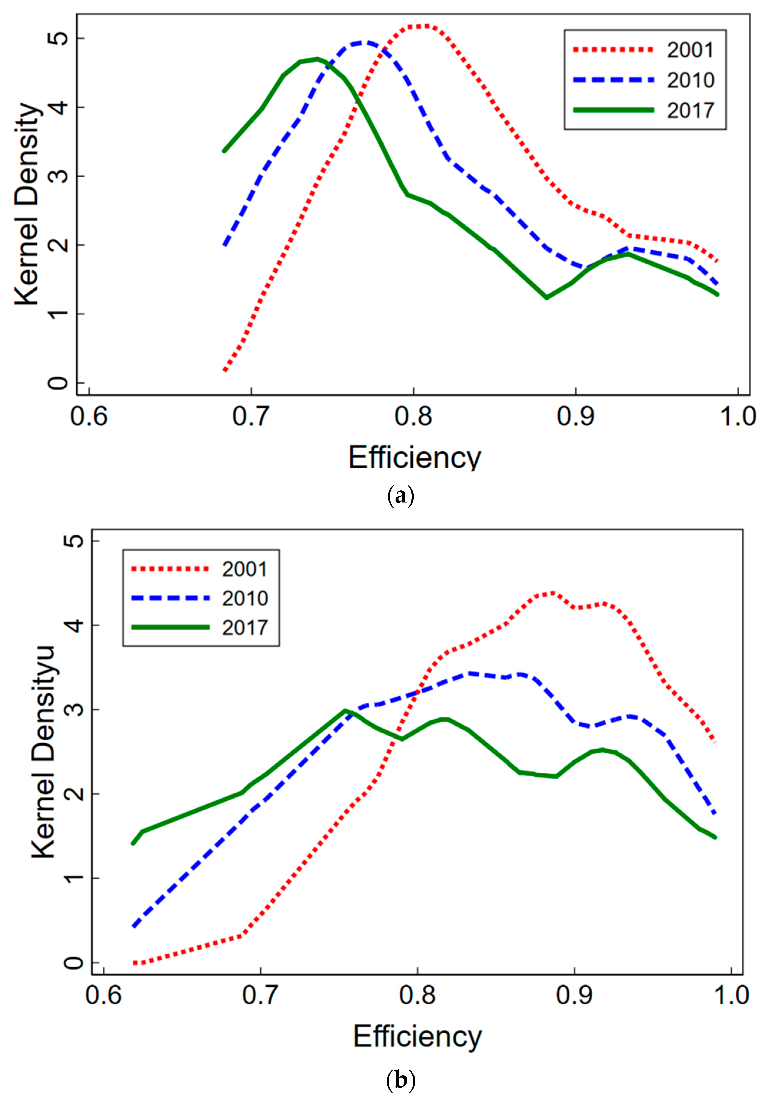
3.2.1. Dynamic Analysis of Crop Water Use Efficiency
Changes of Crop Growth Water Use Efficiency
Changes of the Crop Ecological Water Use Efficiency
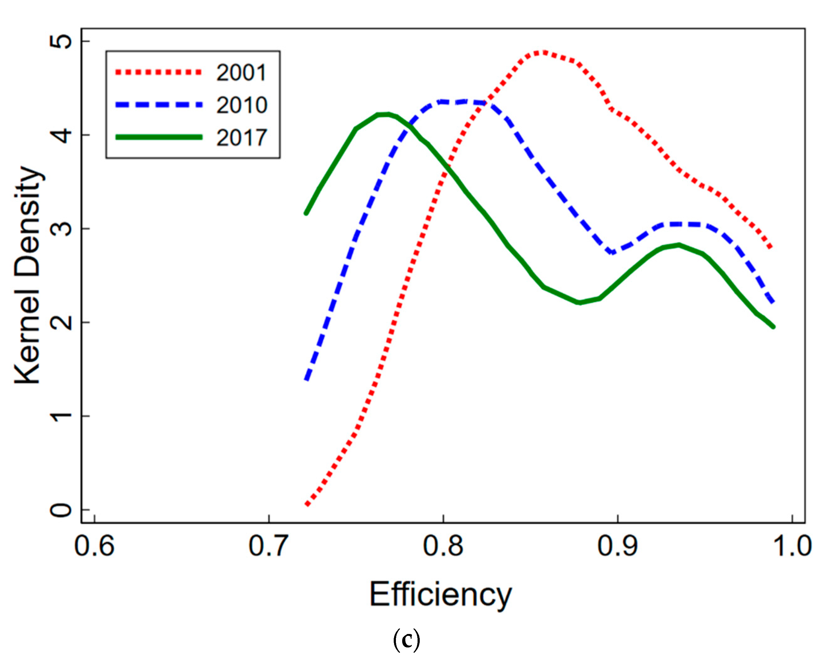
Changes of the Crop Production Water Use Efficiency
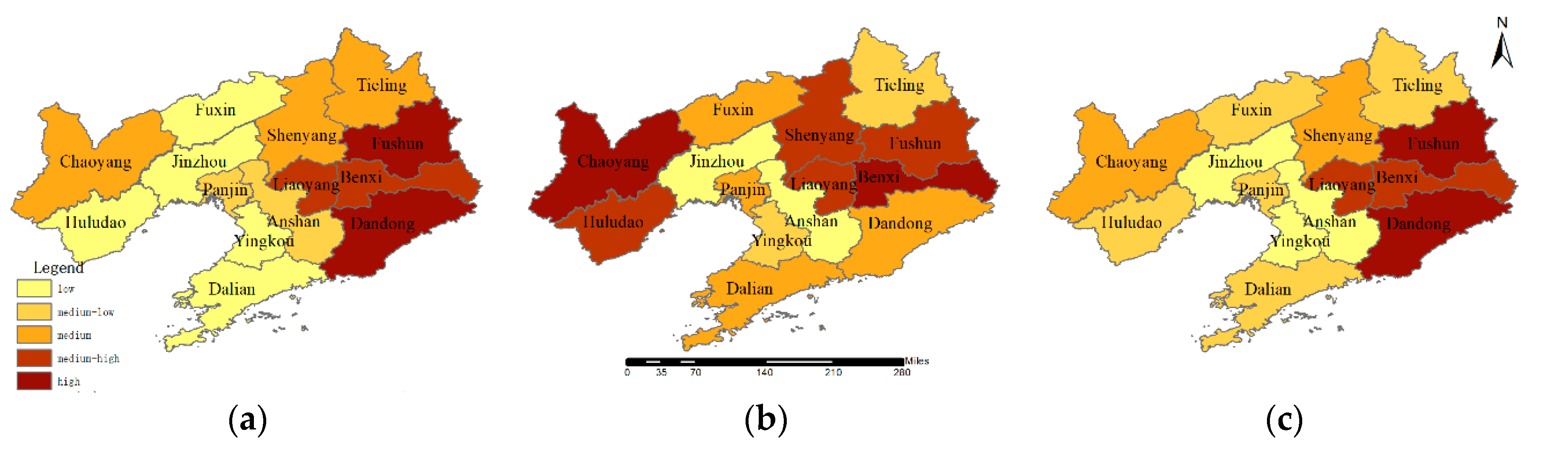
3.2.2. Spatial Analysis of Crop Water Use Efficiency
Distributions of Crop Growth Water Use Efficiency
Distributions of the Crop Ecological Water Use Efficiency
Changes of the Crop Production Water Use Efficiency
4. Discussion
5. Conclusions
Author Contributions
Funding
Data Availability Statement
Conflicts of Interest
References
- Niculita-Hirzel, H.; Goekce, S.; Jackson, C.E.; Suarez, G.; Amgwerd, L. Risk Exposure during Showering and Water-Saving Showers. Water 2021, 13, 2678. [Google Scholar] [CrossRef]
- Sieczka, A.; Bujakowski, F.; Falkowski, T.; Koda, E. Morphogenesis of a Floodplain as a Criterion for Assessing the Susceptibility to Water Pollution in an Agriculturally Rich Valley of a Lowland River. Water 2018, 10, 399. [Google Scholar] [CrossRef] [Green Version]
- Vaverka1, I.; Jakimiuk, A.; Trach, Y.; Koda, E.; Vaverková, M.D. Consumption and Savings of Drinking Water in Selected Objects. J. Ecol. Eng. 2021, 22, 13–25. [Google Scholar] [CrossRef]
- Sadr, S.K.; Memon, F.A.; Jain, A.; Gulati, S.; Duncan, A.P.; Hussein, W.; Savić, D.D.A.; Butler, D. An Analysis of Domestic Water Consumption in Jaipur, India. Br. J. Environ. Clim. Chang. 2016, 6, 97–115. [Google Scholar] [CrossRef] [Green Version]
- Feizizadeh, B.; Ronagh, Z.; Pourmoradian, S.; Hassan, A.G.; Lakes, T.; Thomas, B. An efficient GIS-based approach for sustainability assessment of urban drinking water consumption patterns: A study in Tabriz city, Iran. Sustain. Cities Soc. 2021, 64, 102584. [Google Scholar] [CrossRef]
- Hoekstra, A.Y.; Mekonnen, M.M. The water footprint of humanity. Proc. Natl. Acad. Sci. USA 2012, 109, 3232–3237. [Google Scholar] [CrossRef] [PubMed] [Green Version]
- Cao, X.; Zeng, W.; Wu, M.; Guo, X.; Wang, W. Hybrid analytical framework for regional agricultural water resource utilization and efficiency evaluation. Agric. Water Manag. 2020, 231, 106027. [Google Scholar] [CrossRef]
- Watto, M.A.; Mugera, A.W. Econometric estimation of groundwater irrigation efficiency of cotton cultivation farms in Pakistan. J. Hydrol. Reg. Stud. 2015, 4, 193–211. [Google Scholar] [CrossRef] [Green Version]
- Pereira, H.; Marques, R.C. An analytical review of irrigation efficiency measured using deterministic and stochastic models. Agric. Water Manag. 2017, 184, 28–35. [Google Scholar] [CrossRef]
- Grafton, R.Q.; Williams, J.; Perry, C.J.; Molle, F.; Ringler, C.; Steduto, P.; Udall, B.; Wheeler, S.A.; Wang, Y.; Garrick, D.; et al. The paradox of irrigation efficiency. Science 2018, 361, 748–750. [Google Scholar] [CrossRef] [Green Version]
- Han, S.; Hu, Q.; Yang, Y.; Yang, Y.; Zhou, X.; Li, H. Response of surface water quantity and quality to agricultural water use intensity in upstream Hutuo River Basin, China. Agric. Water Manag. 2019, 212, 378–387. [Google Scholar] [CrossRef]
- Duchemin, B.; Fieuzal, R.; Rivera, M.; Ezzahar, J.; Jarlan, L.; Rodriguez, J.; Hagolle, O.; Watts, C. Impact of Sowing Date on Yield and Water Use Efficiency of Wheat Analyzed through Spatial Modeling and FORMOSAT-2 Images. Remote Sens. 2015, 7, 5951–5979. [Google Scholar] [CrossRef] [Green Version]
- Lu, Y.; Zhang, X.; Chen, S.; Shao, L.; Sun, H. Changes in water use efficiency and water footprint in grain production over the past 35 years: A case study in the North China Plain. J. Clean. Prod. 2016, 116, 71–79. [Google Scholar] [CrossRef]
- Wang, Y.; Zhang, Y.; Zhou, S.; Wang, Z. Meta-analysis of no-tillage effect on wheat and maize water use efficiency in China. Sci. Total Environ. 2018, 635, 1372–1382. [Google Scholar] [CrossRef] [PubMed]
- Fishman, R.; Devineni, N.; Raman, S. Can improved agricultural water use efficiency save India’s groundwater? Environ. Res. Lett. 2015, 10, 084022. [Google Scholar] [CrossRef] [Green Version]
- Ren, C.; Guo, P.; Yang, G.; Li, R.; Liu, L. Spatial and Temporal Analyses of Water Resources Use Efficiency Based on Data Envelope Analysis and Malmquist Index: Case Study in Gansu Province, China. J. Water Resour. Plan. Manag. 2016, 142, 04016066. [Google Scholar] [CrossRef]
- Wang, W.; Yu, Z.; Zhang, W.; Shao, Q.; Zhang, Y.; Luo, Y.; Jiao, X.; Xu, J. Responses of rice yield, irrigation water requirement and water use efficiency to climate change in China: Historical simulation and future projections. Agric. Water Manag. 2014, 146, 249–261. [Google Scholar] [CrossRef]
- Marano, R.P.; Filippi, R.A. Water Footprint in paddy rice systems. Its determination in the provinces of Santa Fe and Entre Ríos, Argentina. Ecol. Indic. 2015, 56, 229–236. [Google Scholar] [CrossRef]
- Karandish, F.; Šimůnek, J. A comparison of the HYDRUS (2D/3D) and SALTMED models to investigate the influence of various water-saving irrigation strategies on the maize water footprint. Agric. Water Manag. 2019, 213, 809–820. [Google Scholar] [CrossRef] [Green Version]
- Xie, P.; Zhuo, L.; Yang, X.; Huang, H.; Wu, P. Spatial-temporal variations in blue and green water resources, water footprints and water scarcities in a large river basin: A case for the Yellow River Basin. J. Hydrol. 2020, 590, 125222. [Google Scholar] [CrossRef]
- Yonghu, F.; Liming, L.; Xiaoxing, Q.; Chengcheng, Y.; Shengjiao, L. Environmental effects evaluation for grain production based on grey water footprint in Dongting Lake area. Trans. Chin. Soc. Agric. Eng. 2015, 31, 152–160. [Google Scholar]
- Veettil, A.V.; Mishra, A.K. Water security assessment using blue and green water footprint concepts. J. Hydrol. 2016, 542, 589–602. [Google Scholar] [CrossRef]
- Chapagain, A.K.; Hoekstra, A.Y. The blue, green and grey water footprint of rice from production and consumption perspectives. Ecol. Econ. 2010, 70, 749–758. [Google Scholar] [CrossRef]
- Yoo, S.-H.; Choi, J.-Y.; Lee, S.-H.; Kim, T. Estimating water footprint of paddy rice in Korea. Paddy Water Environ. 2014, 12, 43–54. [Google Scholar] [CrossRef]
- Herath, I.; Green, S.; Singh, R.; Horne, D.; van der Zijpp, S.; Clothier, B. Water footprinting of agricultural products: A hydrological assessment for the water footprint of New Zealand’s wines. J. Clean. Prod. 2013, 41, 232–243. [Google Scholar] [CrossRef]
- Wang, X.; Yang, H.; Shi, M.; Zhou, D.; Zhang, Z. Managing stakeholders’ conflicts for water reallocation from agriculture to industry in the Heihe River Basin in Northwest China. Sci. Total Environ. 2015, 505, 823–832. [Google Scholar] [CrossRef] [PubMed]
- Novoa, V.; Ahumada-Rudolph, R.; Rojas, O.; Sáez, K.; Barrera, F.D.L.; Arumí, J.L. Understanding agricultural water footprint variability to improve water management in Chile. Sci. Total Environ. 2019, 670, 188–199. [Google Scholar] [CrossRef]
- Ababaei, B.; Etedali, H.R. Water footprint assessment of main cereals in Iran. Agric. Water Manag. 2017, 179, 401–411. [Google Scholar] [CrossRef]
- Wang, S.C.; Yeh, F.Y.; Eggert, R.G. Total-factor water efficiency of regions in China. Resour. Policy 2006, 31, 217–230. [Google Scholar] [CrossRef]
- Speelman, S.; D’Haese, M.; Buysse, J.; D’Haese, L. A measure for the efficiency of water use and its determinants, a case study of small-scale irrigation schemes in North-West Province, South Africa. Agric. Syst. 2008, 98, 31–39. [Google Scholar] [CrossRef]
- Scheierling, S.M.; Treguer, D.O.; Booker, J.F.; Elisabeth, D. How to Assess Agricultural Water Productivity? Looking for Water in the Agricultural Productivity and Efficiency Literature. In World Bank Policy Research Working Paper No. 6982; World Bank: Washington, DC, USA, 2014. [Google Scholar]
- Kaneko, S.; Tanaka, K.; Toyota, T.; Managi, S. Water efficiency of agricultural production in China: Regional comparison from 1999 to 2002. Int. J. Agric. Resour. Gov. Ecol. 2004, 3, 231–251. [Google Scholar] [CrossRef]
- Gadanakis, Y.; Bennett, R.; Park, J.; Areal, F.J. Improving productivity and water use efficiency: A case study of farms in England. Agric. Water Manag. 2015, 160, 22–32. [Google Scholar] [CrossRef] [Green Version]
- Zema, D.A.; Nicotra, A.; Mateos, L.; Zimbone, S.M. Improvement of the irrigation performance in Water Users Associations integrating data envelopment analysis and multi-regression models. Agric. Water Manag. 2018, 205, 38–49. [Google Scholar] [CrossRef]
- Njuki, E.; Bravo-Ureta, B.E. Irrigation water use and technical efficiencies: Accounting for technological and environmental heterogeneity in U.S. agriculture using random parameters. Water Resour. Econ. 2018, 24, 1–12. [Google Scholar] [CrossRef]
- Wang, F.; Yu, C.; Xiong, L.; Chang, Y. How can agricultural water use efficiency be promoted in China? A spatial-temporal analysis. Resour. Conserv. Recycl. 2019, 145, 411–418. [Google Scholar] [CrossRef]
- Geng, Q.; Ren, Q.; Nolan, R.H.; Wu, P.; Yu, Q. Assessing China’s agricultural water use efficiency in a green-blue water perspective: A study based on data envelopment analysis. Ecol. Indic. 2019, 96, 329–335. [Google Scholar] [CrossRef]
- Zhou, P.; Ang, B.W.; Zhou, D.Q. Measuring economy-wide energy efficiency performance: A parametric frontier approach. Appl. Energy 2012, 90, 196–200. [Google Scholar] [CrossRef]
- Siebert, S.; Döll, P. Quantifying blue and green virtual water contents in global crop production as well as potential production losses without irrigation. J. Hydrol. 2009, 384, 198–217. [Google Scholar] [CrossRef]
- Franke, N.; Hoekstra, A.Y.; Boyacioglu, H. Grey Water Footprint Accounting: Tier 1 Supporting Guidelines; Unesco-IHE: Delft, The Netherlands, 2017. [Google Scholar]
- Zeng, Z.; Liu, J.; Savenije, H.H.G. A simple approach to assess water scarcity integrating water quantity and quality. Ecol. Indic. 2013, 34, 441–449. [Google Scholar] [CrossRef]
- Battese, G.E.; Coelli, T.J. A Model for Technical Efficiency Effect in a Stochastic Frontier Production Functions for Panel Data. Empir. Econ. 1995, 20, 325–332. [Google Scholar] [CrossRef] [Green Version]
- Hipel, K.W.; McLeod, A. Time Series Modelling of Water Resources and Environmental Systems; Elsevier: Amsterdam, The Netherlands, 1994. [Google Scholar]


| Crop Growth Footprint | Crop Pollution Footprint | Crop Production Footprint | |||||||
|---|---|---|---|---|---|---|---|---|---|
| M-K Test | Long-Term Growth Rate (%) | Variation Coefficient (%) | M-K Test | Long-Term Growth Rate (%) | Variation coefficient (%) | M-K Test | Long-Term Growth Rate (%) | Variation Coefficient (%) | |
| Anshan | 4.08 ** | 2.34 | 12.95 | 5.31 ** | 2.63 | 11.94 | 4.49 ** | 2.42 | 12.27 |
| Benxi | 2.60 ** | 0.50 | 6.73 | −1.74 | −0.74 | 3.22 | 2.43 * | 0.23 | 5.16 |
| Chaoyang | 3.75 ** | 2.45 | 20.17 | 2.18 * | 0.02 | 11.01 | 3.83 ** | 1.92 | 17.54 |
| Dalian | 3.50 ** | 1.49 | 13.05 | 3.01 ** | 0.3 | 5.81 | 3.17 ** | 1.15 | 10.71 |
| Dandong | 2.92 ** | 1.67 | 12.43 | 3.05 ** | 0.54 | 6.80 | 3.01 ** | 1.34 | 9.76 |
| Fushun | 4.49 ** | 2.15 | 11.69 | 3.79 ** | 2.3 | 11.18 | 4.57 ** | 2.19 | 11.10 |
| Fuxin | 4.65 ** | 4.52 | 24.74 | 4.41 ** | 3.93 | 25.37 | 4.82 ** | 4.38 | 24.18 |
| Huludao | 3.83 ** | 2.12 | 13.66 | 3.01 ** | 2.35 | 12.51 | 4.49 ** | 2.17 | 12.22 |
| Jinzhou | 3.50 ** | 1.78 | 17.05 | 3.58 ** | 1.72 | 11.96 | 4.00 ** | 1.76 | 14.87 |
| Liaoyang | 2.18 * | 1.67 | 8.42 | −0.87 | −0.69 | 6.82 | 2.35 * | 1.10 | 5.80 |
| Panjin | 3.58 ** | 2.05 | 10.56 | 2.18 * | 0.22 | 6.56 | 3.58 ** | 1.60 | 9.00 |
| Shenyang | 1.28 | 2.54 | 8.82 | 4.16 ** | 0.84 | 6.45 | 2.18 * | 2.10 | 7.25 |
| Tieling | 2.68 ** | 0.49 | 10.92 | 1.44 | −0.37 | 7.08 | 2.68 ** | 0.22 | 8.74 |
| Yingkou | 4.08 ** | 2.84 | 13.01 | 0.99 | −0.09 | 4.96 | 4.08 ** | 2.00 | 10.01 |
| Prinvince | 4.24 ** | 2.13 | 12.40 | 4.00 ** | 0.97 | 8.30 | 4.49 ** | 1.82 | 11.07 |
| Variable | Growth WUE | Ecological WUE | Production WUE |
|---|---|---|---|
| value of agricultural production | 1.790 ** (−0.533) | 0.069 * (0.031) | 0.009 (0.032) |
| Agricultural practitioner | −0.021 (0.045) | 0.0190 (0.032) | −0.030 (0.036) |
| Crop sown Area | −0.047 (0.046) | −0.267 ** (0.062) | −0.484 ** (0.062) |
| Total power of crop machinery | −0.562 ** (0.094) | −0.026 (0.023) | 0.062 ** (0.025) |
| fertilizer useage | 0.103 ** (0.035) | −0.734 ** (0.044) | −0.481 ** (0.045) |
| Time | −0.373 ** (0.066) | 0.007 ** (0.002) | −0.004 (0.002) |
| Constant term | −0.007 * (0.003) | −1.158 ** (0.336) | 1.044 ** (0.372) |
| 0.078 ** (0.032) | 0.077 ** (0.032) | 0.048 * (0.021) | |
| γ | 0.922 ** (0.033) | 0.960 ** (0.017) | 0.931 ** (0.031) |
| −0.021 (0.013) | −0.036 ** (0.007) | −0.026 ** (0.011) | |
| Maximum likelihood value | 244.373 | 320.086 | 313.997 |
| LR | 130.369 | 297.070 | 177.901 |
Publisher’s Note: MDPI stays neutral with regard to jurisdictional claims in published maps and institutional affiliations. |
© 2022 by the authors. Licensee MDPI, Basel, Switzerland. This article is an open access article distributed under the terms and conditions of the Creative Commons Attribution (CC BY) license (https://creativecommons.org/licenses/by/4.0/).
Share and Cite
Piao, H.; Cheng, W.; Liu, H.; Lyu, J.; Zhang, X.; Sun, S. Crop Water-Saving Potential Based on the Stochastic Distance Function: The Case of Liaoning Province of China. Water 2022, 14, 432. https://doi.org/10.3390/w14030432
Piao H, Cheng W, Liu H, Lyu J, Zhang X, Sun S. Crop Water-Saving Potential Based on the Stochastic Distance Function: The Case of Liaoning Province of China. Water. 2022; 14(3):432. https://doi.org/10.3390/w14030432
Chicago/Turabian StylePiao, Huilan, Wanting Cheng, Haisheng Liu, Jie Lyu, Xudong Zhang, and Shijun Sun. 2022. "Crop Water-Saving Potential Based on the Stochastic Distance Function: The Case of Liaoning Province of China" Water 14, no. 3: 432. https://doi.org/10.3390/w14030432
APA StylePiao, H., Cheng, W., Liu, H., Lyu, J., Zhang, X., & Sun, S. (2022). Crop Water-Saving Potential Based on the Stochastic Distance Function: The Case of Liaoning Province of China. Water, 14(3), 432. https://doi.org/10.3390/w14030432