
Long-Term Series of Chlorophyll-a Concentration in Brazilian Semiarid Lakes from Modis Imagery


 ,
,  , and
, and
Abstract
1. Introduction
2. Materials and Methods
2.1. Study Sites
2.2. Field Data
2.3. MODIS Data
2.4. Modelling
2.5. Time Series
3. Results
3.1. Optical Properties
3.2. Modis Data Evaluation
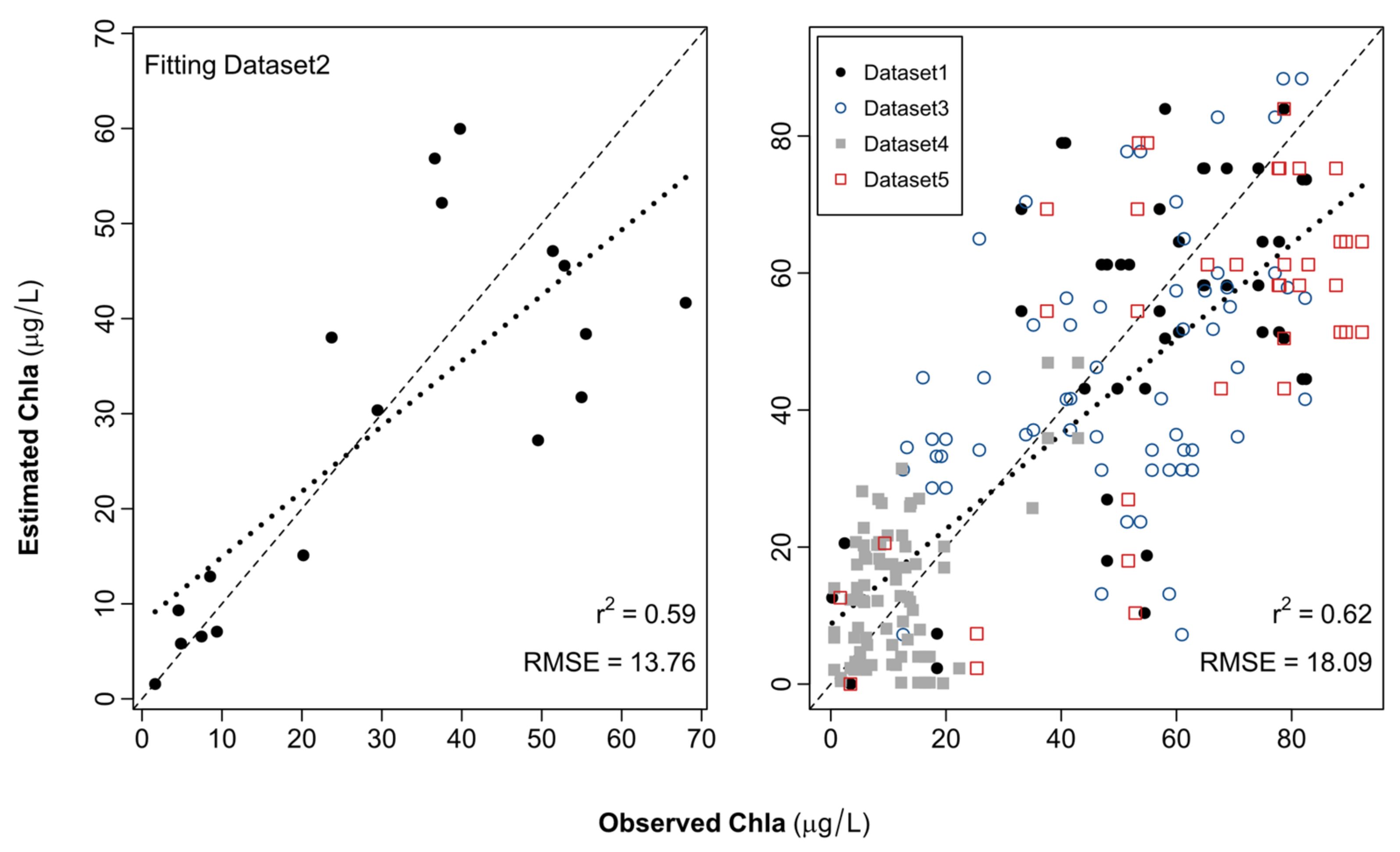
3.3. Modelling
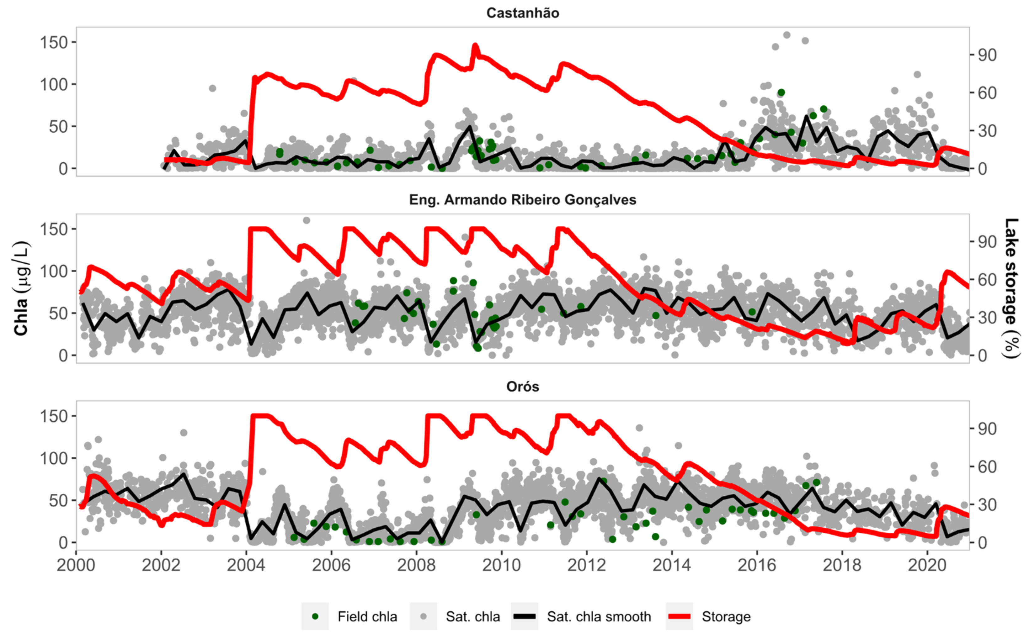
3.4. Time Series
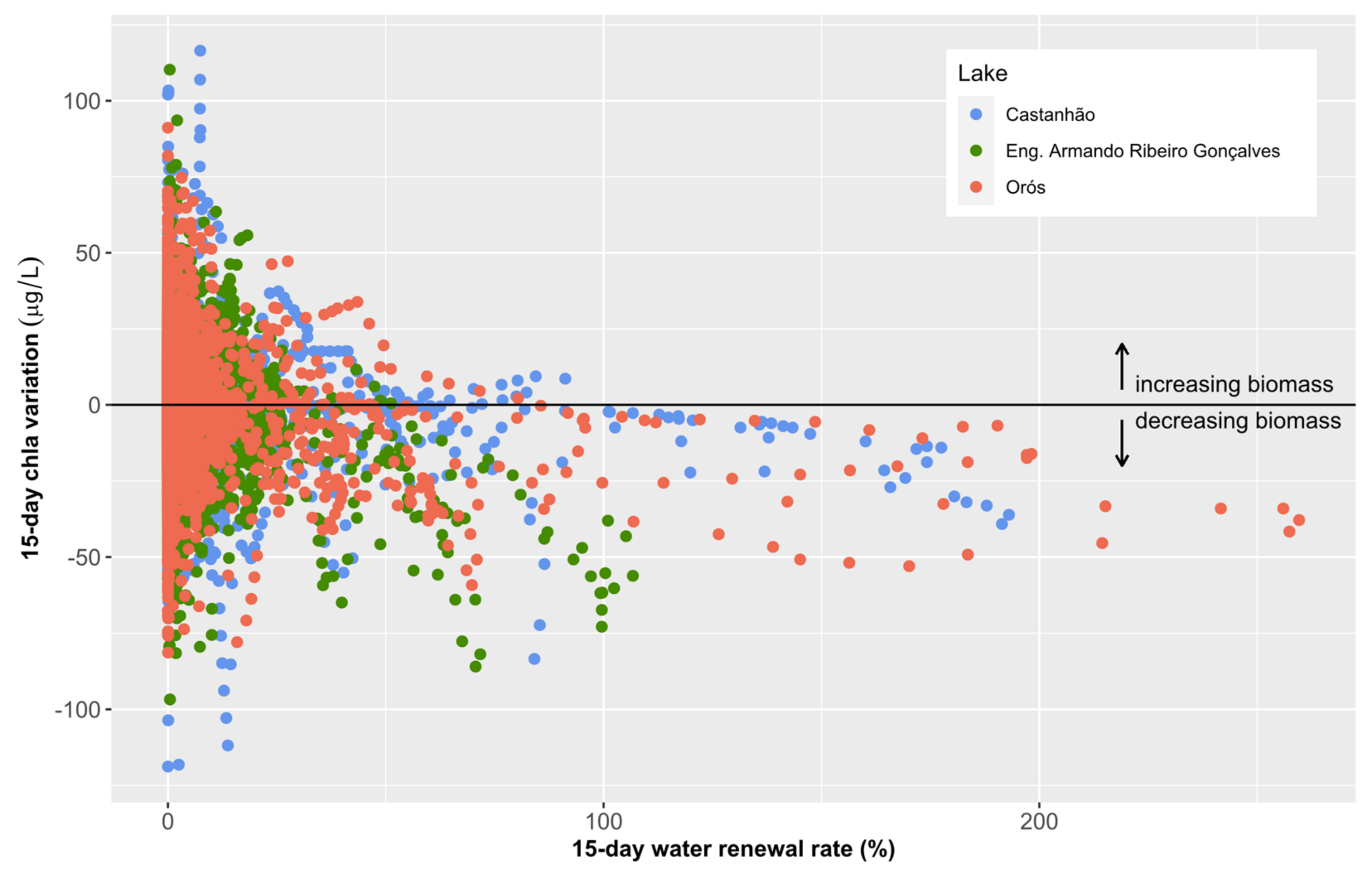
3.5. Hydraulic Effects
4. Discussion
Supplementary Materials
Author Contributions
Funding
Data Availability Statement
Acknowledgments
Conflicts of Interest
References
- Smith, V.H. Eutrophication of freshwater and coastal marine ecosystems: A global problem. Environ. Sci. Pollut. Res. Int. 2003, 10, 126–139. [Google Scholar] [CrossRef] [PubMed]
- Glibert, P.M. Eutrophication, harmful algae and biodiversity—Challenging paradigms in a world of complex nutrient changes. Mar. Pollut. Bull. 2017, 124, 591–606. [Google Scholar] [CrossRef]
- Carvalho, L.; Poikane, S.; Lyche Solheim, A.; Phillips, G.; Borics, G.; Catalan, J.; De Hoyos, C.; Drakare, S.; Dudley, B.J.; Järvinen, M.; et al. Strength and uncertainty of phytoplankton metrics for assessing eutrophication impacts in lakes. Hydrobiologia 2013, 704, 127–140. [Google Scholar] [CrossRef]
- Özkan, K.; Jeppesen, E.; Davidson, T.A.; Bjerring, R.; Johansson, L.S.; Søndergaard, M.; Lauridsen, T.L.; Svenning, J.C. Long-term trends and temporal synchrony in plankton richness, diversity and biomass driven by re-oligotrophication and climate across 17 Danish Lakes. Water 2016, 8, 427. [Google Scholar] [CrossRef]
- Thackeray, S.J.; Jones, I.D.; Maberly, S.C. Long-term change in the phenology of spring phytoplankton: Species-specific responses to nutrient enrichment and climatic change. J. Ecol. 2008, 96, 523–535. [Google Scholar] [CrossRef]
- Dubelaar, G.B.J.; Geerders, P.J.F.; Jonker, R.R. High frequency monitoring reveals phytoplankton dynamics. J. Environ. Monit. 2004, 6, 946–952. [Google Scholar] [CrossRef] [PubMed]
- Bowes, M.J.; Loewenthal, M.; Read, D.S.; Hutchins, M.G.; Prudhomme, C.; Armstrong, L.K.; Harman, S.A.; Wickham, H.D.; Gozzard, E.; Carvalho, L. Identifying multiple stressor controls on phytoplankton dynamics in the River Thames (UK) using high-frequency water quality data. Sci. Total Environ. 2016, 569–570, 1489–1499. [Google Scholar] [CrossRef]
- Strobl, R.O.; Robillard, P.D. Network design for water quality monitoring of surface freshwaters: A review. J. Environ. Manag. 2008, 87, 639–648. [Google Scholar] [CrossRef]
- Shutler, J.D.; Land, P.E.; Smyth, T.J.; Groom, S.B. Extending the MODIS 1-km ocean colour atmospheric correction to the MODIS 500-m bands and 500-m chlorophyll-a estimation towards coastal and estuarine monitoring. Remote Sens. Environ. 2007, 107, 521–532. [Google Scholar] [CrossRef]
- Shi, K.; Zhang, Y.; Zhu, G.; Liu, X.; Zhou, Y.; Xu, H.; Qin, B.; Liu, G.; Li, Y. Long-term remote monitoring of total suspended matter concentration in Lake Taihu using 250 m MODIS-Aqua data. Remote Sens. Environ. 2015, 164, 43–56. [Google Scholar] [CrossRef]
- Espinoza Villar, R.; Martinez, J.-M.; Guyot, J.-L.; Fraizy, P.; Armijos, E.; Crave, A.; Bazán, H.; Vauchel, P.; Lavado, W. The integration of field measurements and satellite observations to determine river solid loads in poorly monitored basins. J. Hydrol. 2012, 444–445, 221–228. [Google Scholar] [CrossRef]
- Wang, S.; Li, J.; Zhang, B.; Lee, Z.; Spyrakos, E.; Feng, L.; Liu, C.; Zhao, H.; Wu, Y.; Zhu, L.; et al. Changes of water clarity in large lakes and reservoirs across China observed from long-term MODIS. Remote Sens. Environ. 2020, 247, 111949. [Google Scholar] [CrossRef]
- Chakraborty, K.; Gupta, A.; Lotliker, A.A.; Tilstone, G. Evaluation of model simulated and MODIS-Aqua retrieved sea surface chlorophyll in the eastern Arabian Sea. Estuar. Coast. Shelf Sci. 2016, 181, 61–69. [Google Scholar] [CrossRef]
- Sarangi, R.K.; Devi, K.N. Space-based observation of chlorophyll, sea surface temperature, nitrate, and sea surface height anomaly over the Bay of Bengal and Arabian Sea. Adv. Sp. Res. 2017, 59, 33–44. [Google Scholar] [CrossRef]
- Modabberi, A.; Noori, R.; Madani, K.; Ehsani, A.H.; Danandeh Mehr, A.; Hooshyaripor, F.; Kløve, B. Caspian Sea is eutrophying: The alarming message of satellite data. Environ. Res. Lett. 2019, 15, 124047. [Google Scholar] [CrossRef]
- Hu, C.; Feng, L.; Lee, Z.; Davis, C.O.; Mannino, A.; McClain, C.R.; Franz, B.A. Dynamic range and sensitivity requirements of satellite ocean color sensors: Learning from the past. Appl. Opt. 2012, 51, 6045. [Google Scholar] [CrossRef]
- Tarrant, P.E.; Amacher, J.A.; Neuer, S. Assessing the potential of Medium-Resolution Imaging Spectrometer (MERIS) and Moderate-Resolution Imaging Spectroradiometer (MODIS) data for monitoring total suspended matter in small and intermediate sized lakes and reservoirs. Water Resour. Res. 2010, 46, 1–7. [Google Scholar] [CrossRef]
- De Moraes Novo, E.M.L.; de Farias Barbosa, C.C.; Freitas, R.M.; Shimabukuro, Y.E.; Melack, J.M.; Pereira-Filho, W. Seasonal changes in chlorophyll distributions in Amazon floodplain lakes derived from MODIS images. Limnology 2006, 7, 153–161. [Google Scholar] [CrossRef]
- Zhang, Y.; Lin, S.; Qian, X.; Wang, Q.; Qian, Y.; Liu, J.; Ge, Y. Temporal and spatial variability of chlorophyll a concentration in Lake Taihu using MODIS time-series data. Hydrobiologia 2011, 661, 235–250. [Google Scholar] [CrossRef]
- Ogashawara, I.; Alcântara, E.H.; Curtarelli, M.P.; Adami, M.; Nascimento, R.F.F.; Souza, A.F.; Stech, J.L.; Kampel, M. Performance analysis of MODIS 500-m spatial resolution products for estimating chlorophyll-a concentrations in oligo- to meso-trophic waters case study: Itumbiara reservoir, Brazil. Remote Sens. 2014, 6, 1634–1653. [Google Scholar] [CrossRef]
- Lins, R.; Martinez, J.-M.; Motta Marques, D.; Cirilo, J.; Medeiros, P.; Fragoso Júnior, C. A Multivariate Analysis Framework to Detect Key Environmental Factors Affecting Spatiotemporal Variability of Chlorophyll-a in a Tropical Productive Estuarine-Lagoon System. Remote Sens. 2018, 10, 853. [Google Scholar] [CrossRef]
- Zhang, Y.; Ma, R.; Duan, H.; Loiselle, S.; Zhang, M.; Xu, J. A novel MODIS algorithm to estimate chlorophyll a concentration in eutrophic turbid lakes. Ecol. Indic. 2016, 69, 138–151. [Google Scholar] [CrossRef]
- Bouvy, M.; Falcão, D.; Marinho, M.; Pagano, M.; Moura, A. Occurrence of Cylindrospermopsis (Cyanobacteria) in 39 Brazilian tropical reservoirs during the 1998 drought. Aquat. Microb. Ecol. 2000, 23, 13–27. [Google Scholar] [CrossRef]
- Costa, I.A.S.; Cunha, S.R.D.S.; Panosso, R.; Araújo, M.F.F.; Melo, J.L.d.S.; Eskinazi-Sant’Anna, E.M. Dinâmica de Cianobactérias em reservatórios eutróficos do semi-árido do Rio Grande do Norte. Oecologia Aust. 2009, 13, 382–401. [Google Scholar] [CrossRef]
- Huszar, V.; Silva, L.; Marinho, M.; Domingos, P.; Sant’Anna, C. Cyanoprokaryote assemblages in eight productive tropical Brazilian waters. Hydrobiologia 2000, 424, 67–77. [Google Scholar] [CrossRef]
- Brasil, J.; Attayde, J.L.; Vasconcelos, F.R.; Dantas, D.D.F.; Huszar, V.L.M. Drought-induced water-level reduction favors cyanobacteria blooms in tropical shallow lakes. Hydrobiologia 2016, 770, 145–164. [Google Scholar] [CrossRef]
- Krol, M.S.; Bronstert, A. Regional integrated modelling of climate change impacts on natural resources and resource usage in semi-arid Northeast Brazil. Environ. Model. Softw. 2007, 22, 259–268. [Google Scholar] [CrossRef]
- Uvo, C.B.; Repelli, C.A.; Zebiak, S.E.; Kushnir, Y. The relationships between tropical Pacific and Atlantic SST and northeast Brazil monthly precipitation. J. Clim. 1998, 11, 551–562. [Google Scholar] [CrossRef]
- Medeiros, P.H.A.; Araújo, J.C. de Temporal variability of rainfall in a semiarid environment in Brazil and its effect on sediment transport processes. J. Soils Sediments 2014, 14, 1216–1223. [Google Scholar] [CrossRef]
- Barbosa, J.E.d.L.; Medeiros, E.S.F.; Brasil, J.; Cordeiro, R.d.S.; Crispim, M.C.B.; da Silva, G.H.G. Aquatic systems in semi-arid Brazil: Limnology and management. Acta Limnol. Bras. 2012, 24, 103–118. [Google Scholar] [CrossRef]
- COGERH. Anuário do Monitoramento Quantitativo dos Principais Açudes do Estado do Ceará: 2017; COGERH: Fortaleza, Brazil, 2018. [Google Scholar]
- Stich, H.B.; Brinker, A. Less is better: Uncorrected versus pheopigment-corrected photometric chlorophyll-a estimation. Arch. Hydrobiol. 2005, 162, 111–120. [Google Scholar] [CrossRef]
- Jespersen, A.M.; Christoffersen, K. Measurements of chlorophyll-a from phytoplankton using ethanol as extraction solvent. Arch. Hydrobiol. 1987, 109, 445–454. [Google Scholar]
- Jeffrey, S.W.; Humphrey, G.F. New spectrophotometric equations for determining chlorophylls a, b, c1 and c2 in higher plants, algae and natural phytoplankton. Biochem. Physiol. Pflanz. 1975, 167, 191–194. [Google Scholar] [CrossRef]
- APHA; AWWA; WEF. Standard Methods for the Examination of Water and Wastewater, 21st ed.; American Public Health Association: Washington, DC, USA, 2005. [Google Scholar]
- Mobley, C.D. Estimation of the remote-sensing reflectance from above-surface measurements. Appl. Opt. 1999, 38, 7442–7455. [Google Scholar] [CrossRef]
- Vermote, E. MOD09A1 MODIS/Terra Surface Reflectance 8-Day L3 Global 500 m SIN Grid V006. Available online: http://doi.org/10.5067/MODIS/MOD09A1.006 (accessed on 20 December 2021).
- Gorelick, N.; Hancher, M.; Dixon, M.; Ilyushchenko, S.; Thau, D.; Moore, R. Google Earth Engine: Planetary-scale geospatial analysis for everyone. Remote Sens. Environ. 2017, 202, 18–27. [Google Scholar] [CrossRef]
- Wang, S.; Li, J.; Zhang, B.; Shen, Q.; Zhang, F.; Lu, Z. A simple correction method for the MODIS surface reflectance product over typical inland waters in China. Int. J. Remote Sens. 2016, 37, 6076–6096. [Google Scholar] [CrossRef]
- Allan, M.G.; Hamilton, D.P.; Hicks, B.J.; Brabyn, L. Landsat remote sensing of chlorophyll a concentrations in central North Island lakes of New Zealand. Int. J. Remote Sens. 2011, 32, 2037–2055. [Google Scholar] [CrossRef]
- Brezonik, P.; Menken, K.D.; Bauer, M. Landsat-based remote sensing of lake water quality characteristics, including chlorophyll and colored dissolved organic matter (CDOM). Lake Reserv. Manag. 2005, 21, 373–382. [Google Scholar] [CrossRef]
- Lim, J.; Choi, M. Assessment of water quality based on Landsat 8 operational land imager associated with human activities in Korea. Environ. Monit. Assess. 2015, 187, 1–17. [Google Scholar] [CrossRef] [PubMed]
- Nazeer, M.; Nichol, J.E. Development and application of a remote sensing-based Chlorophyll-a concentration prediction model for complex coastal waters of Hong Kong. J. Hydrol. 2016, 532, 80–89. [Google Scholar] [CrossRef]
- Gitelson, A.A.; Schalles, J.F.; Hladik, C.M. Remote chlorophyll-a retrieval in turbid, productive estuaries: Chesapeake Bay case study. Remote Sens. Environ. 2007, 109, 464–472. [Google Scholar] [CrossRef]
- Le, C.; Li, Y.; Zha, Y.; Sun, D.; Huang, C.; Lu, H. A four-band semi-analytical model for estimating chlorophyll a in highly turbid lakes: The case of Taihu Lake, China. Remote Sens. Environ. 2009, 113, 1175–1182. [Google Scholar] [CrossRef]
- Thornton, J.; Rast, W. A test of hypotheses relating to the comparative limnology and assessment of eutrophication in semi-arid man-made lakes. In Comparative Reservoir Limnology and Water Quality Management; Straskraba, M., Tundisi, J., Duncan, A., Eds.; Springer: Dordrecht, The Netherlands, 1993; pp. 1–24. [Google Scholar]
- Cunha, D.G.F.; do Carmo Calijuri, M.; Lamparelli, M.C. A trophic state index for tropical/subtropical reservoirs (TSItsr). Ecol. Eng. 2013, 60, 126–134. [Google Scholar] [CrossRef]
- Ma, B.; Wu, L.; Zhang, X.; Li, X.; Liu, Y.; Wang, S. Locally adaptive unmixing method for lake-water area extraction based on MODIS 250 m bands. Int. J. Appl. Earth Obs. Geoinf. 2014, 33, 109–118. [Google Scholar] [CrossRef]
- Gebru, H.G.; Melesse, A.M.; Gebremariam, A.G. Double-stage linear spectral unmixing analysis for improving accuracy of sediment concentration estimation from MODIS data: The case of Tekeze River, Ethiopia. Model. Earth Syst. Environ. 2020, 6, 407–416. [Google Scholar] [CrossRef]
- Le, C.; Hu, C.; English, D.; Cannizzaro, J.; Chen, Z.; Feng, L.; Boler, R.; Kovach, C. Towards a long-term chlorophyll-a data record in a turbid estuary using MODIS observations. Prog. Oceanogr. 2013, 109, 90–103. [Google Scholar] [CrossRef]
- Zhang, M.; Ma, R.; Li, J.; Zhang, B.; Duan, H. A validation study of an improved SWIR iterative atmospheric correction algorithm for MODIS-aqua measurements in lake Taihu, China. IEEE Trans. Geosci. Remote Sens. 2014, 52, 4686–4695. [Google Scholar] [CrossRef]
- Gitelson, A.A.; Dall’Olmo, G.; Moses, W.J.; Rundquist, D.C.; Barrow, T.; Fisher, T.R.; Gurlin, D.; Holz, J. A simple semi-analytical model for remote estimation of chlorophyll-a in turbid waters: Validation. Remote Sens. Environ. 2008, 112, 3582–3593. [Google Scholar] [CrossRef]
- Dörnhöfer, K.; Oppelt, N. Remote sensing for lake research and monitoring—Recent advances. Ecol. Indic. 2016, 64, 105–122. [Google Scholar] [CrossRef]
- Ligi, M.; Kutser, T.; Kallio, K.; Attila, J.; Koponen, S.; Paavel, B.; Soomets, T.; Reinart, A. Testing the performance of empirical remote sensing algorithms in the Baltic Sea waters with modelled and in situ reflectance data. Oceanologia 2017, 59, 57–68. [Google Scholar] [CrossRef]
- Angelini, R.; Bini, L.M.; Starling, F.L.R.M. Efeitos de diferentes intervenções no processo de eutrofização do lago Paranoá (Brasília-DF). Oecologia Aust. 2008, 12, 564–571. [Google Scholar] [CrossRef][Green Version]
- Vanni, M.J.; Andrews, J.S.; Renwick, W.H.; Gonzalez, M.J.; Noble, S.J. Nutrient and light limitation of reservoir phytoplankton in relation to storm-mediated pulses in stream discharge. Arch. Hydrobiol. 2006, 167, 421–445. [Google Scholar] [CrossRef]
- Naselli-Flores, L. Man-made lakes in Mediterranean semi-arid climate: The strange case of Dr Deep Lake and Mr Shallow Lake. Hydrobiologia 2003, 506–509, 13–21. [Google Scholar] [CrossRef]
- Rangel, L.M.; Silva, L.H.S.; Rosa, P.; Roland, F.; Huszar, V.L.M. Phytoplankton biomass is mainly controlled by hydrology and phosphorus concentrations in tropical hydroelectric reservoirs. Hydrobiologia 2012, 693, 13–28. [Google Scholar] [CrossRef]
- Harris, G.P.; Baxter, G. Interannual variability in phytoplankton biomass and species composition in a subtropical reservoir. Freshw. Biol. 1996, 35, 545–560. [Google Scholar] [CrossRef]
- De Castro Medeiros, L.; Mattos, A.; Lürling, M.; Becker, V. Is the future blue-green or brown? The effects of extreme events on phytoplankton dynamics in a semi-arid man-made lake. Aquat. Ecol. 2015, 49, 293–307. [Google Scholar] [CrossRef]
- Bouvy, M.; Nascimento, S.M.; Molica, R.J.R.; Ferreira, A.; Huszar, V.; Azevedo, S.M.F.O. Limnological features in Tapacurá reservoir (northeast Brazil) during a severe drought. Hydrobiologia 2003, 493, 115–130. [Google Scholar] [CrossRef]
- Gomes, L.C.; Miranda, L.E. Hydrologic and climatic regimes limit phytoplankton biomass in reservoirs of the Upper Paraná River Basin, Brazil. Hydrobiologia 2001, 457, 205–214. [Google Scholar] [CrossRef]
- Lins, R.P.M.; de Ceballos, B.S.O.; Lopez, L.C.S.; Barbosa, L.G. Phytoplankton functional groups in a tropical reservoir in the Brazilian semiarid region. Int. J. Trop. Biol. 2017, 65, 1129–1141. [Google Scholar] [CrossRef]
- Soares, M.C.S.; Marinho, M.M.; Huszar, V.L.M.; Branco, C.W.C.; Azevedo, S.M.F.O. The effects of water retention time and watershed features on the limnology of two tropical reservoirs in Brazil. Lakes Reserv. Res. Manag. 2008, 13, 257–269. [Google Scholar] [CrossRef]
- Abell, J.M.; Hamilton, D.P. Biogeochemical processes and phytoplankton nutrient limitation in the inflow transition zone of a large eutrophic lake during a summer rain event. Ecohydrology 2015, 8, 243–262. [Google Scholar] [CrossRef]
- Calijuri, M.; Dos Santos, A. Temporal variations in phytoplankton primary production in a tropical reservoir (Barra Bonita, SP—Brazil). Hydrobiologia 2001, 445, 11–26. [Google Scholar] [CrossRef]
- Costa, M.R.A.; Attayde, J.L.; Becker, V. Effects of water level reduction on the dynamics of phytoplankton functional groups in tropical semi-arid shallow lakes. Hydrobiologia 2016, 778, 75–89. [Google Scholar] [CrossRef]
- Rocha-Jr, C.A.N.; Costa, M.R.A.; Menezes, R.F.; Attayde, J.L.; Becker, V. Water volume reduction increases eutrophication risk in tropical semi-arid reservoirs. Acta Limnol. Bras. 2018, 30. [Google Scholar] [CrossRef]
- Noori, R.; Ansari, E.; Bhattarai, R.; Tang, Q.; Aradpour, S.; Maghrebi, M.; Torabi Haghighi, A.; Bengtsson, L.; Kløve, B. Complex dynamics of water quality mixing in a warm mono-mictic reservoir. Sci. Total Environ. 2021, 777, 146097. [Google Scholar] [CrossRef] [PubMed]
- Noori, R.; Ansari, E.; Jeong, Y.W.; Aradpour, S.; Maghrebi, M.; Hosseinzadeh, M.; Bateni, S.M. Hyper-nutrient enrichment status in the sabalan lake, iran. Water 2021, 13, 2874. [Google Scholar] [CrossRef]
- Naselli-Flores, L.; Barone, R. Water-level fluctuations in Mediterranean reservoirs: Setting a dewatering threshold as a management tool to improve water quality. Hydrobiologia 2005, 548, 85–99. [Google Scholar] [CrossRef]
- Marengo, J.A.; Jones, R.; Alves, L.M.; Valverde, M.C. Future change of temperature and precipitation extremes in South America as derived from the PRECIS regional climate modeling system. Int. J. Climatol. 2009, 29, 2241–2255. [Google Scholar] [CrossRef]
- Costa, M.R.A.; Menezes, R.F.; Sarmento, H.; Attayde, J.L.; Sternberg, L.d.S.L.; Becker, V. Extreme drought favors potential mixotrophic organisms in tropical semi-arid reservoirs. Hydrobiologia 2019, 831, 43–54. [Google Scholar] [CrossRef]


| Lake | ID | Surface Area (km2) | Storage Capacity (hm3) | Mean Depth (m) | Location (Coordinates) |
|---|---|---|---|---|---|
| Castanhão | CAST | 441.00 | 6700 | 15 | 5.500° S, 38.470° W |
| Orós | OROS | 350.00 | 1940 | 6 | 6.250° S, 38.940° W |
| Eng. Armando Ribeiro Gonçalves | EARG | 195.00 | 2400 | 12 | 5.690° S, 36.880° W |
| Banabuiu | BANB | 102.00 | 1700 | 17 | 5.360° S, 38.950° W |
| Pedras Brancas | PEDB | 72.88 | 434 | 6 | 5.130° S, 38.880° W |
| Pacoti | PACT | 37.00 | 370 | 10 | 4.040° S, 38.540° W |
| Pacajus | PACJ | 35.56 | 240 | 7 | 4.220° S, 38.400° W |
| Santa Cruz do Apodi | SCAP | 34.13 | 600 | 18 | 5.770° S, 37.810° W |
| Umari | UMAR | 29.23 | 293 | 10 | 5.700° S, 37.240° W |
| Piató Lake | PIAT | 15.53 | 96 | 6 | 5.520° S, 36.940° W |
| Aracoiaba | ARAC | 15.06 | 171 | 11 | 4.400° S, 38.710° W |
| Mendobim | MEND | 9.70 | 76 | 8 | 5.650° S, 36.932° W |
| Malcozinhado | MALC | 1.85 | 38 | 21 | 4.108° S, 38.295° W |
| Statistics | Dataset 1 | Dataset 2 | Dataset 3 | Dataset 4 | Dataset 5 | ||
|---|---|---|---|---|---|---|---|
| Chla | SSS | ISS | Chla | Chla | Chla | Chla | |
| n | 73 | 48 | 37 | 18 | 72 | 47 | 219 |
| min | 0.2 | 0.5 | 0.0 | 1.6 | 0.0 | 7.2 | 0.0 |
| median | 38.4 | 8.2 | 0.5 | 33.0 | 51.5 | 51.4 | 10.4 |
| mean | 37.4 | 10.3 | 2.6 | 30.9 | 51.1 | 48.3 | 18.1 |
| max | 101.0 | 39.0 | 18.7 | 68.0 | 229.9 | 82.3 | 251.6 |
| std. dev. | 25.8 | 8.1 | 5.2 | 21.5 | 41.6 | 21.2 | 27.7 |
| # | Tested Model | n | r2 | RMSE | Ref. |
|---|---|---|---|---|---|
| 1 | 9.17 − 44 × IR + 9800 × IR2 | 145 | 0.907 | 7.48 | [19] |
| 2 | 10 × (IR/R)1.8416 | 26 | 0.83 | 15.24 | [21] |
| 3 | 104,401.57 × R1.9742 | 16 | 0.954 | - | [40] |
| 4 | 6.71 + 0.0537 × B − 1.559 × B/R | 15 | 0.88 | - | [41] |
| 5 | 21.79 − 0.1675 × B − 3.855 × B/G | 15 | 0.86 | - | [41] |
| 6 | 63.434 + 153.778 × B − 803.31 × G + 239.639 × R | 44 | 0.71 | - | [42] |
| 7 | 49.057 + 63.832 × B − 236.05 × G − 110.046 × IR | 44 | 0.73 | - | [42] |
| 8 | 49.428 − 183.033 × G − 103.798 × IR | 44 | 0.73 | - | [42] |
| 9 | 51.922 − 366.287 × G + 184.622 × R − 116.926 × IR | 44 | 0.74 | - | [42] |
| 10 | 54.658 + 520.451 × B − 1221.89 × G + 611.115 × R − 198.199 × IR | 44 | 0.77 | 6.32 | [42] |
| 11 | 1.31 + 0.64 × (G/B2) | 85 | 0.84 | 1.78 | [43] |
| 12 | 6.6 + 79.05 × BNDBI + 562.4 × BNDBI2 + 71.86 × BNDBI3 + 982.3 × BNDBI4 | 114 | 0.925 | 1.82 | [22] |
| # | Chla Predictive Model | Fitting | Validation | |||
|---|---|---|---|---|---|---|
| n | r2 | n | r2 | RMSE | ||
| 1 | 1624 × exp(−0.005497 × R − 993.9 × G−1) | 18 | 0.59 | 86 | 0.62 | 18.1 |
| 2 | 118 − 115.3 × R/G − 4084 × R−1 | 18 | 0.50 | 86 | 0.60 | 20.7 |
| 3 | 88.87 − 0.1015 × R2/G − 14,170 × G−1 | 18 | 0.65 | 86 | 0.58 | 19.8 |
| 4 | 108.8 − 0.1045 × R − 17,160 × 1/G | 18 | 0.66 | 86 | 0.55 | 20.1 |
| 5 | 171.4 × exp(−0.004107 × R2/G − 222.7 × R−1) | 18 | 0.70 | 86 | 0.53 | 22.5 |
| 6 | 108.1 − 0.1958 × Rh − 17,390 × G−1 | 18 | 0.66 | 86 | 0.46 | 21.3 |
| 7 | 66.19 − 0.07716 × R2/G − 3507 × R−1 | 18 | 0.52 | 86 | 0.41 | 23.4 |
| Lake | Records | Freq. (%) | Records/Month |
|---|---|---|---|
| Eng. Armando Ribeiro Gonçalves (EARG) | 1620 | 63 | 19.3 |
| Orós (OROS) | 1463 | 57 | 17.4 |
| Castanhão (CAST) | 929 | 36 | 11.1 |
| Pacajus (PACJ) | 588 | 23 | 7.0 |
| Piató (PIAT) | 532 | 21 | 6.3 |
| Santa Cruz do Apodi (SCAP) | 503 | 20 | 6.0 |
| Pacoti (PACT) | 394 | 15 | 4.7 |
| Boqueirão de Pedras Brancas (PEDB) | 357 | 14 | 4.3 |
| Mendobim (MEND) | 273 | 11 | 3.3 |
| Umari (UMAR) | 143 | 6 | 1.7 |
| Banabuiú (BANB) | 138 | 5 | 1.6 |
| Aracoiaba (ARAC) | 98 | 4 | 1.2 |
| Malcozinhado (MALC) | 64 | 3 | 0.8 |
Publisher’s Note: MDPI stays neutral with regard to jurisdictional claims in published maps and institutional affiliations. |
© 2022 by the authors. Licensee MDPI, Basel, Switzerland. This article is an open access article distributed under the terms and conditions of the Creative Commons Attribution (CC BY) license (https://creativecommons.org/licenses/by/4.0/).
Share and Cite
Ventura, D.L.T.; Martinez, J.-M.; de Attayde, J.L.; Martins, E.S.P.R.; Brandini, N.; Moreira, L.S. Long-Term Series of Chlorophyll-a Concentration in Brazilian Semiarid Lakes from Modis Imagery. Water 2022, 14, 400. https://doi.org/10.3390/w14030400
Ventura DLT, Martinez J-M, de Attayde JL, Martins ESPR, Brandini N, Moreira LS. Long-Term Series of Chlorophyll-a Concentration in Brazilian Semiarid Lakes from Modis Imagery. Water. 2022; 14(3):400. https://doi.org/10.3390/w14030400
Chicago/Turabian StyleVentura, Dhalton Luiz Tosetto, Jean-Michel Martinez, José Luiz de Attayde, Eduardo Sávio Passos Rodrigues Martins, Nilva Brandini, and Luciane Silva Moreira. 2022. "Long-Term Series of Chlorophyll-a Concentration in Brazilian Semiarid Lakes from Modis Imagery" Water 14, no. 3: 400. https://doi.org/10.3390/w14030400
APA StyleVentura, D. L. T., Martinez, J.-M., de Attayde, J. L., Martins, E. S. P. R., Brandini, N., & Moreira, L. S. (2022). Long-Term Series of Chlorophyll-a Concentration in Brazilian Semiarid Lakes from Modis Imagery. Water, 14(3), 400. https://doi.org/10.3390/w14030400