Article

Forest Fires, Land Use Changes and Their Impact on Hydrological Balance in Temperate Forests of Central Mexico

by
Víctor H. Ruíz-García
1,
Ma. Amparo Borja de la Rosa
1,
Jesús D. Gómez-Díaz
2,
Carlos Asensio-Grima
3,
Moisés Matías-Ramos
4 and
Alejandro I. Monterroso-Rivas
2,*
1
División de Ciencias Forestales, Universidad Autónoma Chapingo, Texcoco 56230, Mexico
2
Departamento de Suelos Universidad Autónoma Chapingo, Texcoco 56230, Mexico
3
Departamento de Agronomía, Universidad de Almería, 04120 Almeria, Spain
4
Edafología, Colegio de Postgraduados, Montecillo 56230, Mexico
*
Author to whom correspondence should be addressed.
Water 2022, 14(3), 383; https://doi.org/10.3390/w14030383
Submission received: 13 December 2021 / Revised: 21 January 2022 / Accepted: 25 January 2022 / Published: 27 January 2022
(This article belongs to the Special Issue Freshwater Ecosystems under Anthropogenic Stress)

Abstract

:
Temperate forests play a fundamental role in the provision, regulation, and support of hydrological environmental services, but they are subject to constant changes in land use (clearing, overgrazing, deforestation, and forest fires) that upset the hydrological balance. Through scenarios simulated with the Water Evaluation and Planning (WEAP) hydrological model, the present study analyzes the effects of forest fires and land use changes on the hydrological balance in the microwatersheds of central Mexico. The land use changes that took place between 1995 and 2021 were estimated, and projections based on the current scenario were made. Two trend scenarios were proposed for 2047: one with a positive trend (forest permanence) and the other with a negative trend (loss of cover from forest fires). The results show that with permanence or an increase in forest area, the surface runoff would decrease by 48.2%, increasing the base flow by 37% and the soil moisture by 2.3%. If forest is lost, surface runoff would increase up to 454%, and soil moisture would decrease by 27%. If the current forest decline trends continue, then there will be negative alterations in hydrological processes: a reduction in the interception of precipitation by the canopy and an increase in the velocity and flow of surface runoff, among others. The final result will be a lower amount of water being infiltrated into the soil and stored in the subsoil. The provision of hydrological environmental services depends on the maintenance of forest cover.

1. Introduction

Temperate forests provide and regulate environmental goods and services, which bring direct and indirect benefits to society to meet its needs and are essential for human well-being [1,2,3]. Ecosystem benefits are numerous and varied, and they are classified as support, provision, regulation, and cultural benefits [2,4,5]. Two of the most important ecosystem services that are provided by forests are provision and hydrological regulation. The capacity of a basin to provide hydrological services depends on topographic characteristics, vegetation cover, land use, and climatology [6,7]. However, in basins with dominant forest cover, it is the forest that ensures the integral, continuous, and stable flow of the natural elements that intervene in the hydrological cycle [8]. This is because the forest is the layer of the Earth’s surface that is responsible for capturing and buffering rain, controlling surface runoff processes, promoting water infiltration, and therefore influencing the recharge of aquifers to maintain stable levels, among other functions [9,10,11,12].
The current capacity of Mexican ecosystems to provide these services is deteriorating [4] since they have suffered constant alterations that have mainly taken place due to clearing, overgrazing, excessive logging, and forest fires [13]. The deterioration and loss of forest cover alters the hydrological cycle [14,15], generating a decrease in the recharge of aquifers, drying bodies of water, and generating sudden and uncontrollable runoff [16]. Changes in forestland use compromise the availability and quality of hydrological environmental services [17]. According to Roff et al. [5], many of the problems mentioned above result from the lack of investment in the protection and management of forests and other natural resources, leading to the depletion of natural vegetative cover and soils, the deterioration of watersheds, and the extinction of species. These effects often lead to considerable economic and social losses.
Therefore, it is necessary to determine the current and future conditions of the watershed behavior in Mexico because these watersheds are a source of hydrological resources at the local level [18]. One way to quantify the effect that an increase or decrease in temperate forest cover would have on water distribution is through modeling. Models are tools that allow us to design and project simulative processes based on the analysis of the behavior of the historical data of the variables involved [19,20,21]. In Mexico, studies that have applied predictive models have mostly been related to agricultural irrigation basins under climate change conditions and have presented results with acceptable effectiveness [18,22,23], but there is little evidence that highlights the importance of linking the natural processes that result from changes in temperate forest cover with the generation of hydrological environmental services.
The WEAP platform is a modeling tool that can be used for the planning and comprehensive distribution of water resources that was developed by the Stockholm Environment Institute (SEI), and it can be applied at different scales, from small catchment areas to large basins [24]. WEAP can provide an integrated assessment of the climate, hydrology, land use, irrigation facilities, water allocation, and water management priorities of the basin and uses a standard linear programming model to solve water allocation problems at any step, and its objective function is to maximize the percentage of the needs of the supply and demand centers with respect to the priority of supply and demand, the hydrological balance, and other limitations [25,26].
The WEAP model operates under the hydrological balance model to help with the management of water resources and the estimation of the environmental services of the water resource and its relationship with land use and climate change [5]. The model is based on multicriteria scenarios so that the researcher can carry out several types of study and can make specific and different types of hydrological: population growth or change, land use change, and climate change [18,24,27]. The scenarios allow us to make decisions, develop adaptation measures, and design regional policies based on the management and conservation of ecosystems [23,28]. WEAP can be adjusted according to the density of the available data; even in regions with scarce data, the model can support a complete hydrological representation [1]. Policymakers often lack the funding and/or experience to develop methods with which to evaluate the complex trade-offs that involve changes in land use, the management of forest areas, and the influence of both on environmental services [29].
This study analyzes the effects of forest fires and changes in temperate forest cover on the hydrological balance in the microwatersheds of central Mexico. We designed and projected scenarios using the WEAP hydrological model, which was assembled using geographic information systems (GIS), to determine the importance that these changes represent today and in the long term. The results can form a basis for new research on hydrological environmental services.

2. Materials and Methods
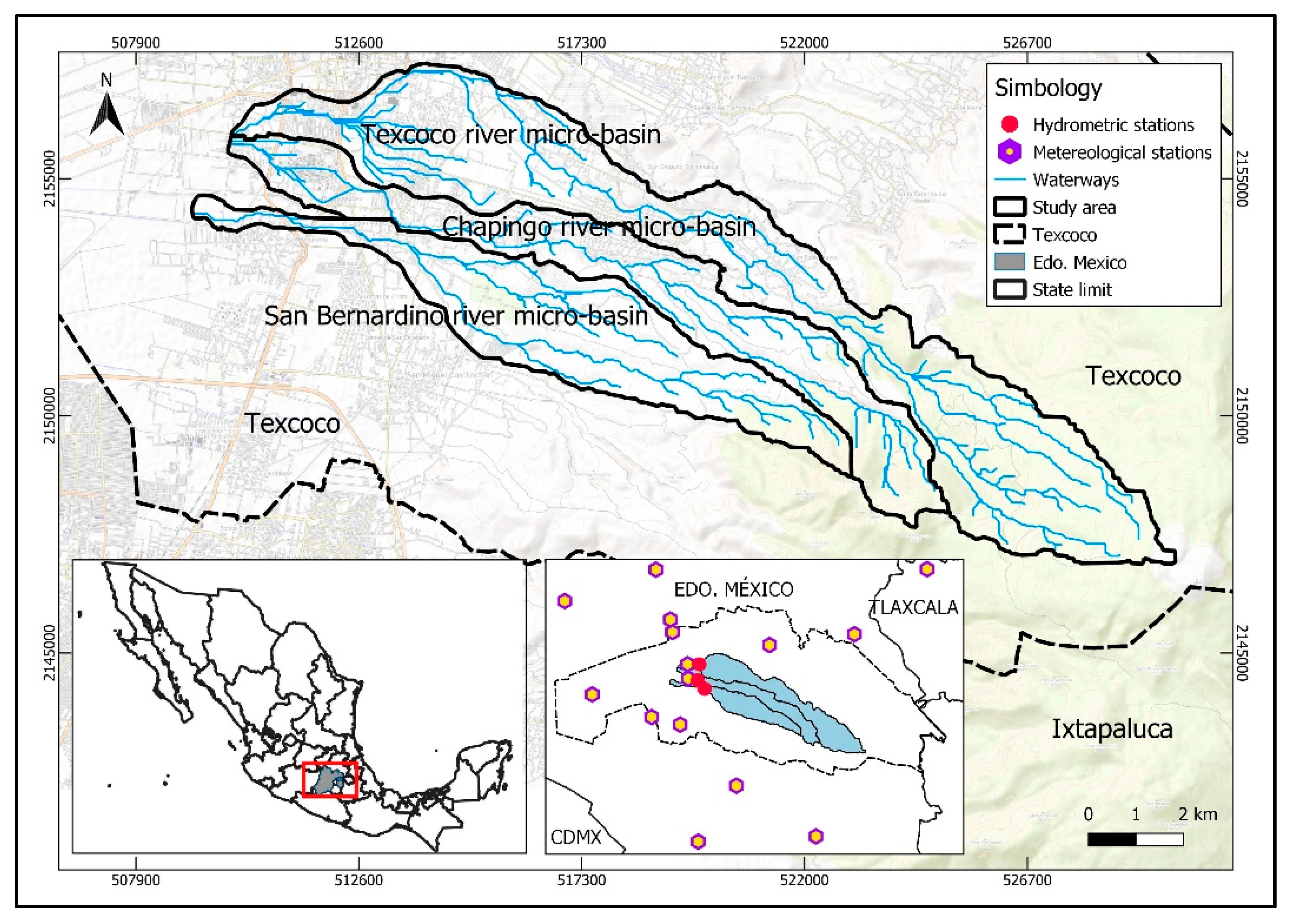
2.1. Study Area

The research was carried out in the three microbasins of the Texcoco, Chapingo, and San Bernardino Rivers in the municipality of Texcoco, Mexico. They are located between the 19°24′ and 19°28′ N parallels and the 98°43′ and 98°52′ W meridians. They are located at an altitude that ranges from 2243 to 4080 m asl and cover a total area of 77.40 km2. These microwatersheds are part of the Texcoco aquifer, key 1507, which belongs to the Pánuco Hydrological Region, within the Hydrological-Administrative Region XIII, Aguas del Valle de México (Figure 1); the aquifer has been reported as being overexploited, and despite the fact that it is completely prohibited by national decrees, said regulatory instruments have not been sufficient to reverse problems related to overexploitation since there is a great demand for groundwater, mainly for urban public use in the region [30]. The temperature ranges between 5 and 16 °C, and the average temperature is 11 °C. Precipitation ranges between 500 and 800 mm per year, with an annual average of 652.5 mm. The predominant climate is temperate dry with cool and rainy summers, with thermal oscillation, interannual Ganges-type temperature variation, and the presence of heat waves (C(w0)bi’gw’’). There is also a semiarid climate with rainy summers (BS1w(w)ki’gw’’) that comprises 21.3% of the total area [31].
The riverbeds in the study area experience ephemeral and intermittent runoff of a torrential nature, with short-term floods and dry streams during the dry season. The three riverbeds, in addition to rainwater, receive and conduct sewage, a situation by which, in many cases, they form parts of the drainage systems [30]. Sedimentary breccia rocks have the greatest distribution, and extrusive igneous rocks of the andesite type are abundant [32]. Hydrogeology indicates that the study area has a medium to high permeability [33]. The soil type with the greatest distribution is epipetric Phaeozem, followed by the epipetroduric Phaeozem [34]. The main types of land use and vegetation correspond to rainfed agriculture (29.6%), temperate forest (26.1%), and reforestation areas (14.8%). In the microbasins of the Texcoco River and Chapingo River, the land uses with the greatest surface areas are temperate forest and vegetation, at 37% and 24.2%, respectively. In the San Bernardino River microbasin, rainfed agriculture is the main land use, at 44.2% (Table 1).

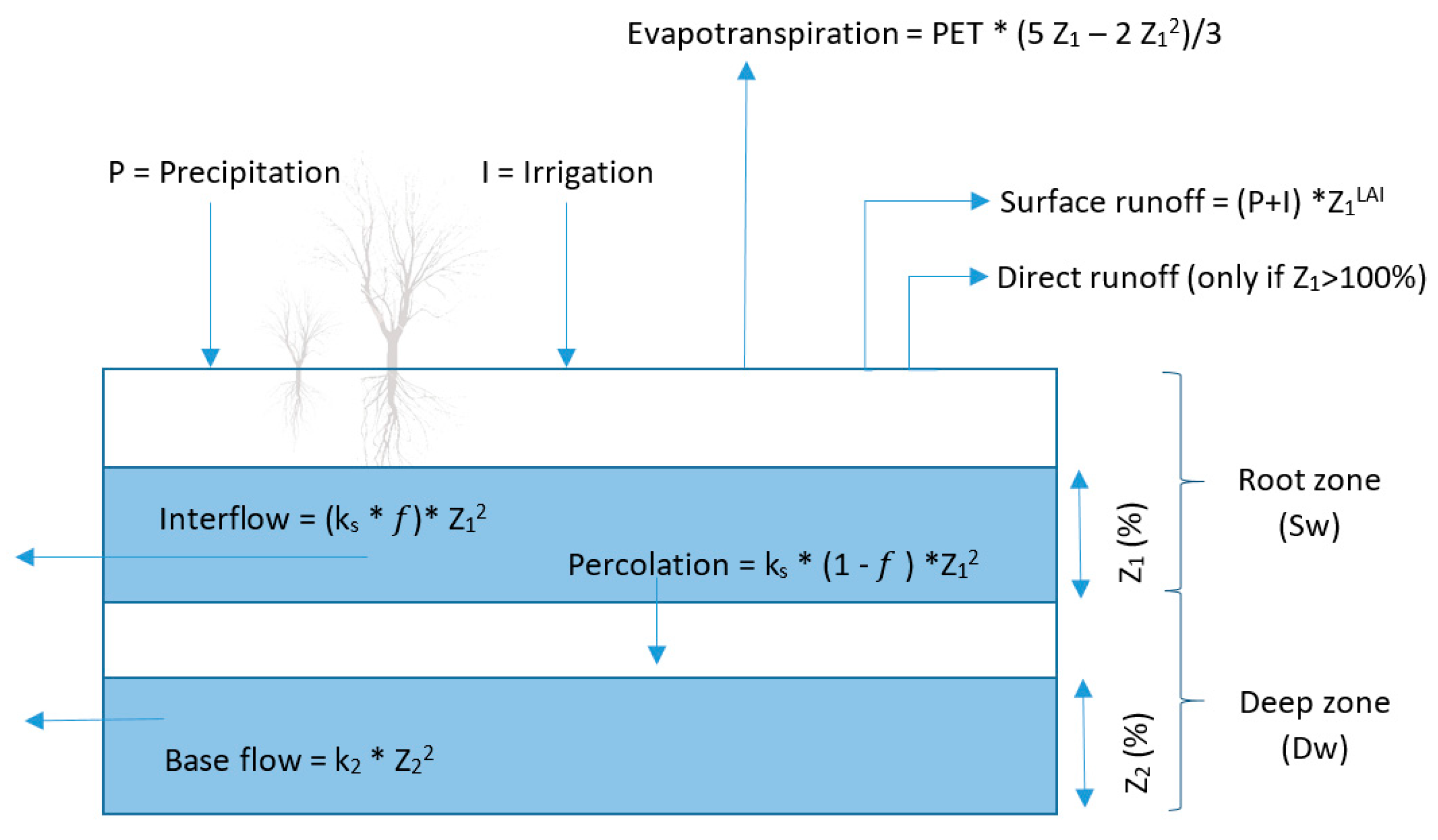
2.2. Hydrological Simulation

To perform hydrological simulations, the WEAP used five methods. In this research, the rain runoff method (soil moisture method) was applied, which represents the basin through two soil layers: the root zone and deep zone (Figure 2). This method characterizes the vegetation cover and soil type, and through specific functions, the processes of evapotranspiration, surface runoff, subsurface runoff, percolation, and base flow are estimated [22,27,35]. The calculation of the hydrological model in the root zone and in the deep zone can be calculated with Equations (1) and (2) [27]. First,
S W j d z i , j d t = P e ( t ) P E T ( t ) K c j ( t ) ( 5 z 1 , j 2 z 1 , j 2 3 ) P e ( t ) z 1 , j L A I j 2 f j k s z 1 , j 2 ( 1 f j ) k j z 1 , j 2
where the 1st term is the changes in the soil moisture; the 2nd factor is the effective precipitation (including irrigation); the 3rd term calculates the evapotranspiration; the 4th factor represents the surface runoff; the 5th term is the intermediate flow; and the 6th term represents percolation. Second,
D W j d z 2 , j d t = ( 1 f j ) k j z 1 , j 2 k 2 z 2 , j 2
where the 1st term is the base flow, and the 2nd term is the percolation.

2.3. Data and Sources of Information

The monthly precipitation and the minimum and maximum temperature data from 15 nearby stations with at least 20 years of information were downloaded from the national database [36] (see Supplementary Materials: Table S1). Isotherms and isohyets were plotted according to the method of Gómez et al. [37]. Relative humidity and wind were averaged monthly, and the WEAP model was fed according to the location of the microwatersheds. The information was obtained from Gómez and Monterroso [38].

2.3.1. Hydrological Catchment Units

The subbasins were subdivided to the determine the value of the flow at a given time during the application of the model more precisely, either for calibration or for the simulation of the scenarios [24]. Following the method of Young et al. [39], the catchments were delimited using the QGIS software through the intersection of the microbasin maps and contour lines at 250 meters. The resulting catchment map was intersected with the land use and vegetation layer (map obtained in the estimation of land use changes) to specify the distribution of the different land use and vegetation types by hydrological unit. In total, 22 catchments were delimited, nine of which belonged to the Texcoco River microbasin, seven of which belonged to the Chapingo River, and six of which belonged to the San Bernardino River (see Supplementary Materials: Figure S1. Location of the Catchments).

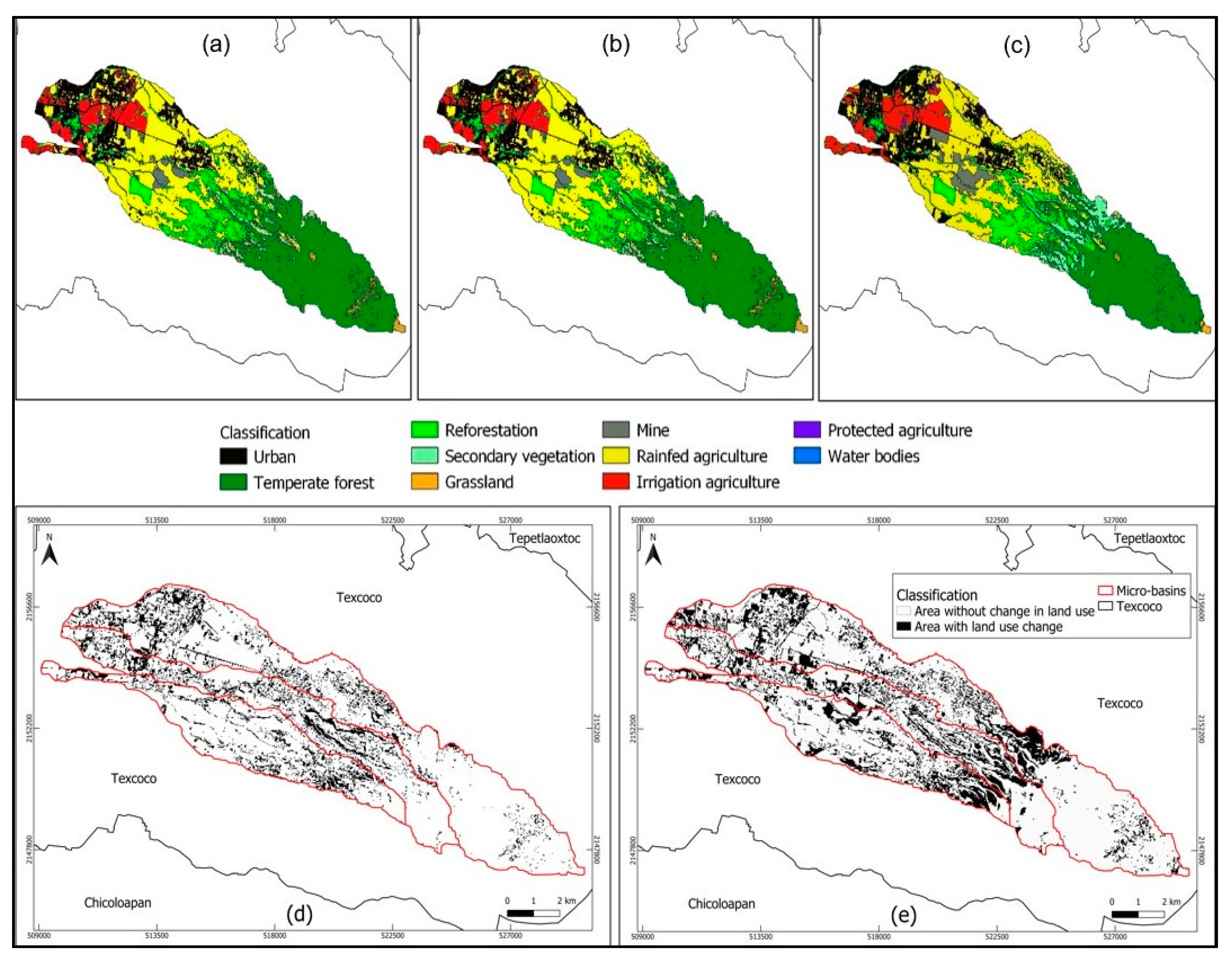
2.3.2. Land Use Changes

Land use changes were estimated through a supervised classification using the GIS data in QGIS and the Semi-Automatic Classification Plugin (SCP) [40]. The supervised classification was based on the Normalized Difference Vegetation Index (NDVI), which highlights certain properties and allows for the spectral behavior of the forest vegetation and the soil to be differentiated. The NVDI is based on red and near-infrared reflectance, the difference of which increases as the density of green leaves increases and therefore increases with the concentration of canopy chlorophyll; therefore, it is a good indicator of the amount of green vegetation. Although the satellite images belong to the United States Geological Survey, they were downloaded directly from the SCP complement and corresponded to the following dates: 28 February 1995 (Landsat 5), 22 May 2008 (Landsat 5), and 23 March 2021 (Landsat 8). They had a spatial resolution of 30 meters per pixel and a percentage of cloudiness that was less than 20%. The original images were preprocessed starting with an assembly of false color bands: 4, 3, and 2 for the Landsat 5 images and 4 and 3 for the Landsat 8 image. The preprocessed images were used as the input data for the classification.
Ten classes of land cover were defined: urban (U), which includes buildings, streets, highways, and unused land; temperate forest (BT); reforestation (R), which refers to preferably deforested or degraded forest areas, where forest trees have been established by planting to recover forest cover; secondary vegetation (VS); grassland (P); mine (M); rainfed agriculture (AT); and irrigated agriculture (AR); protected agriculture (PA); and water bodies (CU). For each of the classes, at least 10 survey polygons were drawn manually. The supervised classification was performed with the c random forest classification complement [40], which is based on an algorithm that begins with a random selection of the predictor variables and results in a collection of identically tree-structured, independent, and distributed classifiers. Each individual tree casts a unitary vote for the most popular class, while the results of the classification are determined from the majority of the votes of each class [41]. The confidence of the results was analyzed through the evaluation report, and some errors were identified and corrected. With the maps obtained, the occupied area was estimated, and then the area that presented some type of land use change in two periods between 1995–2008 and 2008–2021 was determined (Figure 3). A land cover change tool that compares two classifications was applied to evaluate the changes in land cover. A confusion matrix was filled out to determine the changes in land use class as well as permanence.

2.3.3. Hydrological Parameters

The soil moisture method considers the root zone and the deep zone for the calculation of the hydrological balance [24]. The first includes six parameters: water storage capacity in the root zone (Sw), root zone conductivity (Ks), preferential flow direction (f), initial moisture of the upper layer (Z1), coefficient of crop (Kc), and leaf area index (LAI). The deep zone includes three parameters: water storage capacity in the deep zone (Dw), conductivity of the deep layer (Kd), and initial moisture of the lower layer (Z2). In The Supplementary Materials (Table S2), the initial values used for these parameters are shown.

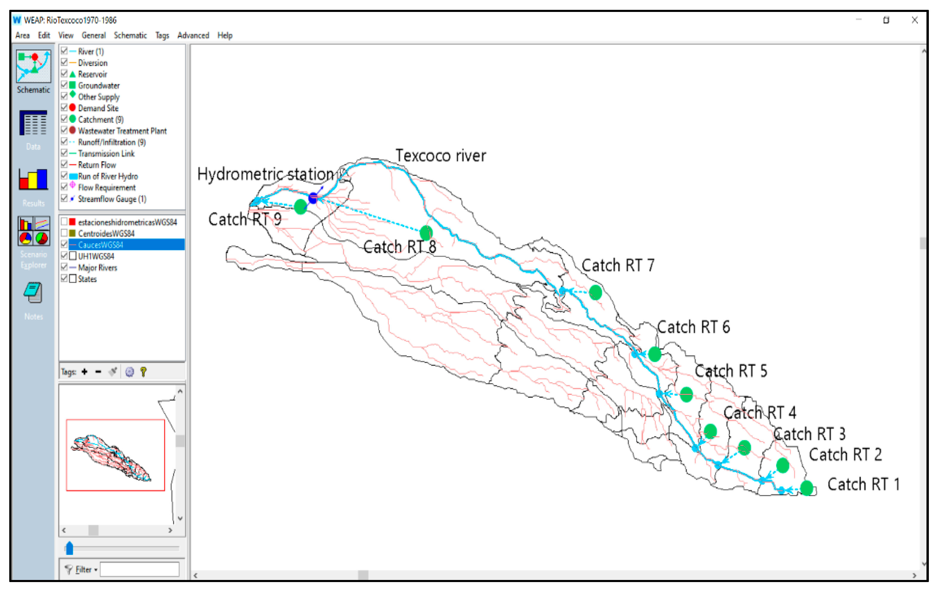
2.4. Model Construction

In the WEAP platform, the following information was added: maps of the microwatersheds, riverbeds, and hydrometric stations and the centroid of the hydrological catchment units. The catchment units were used to establish the locations of the elements of the base scheme: river, hydrological unit, runoff/infiltration lines, and flow meter (Figure 4). The data structure within the catchments included the types of land use and vegetation and climate data. The values of the parameters used to calculate the water balance (Dw, Sw, f, Ks, Kd, Z1, Z2, Kc, LAI) were incorporated into the model using the Key Assumptions tool [42]. The parameters belonging to the upper soil zone were subdivided to incorporate a specific value for each type of land use and vegetation, while in the deep zone parameters, a single value per microbasin was used [42].

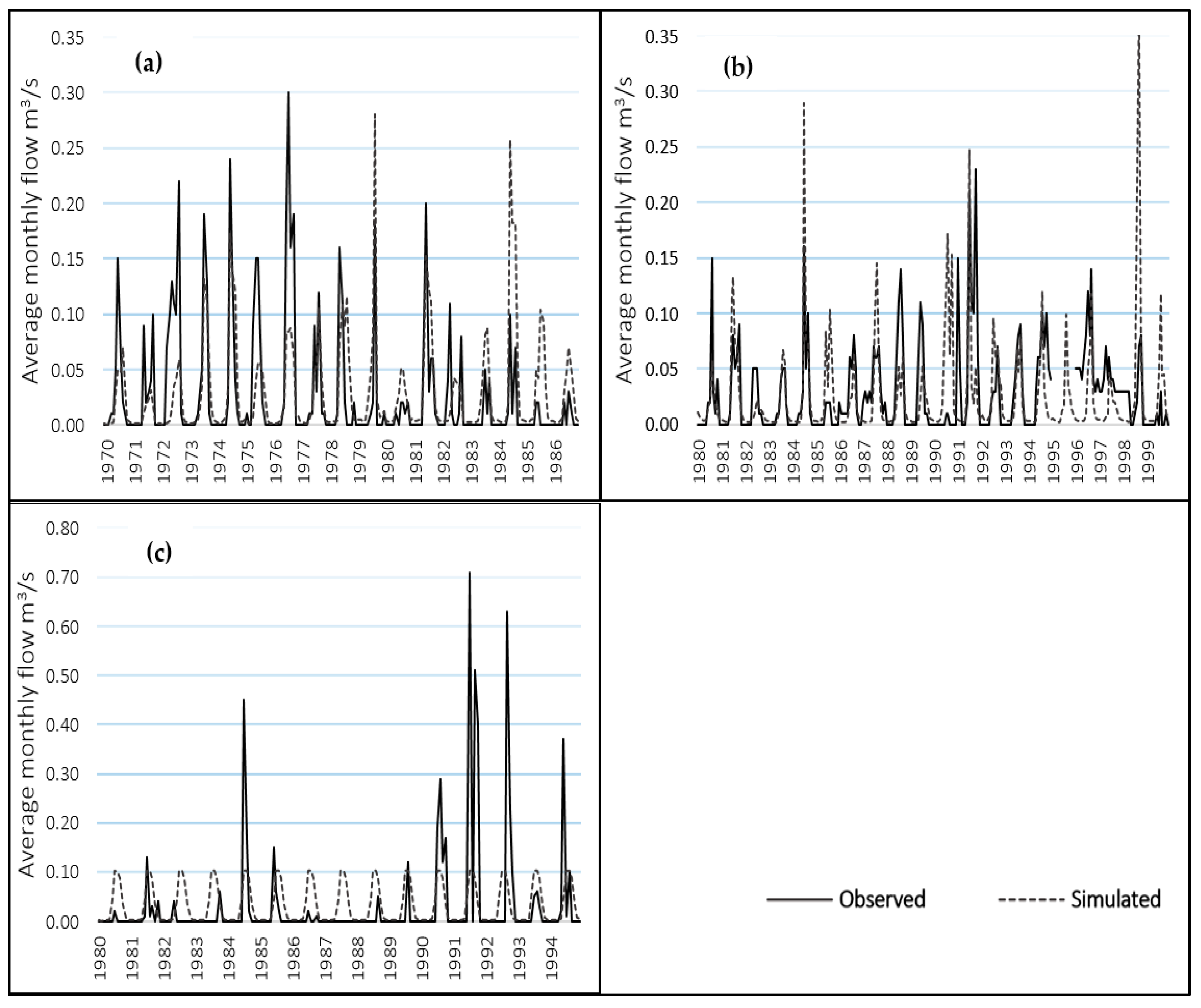
2.5. Calibration and Validation

The model was calibrated with information from the period of 1970–1999 and was based on the coincidence between the historical series of precipitation [36] and the time series of the flow measurement data. The latter were taken from the National Data Bank of Surface Waters (BANDAS) database [43]. The calibration period was 1980–1999 for the Chapingo River, 1980–1994 for the San Bernardino River, and 1970–1986 for the Texcoco River. These periods were selected because of the continuity in their data, and their extension provided variability in the climatic parameters (wet periods and dry periods). The temporal scale of the model was monthly because this was sufficient for the purposes of applying the model, along with the fact that much of the climate data was in this format.
In the calibration of hydrological balance parameters, the sensitivity analysis proposed by Jantzen et al. [44] mentions that the model is highly sensitive to the climate and land use parameters: precipitation, area, Dw, Kc, and LAI (Table 2). The parameters Dw, Kd, Sw, f, Z1, and Z2 were calibrated using the PEST tool, which automates the process of comparing the WEAP results with historical observations and modifying the parameters of the model to improve its accuracy [45].
The validation involved running the model using the values of the parameters that were determined during the calibration process to evaluate the predictive capacity of the model outside of the calibration period [46]. The validation period was 2001–2014 for the Chapingo River, 2001–2003 for the San Bernardino River, and 2011–2014 for the Texcoco River. As in the calibration process, the fit of the model was evaluated graphically and statistically with the measurement of the goodness of fit using the same estimators.

Measurement of Goodness of Fit

Lu and Chiang [47] mentioned that after the sensitivity analysis, the selection of the calibrated ranges and adjusted parameter values are identified based on the statistical criteria: (i) R2, the coefficient of determination, represents the linear correlation between the simulated and observed data. When the value of R2 is close to 1, it indicates a greater correlation. (ii) The Nash–Sutcliffe efficiency (NSE) represents the residuals of the measured data, and its value varies from −ꝏ to 1. An NSE value equal to 1 indicates that the simulation is the same as the observation, while an NSE > 0.5 is an acceptable value for the performance of a model [48]. (iii) Percentage bias (PBIAS) indicates whether the simulated data are overestimated or underestimated. When the PBIAS is greater than 0, the simulation is underestimated, and when the value is less than 0, the simulation is overestimated [49]. (iv) The ratio of the root mean square error to the standard deviation of the observations (RSR), which is defined as the ratio between the mean square error and the standard deviation. The smaller the RSR is, the better the simulation performance is [50]. The goodness of fit of the model was calculated using the RStudio program with the hydroGOF library [51]. The reference values that were used are shown in the Supplementary Materials (Table S3).
Table 2. Parameters, resolution, and sensitivity of land use and climatological variables.
ParametersAbbreviationResolutionSensitivity *
AreaALand useHigh
Water storage capacity in the deep zoneDwBasinHigh
Deep layer conductivityKdBasinModerate
Initial moisture of the lower layerZ2BasinNo influence
Water storage capacity in the root zoneSwSoil typeModerate
Root zone conductivityKsSoil typeModerate
Preferential flow directionfSoil typeModerate
Initial moisture of the upper layerZ1Soil typeNo influence
Crop coefficientKcLand useHigh
Leaf area indexLAILand useHigh
PrecipitationPBasinHigh
TemperatureTBasinModerate
WindVBasinLow
Relative humidityHRBasinLow
LatitudeLBasinLow
Cloud fractionFNBasinLow
* Sensitivity is the influence of a parameter (model input) on the rate of change of the model outputs [52]. It allows us to identify the key parameters and their required precision in the calibration [53].

2.6. Construction of Scenarios

The scenario design was carried out by considering that the main cause of land use change is the high frequency of forest fires. Forest fire events have occurred every five years, with magnitudes ranging between 200 and 300 hectares of affectation. Thus, three scenarios were designed (Table 3), two of which are projected to the year 2047 since this time span is the same number of years over which the land use changes were evaluated (26 years, between 1995 and 2021).
Scenario 1 was called the current scenario and refers to 2021. It incorporates the land use trends observed in the period of 1995–2021. Scenario 2 assumed that there would be no forest fires, that there would be a considerable ecosystem restoration, both by reforestation and by natural regeneration, and that there would be a decline in the agricultural surface. Therefore, it was called a positive trend scenario and was projected to 2047. Scenario 3 considered the ensuing situation of forest fires affecting between 200 and 300 hectares continuing to occur every five years. These fires would not allow the establishment of new reforestation or the natural regeneration of the forest. Considerable advances in agricultural areas would be expected to replace forested areas. Therefore, it was determined to be the negative scenario and was projected to be the scenario representing 2047. The last two scenarios included the new surface values of the land covered by each of the land use and vegetation classes.

2.7. Hydrological Balance

The scenarios were used to determine the hydrological balances in the microwatersheds. In the current scenario, the inputs (precipitation, water stored in the soil from the previous year) and the output flows (evapotranspiration, water storage in the soil, base flow, interflow, surface runoff) were analyzed. Then, land uses were replaced according to the scenario to identify the impact of these land use changes at the microwatershed level on the water balance. In this way, it was possible to quantify how these changes would influence the availability of hydrological environmental services.

3. Results and Discussion

3.1. Changes in Land Use

We must know the historical and current trends that can be observed in the spatiotemporal fluctuation of the changes in the surface of the dominant cover classes [54] to determine the effects that these changes will have on the behavior of the hydrological environmental service balance. The results of the supervised classifications for 1995, 2008, and 2021 are shown in Figure 3. In the period of 1995–2008, the land use changed in 1246 ha, which represents 16% of the total area (Figure 3d). For the period of 2008–2021, changes in land use affected 1906 ha, representing 24% of the total area (Figure 3e). Between 1995 and 2008, the area of temperate forest decreased by 57.6 ha, but in the period of 2008–2021, 323.9 ha were lost, and the sum of the changes in both periods amounted to a decrease of 16.3% (Table 4), mainly because the surface of the lower temperate forest was affected by two forest fires that occurred in 2012 and 2017 [55,56] (see Supplementary Materials: Figure S2). The changes in land use as a consequence of a high frequency of forest fires coincide with the results of [57]. Highly severe forest fires have the potential to interrupt a wide variety of hydrological processes and functions in forested watersheds, such as interception, infiltration, evapotranspiration, and storage [58,59], and their effects can result in an increase in surface runoff and erosion and an increase in the sediment on the riverbeds [60,61,62].
Due to the degradation of the temperate forest by fires, the secondary vegetation showed an increase of 301.7 ha between 1995–2021 (Table 4) since it can sprout quickly after a fire, and if fires are frequent, this type of vegetation can thrive for a long time, and it is unlikely to be successfully replaced [63]. A strong incidence of forest fires has led to forest areas in Mexico where secondary vegetation predominates [64,65].
There was a positive response in the recovery of the degraded area, with a total increase of 184.2 ha for reforestation areas, which will greatly encourage the infiltration levels to be much higher since by reducing surface runoff, the infiltration capacity of rain within the mineral soil will increase [66,67].
Table 5 shows the dynamics of the land use classes. In the of period 1995–2008, the temperate forest changed to reforestation and secondary vegetation at amounts totaling 32.6 and 49.3 ha, respectively, and the reforestation areas mainly changed to secondary vegetation and rainfed agriculture at the amounts of 100.2 and 49.3 hectares, respectively. For the period of 2008–2021, 280.9 ha of the temperate forest changed to secondary vegetation, and 131.5 ha of it changed to reforestation areas. The microwatershed results are presented in the Supplementary Materials (Tables S4 and S5).

3.2. Future Land Use Scenarios

Land use scenarios can consider the aspects of changes in vegetation cover created by future trends such as decreases or increases in forest areas or changes in the types of crops due to economic trends. All of these considerations should be studied so that when modeling the scenario, it is clearly known which variables and functions will be taken into account when defining the scenario [24]. Table 6 shows the percentages of the land cover surfaces with which the proposed scenarios were designed and projected, taking the area percentages of the land use classes in 1995 and 2008 as a reference. Scenario 1 (Current_2021) mainly consists of 2021.4 ha of temperate forest, which is equivalent to 26% of the total area, with 1145.6 ha of reforestation, which corresponds to 14.9% and 2294.8 ha of rainfed agriculture land, which continues to be the land use with the most coverage, even after it decreased by 235.2 ha (most of which become urban areas). Scenario 2 (Positive_2047) is projected to have the largest area of temperate forest (3757 ha), which is equivalent to 48.5% of the total area, with 743 ha of reforestation (9.6%), and with 18.2% of the surface being rainfed agriculture. Scenario 3 (Negative_2047) is projected to have the smallest forest area, and its coverage would only cover 13.6% of the total area (1050 ha), but it would have the highest percentage of urban areas (16.3%) and 3767 ha of rainfed agriculture, which is equivalent to 48.7% of the total area. The Supplementary Materials (Table S6) present additional information on the evolution of land uses.

3.3. Model Calibration

Arnold et al. [46] said that calibration is an effort to better parameterize a model for a given set of local conditions, thus reducing the uncertainty of the prediction. Droogers and Immerzeel [21] held that calibration can be considered parameter estimation or, more generally, an optimization.
Texcoco River: Figure 5a compares the average monthly flow data observed and those simulated by the model. According to the goodness of fit, the model is very good at predicting the hydrological response of the watershed (estimators NSE = 0.98, R2 = 0.93, RSR = 0.15, PBIAS = 5.3). The model fails to simulate the peak flow rates, and the simulated rates are closer to the base flow rates. This behavior of the model differs from the results presented by Ingol-Blanco and McKinney [68], who reported that WEAP better simulates the peak runoff of the base flows in the Conchos River basin.
Chapingo River: In the microbasin, the goodness of fit indicates that the model has a very good ability to predict the hydrological response of the microbasin (NSE = 0.93, R2 = 0.81, RSR = 0.26). The simulation overestimates the flow due to its PBIAS of −13.1 since in most years, the peak flows that are predicted are above those observed. However, this percentage is considered good, and the simulated curves of the base flows are observed closer to the records reported in this period (Figure 5b).
San Bernardino River: In this microwatershed, the goodness of fit indicates that our model is very good (NSE = 0.84, R2 = 0.76, RSR = 0.38) and good according to the PBIAS of −13.5. The simulated flow shows cyclical behavior because the WEAP program allows the calculation to be performed even when there are no precipitation records in a given time. This is possible because WEAP provides the ability to model the flow with full accuracy if the data are available or to calculate them if they are not available [69]. When the precipitation data entered are the values that were calculated using isohyets, then the model fails to simulate the variations in the peak flows, and the simulation is closer to the variation in the base flows (Figure 5c).
Goodness of fit. According to the criteria set by Moriasi et al. [52], the ranges of calibration values are generally classified as being very good by all four estimators, which indicates that the model correctly simulates the hydrological responses of the three microwatersheds. Previous studies have confirmed the capacity of the WEAP model to reproduce the hydrological processes of hydrographic basins in different parts of the world. Among these is the study conducted by Abera Abdi and Ayenew [70], who reported R2, NSE, and RSR values of 0.82, 0.8, and 0.44, respectively. Asghar et al. [71] calibrated their model with an NSE and R2 of 0.85 and 0.86, respectively. Al-Mukhtar and Mutar [72] reported values of R2 and PBIAS during the calibration of 0.70 and 2.52%, respectively. Nevárez et al. [73] obtained values of 0.84, 0.73, and −15.92 for the R2, NSE, and PBIAS estimators, respectively. The validation information and the goodness of fit of the validation are presented in the Supplementary Materials (Figure S3).

3.4. Hydrological Balance

The evaluation of the water resources in a basin requires a correct estimation of the hydrological balance, that is, understanding the cycle in its different phases: the way in which the water that is received from precipitation or mist is distributed between the evapotranspiration process, runoff, and infiltration [74].
The effects of current and evolutionary trends in the land use changes of the temperate forest cover on the hydrological balance were analyzed by evaluating the behavior of the inflow (precipitation, water stored in the forest in the previous year) and the outflows (evapotranspiration, water storage in the soil, base flow, interflow, surface runoff) of the hydrological balance emitted by the model. The flows were taken as indicators to determine how the hydrological resources were distributed in the microwatersheds of the study area. The values were compared to the historical reference data to obtain the percentage change or evolution (Ev%) under the conditions of the projected scenarios in 2021 and 2047 (Table 7).

3.4.1. Current Hydrological Balance

The results of Scenario 1 (Current_2021) indicate that the decrease in the the temperate forest cover (−15.9%) from 2008 as a result of a frequent incidence of forest fires influenced the increase in the surface runoff in the three microwatersheds: 4.2%, 5.3%, and 5.6%. Thus, the microbasin of the San Bernardino River (smallest of the three microbasins studied) presents the greatest increase in runoff at present, in line with the fact that it only has 5.5% temperate forest. coverage There was also an increase of 153.3% in the base flow in the Chapingo River, 412.5% in the Texcoco River, and 154.5% in the San Bernardino River. This increase is related to the increase in the reforestation areas (18.3%) estimated for this scenario. It is worth mentioning reforestation takes more than 5 years, which is the minimum time necessary for a basin to reach a new equilibrium [75]. Therefore, these changes are compensation for the lost forest area. According to the study by [76], there are increases in the base flow that are related to larger forest cover areas due to greater the infiltration and recharge of the underground storage.

3.4.2. Future Projections

The simulation of the hydrological balance in Scenario 2 (Positive_2047) mainly implies an increase in the temperate forest cover (85.9%) over what it currently covers. The increase assumes that there will be no forest fires with significant effects in the next 26 years, a condition that would allow considerable restoration of the ecosystem through both reforestation and natural regeneration. It assumes a decrease in the rainfed agricultural surfaces (−38.7%) that are near or within the preferably forested areas. The results indicate that under these conditions, a decrease in surface runoff is expected in all three microwatersheds: Chapingo River −32.6%, Texcoco River −38.2%, and San Bernardino River −38.8%. These decreases indicate that there would be lower velocity runoff, a condition that occurs when the surfaces are protected by temperate forest cover [67,77].
The projected inflows suggest that there would be an increase in the previous-year soil water storage of 13.8%, 8.5%, and 41.4% in the three respective microbasins, which would increase the water available for infiltration and for the recharge of aquifers [78]. The highest percentages of base flow occur in this scenario: 520% in the Chapingo River, 1250% in the Texcoco River, and 518% in the San Bernardino River microbasin. The increase in base flow corroborates the studies by Price and Jackson [79] and Price et al. [76], who evaluated the base flow of 30 streams in the highlands of the Appalachians, and their results indicate a positive relationship between the forest coverage of the basin and the discharge of the base flow. Increases in the evapotranspiration of 0.7%, 1.2%, and 2.6% would also be expected, and the latter outflow is directly related to the increase in forest cover [80]. However, according to the study reported by Qiu et al. [81], although the increase in forest cover, which is mainly due to the establishment of reforestation, has positive responses with the increase in humidity in the superficial layer of the soil, in the subsoil and in the deep layers of the soil, they led to a significant reduction in the humidity; this negative effect is due to the fact that large-scale restorations consume much more water from the deep soil than natural regeneration; therefore, it will be difficult for local precipitation to replenish the decrease in humidity in the deep zones, and, in turn, this will have negative effects on plant growth and water resources.
The hydrological balance scenario, Scenario 3 (Negative_2047) assumes a 50.1% decrease in temperate forest cover due to the persistence of highly severe forest fires that would result in an 81.7% decrease in reforestation, preventing the establishment of the natural regeneration of the forest. Therefore, in degraded areas, there would be a considerable advance in rainfed agricultural areas (64.2%), which would take the place of what would preferably be forested areas. Under these conditions, the model indicates that surface runoff would increase [54,57] in the three microbasins: Chapingo River (68.2%), Texcoco River (85.4%), and San Bernardino River (49.9%). The elimination of vegetation cover and soil organic matter will lead to changes in the hydrological processes by reducing the interception of precipitation and modifying the structure of the surface soil [14,15,82]. The microbasin of the Texcoco River presents the greatest increase in surface runoff because it would be the one with the greatest loss of forest (687.5 ha). A decrease in the water stored in the soil from the previous year of 32.9%, 2.5%, and 25.3%, respectively, would be expected. The alteration of these flows indicates that the water that is available for hydrological environmental services for the recharge of aquifers will be compromised throughout the study area [83].
The decrease in evapotranspiration of 6.5% in the Chapingo River microbasin, 3.6% in the Texcoco River, and 4.8% in the San Bernardino River is also related to the alteration of the hydrological balance [57,84]. The results coincide with the effects of land use changes on the hydrological components in the Chongwe River basin presented by Tena et al. [85], showing that the actual annual evapotranspiration decreased from 840.6 mm to 796.3 mm due to a decrease of 41.11% in forest cover.

3.4.3. Environmental Hydrological Service in Temperate Forests

The analysis of the hydrological balance according to the catchment groupings where the temperate forest predominates allowed us to more clearly identify the variations in and the distribution of the inflow and outflow of the hydrological balance in the three microbasins related to the changes in the temperate forest cover. Table 8 shows the distributions of the inflow and outflow of the hydrological balance by microbasin as well as the percentage of the evolution (Ev%) of the change in the flows under the three proposed scenarios. The percentage of evolution was generated based on the flows that existed in the reference scenario.
In the inflow of the three microwatersheds, the decrease in the water stored in the soil in the previous year under the conditions of Scenario 3 (negative) stands out at −20.9% in the microwatershed of the Chapingo River, −13.3% in the Texcoco River, and −34.2% in the San Bernardino River because changes in the soil cover strongly affect the distribution of soil moisture and the hydraulic properties of the soil [86,87]. In all of the outflows of the scenarios of the three microwatersheds, there is variation in the distribution of water resources, but the decrease in water storage in the soil stands out: −15.1% in the Chapingo River, −12.3% in the Texcoco River, and −27% in the San Bernardino River. The capacity of the soil to store and regulate the flow of water largely depends on its infiltration rate and depth, but disturbances such as changes in land use and fires can alter these soil capacities [88]. These alterations are caused because without forest cover to protect the soil, the soil is exposed to intense rainfall that can cause water erosion, compaction [89], and alterations in their structure (higher apparent density, lower field capacity, disappearance of organic matter and microfauna) [88]. The decrease in soil moisture coincides with the statistical results of a study along the karst slopes of Southwest China, which showed that changes in soil cover strongly affect the distribution of soil moisture. When compared to bare soil areas, the forest, shrub, and grass areas had 30.5, 20.1, and 10.2% higher soil moisture values, respectively [86].
Regarding the evolution of the changes that the surface runoff presents and would present, it can be observed that currently (Scenario 1), this flow has increased by 57.1% in the Chapingo River, 35.9% in the Texcoco River, and 172.2% in the San Bernardino River microwatersheds. However, under the conditions of the negative scenario, it is expected that surface runoff will increase 346.3% in the Chapingo River, 287.4% in the Texcoco River, and 729.6% in the San Bernardino River. These values would decrease under the conditions of Scenario 2 (positive): −45.2%, −49.6%, and −49.8%, respectively. The decrease in surface runoff is directly associated with the rain that is intercepted by the canopy because it is an important process in the water balance of forests [90]. The temperate forest canopy is also an important factor for soil conservation due to its role in reducing the erosive impact of rainfall [91]. Another factor that influences the reduction of surface runoff is the incorporation of organic matter into the soil by the temperate forest since its presence at high values reduces the risks of soil water erosion [92] and promotes water infiltration to the root zone and the deep zone. Therefore, the hydrological functions, as highlighted by Esse et al. [93], are more efficient in watersheds with forest cover and that are made up of native or exotic species than in agricultural cover basins with annual crop rotations.

4. Conclusions

In the study area, the temperate forest land area decreased by 16% from 1995–2021. The incidence of forest fires has been an important cause of this decrease. The presence of secondary vegetation is an indicator of the degradation and recovery of the ecosystem, as it can sprout quickly after a forest fire. Changes in land use and the presence of forest fires are included in the WEAP software to measure the hydrological response of watersheds. The WEAP model is a tool that can be incorporated into the forestry sector to determine the current and future behavior of hydrological resources and to support decision-making for the integral management and valuation of hydrological environmental services. Doing so would ensure the integral, continuous, and stable flow of environmental services provided by temperate forests.
The effect of maintaining a healthy forest without forest fires translates into lesser surface runoff, lower runoff velocity, and more water being available in the soil for infiltration and aquifer recharge. That is, it maintains the hydrological environmental service. Forest fires reduce rain interception and increase the velocity and flow of surface runoff, which modify the structure and composition of soils, thereby compromising hydrological environmental services. New studies are suggested to investigate the modifications of the water balance during forest fires.

Supplementary Materials

The following are available online at https://www.mdpi.com/article/10.3390/w14030383/s1, Table S1: Data and location of meteorological stations, Figure S1: Location of the catchments, Table S2: Initial values of the parameters of the soil moisture method); the initial values used for these parameters are shown, Table S3: Range of values for the interpretation of the goodness of fit estimators, Figure S2: Location of the areas affected by forest fires, Tables S4 and S5: Dynamics of land use changes by microbasin in the periods of 1995–2008 and 2008–2021, Table S6: Evolution of land use changes according to the projection of scenarios, Figure S3: Average monthly flow simulated and observed in the validation periods.

Author Contributions

Conceptualization, V.H.R.-G., J.D.G.-D. and A.I.M.-R.; methodology, V.H.R.-G., J.D.G.-D., C.A.-G. and A.I.M.-R.; software, V.H.R.-G.; validation, V.H.R.-G., J.D.G.-D., C.A.-G. and A.I.M.-R.; formal analysis, V.H.R.-G., M.A.B.d.l.R., J.D.G.-D., C.A.-G., M.M.-R. and A.I.M.-R.; investigation, V.H.R.-G.; resources, A.I.M.-R.; writing—original draft preparation, V.H.R.-G. and A.I.M.-R.; writing—review and editing, V.H.R.-G., M.A.B.d.l.R., J.D.G.-D., C.A.-G., M.M.-R. and A.I.M.-R.; supervision, M.A.B.d.l.R., J.D.G.-D., C.A.-G., M.M.-R. and A.I.M.-R. All authors have read and agreed to the published version of the manuscript.

Funding

This research received no external funding. V.H.R.G. received a scholarship from the National Council of Science and Technology (CONACYT). The APC was funded by DGIP program by Universidad Autónoma Chapingo.

Institutional Review Board Statement

Not applicable.

Informed Consent Statement

Not applicable.

Data Availability Statement

Data are available upon reasonable request from the corresponding author.

Acknowledgments

Gratitude is extended to the National Council of Science and Technology (CONACYT), to the Universidad Autónoma Chapingo, DGIP, Division of Forest Sciences, as well as the Master of Science Program in Forest Sciences. We gratefully acknowledge the comments and suggestions of the anonymous reviewers, whose comments have substantially improved the paper.

Conflicts of Interest

The authors declare no conflict of interest.

References

  1. Flores-López, F.; Galaitsi, S.; Escobar, M.; Purkey, D. Modeling of Andean Páramo Ecosystems’ Hydrological Response to Environmental Change. Water 2016, 8, 94. [Google Scholar] [CrossRef]
  2. Millennium Ecosystem Assessment. Ecosystems and Human Well-Being: Synthes; Island Press: Washington, DC, USA, 2005; p. 137. [Google Scholar]
  3. Secretaría del Medio Ambiente y Recursos Naturales (Semarnat). Ecosistemas Terrestres. In Informe de la Situación del Medio Ambiente en México 2012; Semarnat: Zapopan, Mexico, 2012; pp. 40–118. [Google Scholar]
  4. Balvanera, P.; Cotler, H.; Aburto, O.; Aguilar, A.; Aguilera, M.; Aluja, M.; Andrade, A.; Arroyo, I.; Ashworth, L.; Astier, M.; et al. Estado y tendencias de los servicios ecosistémicos. In Capital Natural de México, Vol. II: Estado de Conservación y Tendencias de Cambio; Conabio: Tlalpan, Mexico, 2009; pp. 185–245. [Google Scholar]
  5. Roffe, T.G.; Toruño, P.J.; Orantes, E.A.M.; Espinoza, E.I.G. Servicios ambientales y gestión de los recursos hídricos utilizando el modelo WEAP: Casos de estudio en Iberoamérica. Rev. Iberoam. Bioecon. Cambio Clim. 2015, 1, 72–87. [Google Scholar] [CrossRef] [Green Version]
  6. Isik, S.; Kalin, L.; Schoonover, J.E.; Srivastava, P.; Lockaby, B.G. Modeling effects of changing land use/cover on daily streamflow: An Artificial Neural Network and curve number based hybrid approach. J. Hydrol. 2013, 485, 103–112. [Google Scholar] [CrossRef]
  7. Brauman, K.A.; Daily, G.C.; Duarte, T.K.; Mooney, H.A. The nature and value of ecosystem services: An overview highlighting hydrologic services. Ann. Rev. Environ. Resour. 2007, 32, 67–98. [Google Scholar] [CrossRef]
  8. Comisión Nacional del Agua (Conagua). Atlas del Agua en México 2015; Secretaría del Medio Ambiente y Recursos Naturales: Zapopan, Mexico, 2015; p. 135.
  9. Brauman, K.A. Hydrologic ecosystem services: Linking ecohydrologic processes to human well-being in water research and watershed management. WIREs Water 2015, 2, 345–358. [Google Scholar] [CrossRef]
  10. Manson, E. Los servicios hidrológicos y la conservación de los bosques de México. Madera Bosques 2016, 10, 3–20. [Google Scholar] [CrossRef]
  11. De la Maza, H.R. Pago por servicios ambientales México. In Agua: El oro Azul; Senado de la República, LXI Legislatura, Comisión de Recursos Hidráulicos, Comisión de Medio Ambiente, Recursos Naturales y Pesca: Ciudad de México, Mexico, 2012; pp. 73–88. [Google Scholar]
  12. Zilberman, D.; Lipper, L.; McCarthy, N. Putting Payments for Environmental Services in the Context of Economic Development. In Payment for Environmental Services in Agricultural Landscapes; The Food and Agriculture Organization of the United Nations: New York, NY, USA, 2009; pp. 1–25. [Google Scholar]
  13. Rzedowski, J. Capítulo 4: Influencia del hombre. In Vegetación de México, 1st ed.; Comisión Nacional para el Conocimiento y Uso de la Biodiversidad: México D.F., Mexico, 2006; pp. 59–74. [Google Scholar]
  14. Aboelnour, M.; Gitau, M.W.; Engel, B.A. A Comparison of Streamflow and Baseflow Responses to Land-Use Change and the Variation in Climate Parameters Using SWAT. Water 2020, 12, 191. [Google Scholar] [CrossRef] [Green Version]
  15. Khoshnoodmotlagh, S.; Verrelst, J.; Daneshi, A.; Mirzaei, M.; Azadi, H.; Haghighi, M.; Hatamimanesh, M.; Marofi, S. Transboundary basins need more attention: Anthropogenic impacts on land cover changes in aras river basin, monitoring and prediction. Remote Sens. 2020, 12, 3329. [Google Scholar] [CrossRef]
  16. Comisión Nacional Forestal (Conafor). Programas y Acciones en Reforestación, Conservación y Sanidad Forestal de Ecosistemas Forestales; Coordinación General de Conservación y Restauración: Zapopan, Mexico, 2010; p. 108.
  17. Kepner, W.G.; Ramsey, M.M.; Brown, E.S.; Jarchow, M.E.; Dickinson, K.J.M.; Mark, A.F. Hydrologic futures: Using scenario analysis to evaluate impacts of forecasted land use change on hydrologic services. Ecosphere 2012, 3, 1–25. [Google Scholar] [CrossRef]
  18. Vargas, C.R.d.C.; Sanchez, T.G.; Rolón, A.J.C.; Pichardo, R.R.; Tobías, J.R.; Treviño, T.J. Disponibilidad de los Recursos Hídricos ante Escenarios de Cambio Climático en una Cuenca Costera de Tamaulipas, México. Investig. Actuales Medioambiente 2015, 1, 86–100. [Google Scholar]
  19. Abbaspour, K.C.; Yang, J.; Maximov, I.; Siber, R.; Bogner, K.; Mieleitner, J.; Zobrist, J.; & Srinivasan, R. Modelling hydrology and water quality in the pre-alpine/alpine Thur watershed using SWAT. J. Hydrol. 2007, 333, 413–430. [Google Scholar] [CrossRef]
  20. Qiu, L.; Chen, Y.; Wu, Y.; Xue, Q.; Shi, Z.; Lei, X.; Liao, W.; Zhao, F.; Wang, W. The water availability on the Chinese Loess Plateau since the implementation of the grain for green project as indicated by the evaporative stress index. Remote Sens. 2021, 13, 3302. [Google Scholar] [CrossRef]
  21. Droogers, P.; Immerzeel, W.W. Calibration Methodologies in Hydrological Modeling: State of the Art. In National User Support Programme 2001–2005. FutureWater-Science for Solutions; Citeseer: Princeton, NJ, USA, 2006; Volume 9, p. 36. [Google Scholar]
  22. Esquivel, A.G.; Nevarez, F.M.M.; Velásquez, V.M.A.; Sánchez, C.I.; Bueno, H.P. Hydrological modeling of a basin in Mexico’s arid northern region and its response to environmental changes. Agric. Biosyst. Eng. 2017, 9, 3–17. [Google Scholar] [CrossRef] [Green Version]
  23. López, G.T.G.; Manzano, M.G.; Ramírez, A.I. Disponibilidad hídrica bajo escenarios de cambio climático en el Valle de Galeana, Nuevo León, México. Tecnol. Cienc. Agua 2017, 8, 105–114. [Google Scholar] [CrossRef]
  24. Centro de Cambio Global (CCG); Universidad Católica de Chile, Stockholm Environment Institute. Guía Metodológica—Modelación Hidrológica y de Recursos Hídricos con el Modelo WEAP; Boston: Santiago, Chile, 2009; p. 86. [Google Scholar]
  25. Amato, C.; McKinney, D.; Ingol-Blanco, E.; Teasley, R.L. WEAP Hydrology Model Applied: The Rio Conchos Basin; Center for Research in Water Resources, University of Texas at Austin: Austin, TX, USA, 2006; p. 69. [Google Scholar]
  26. Ahmadaali, J.; Barani, G.-A.; Qaderi, K.; Hessari, B. Analysis of the Effects of Water Management Strategies and Climate Change on the Environmental and Agricultural Sustainability of Urmia Lake Basin, Iran. Water 2018, 10, 160. [Google Scholar] [CrossRef] [Green Version]
  27. Yates, D.; Sieber, J.; Purkey, D.; Huber-Lee, A. WEAP21—A demand-, priority-, and preference-driven water planning model. Part 1: Model characteristics. Water Int. 2005, 30, 487–500. [Google Scholar] [CrossRef]
  28. Labrador, A.F.; Zúñiga, J.M.; Romero, J. Desarrollo de un modelo para la planificación integral del recurso hídrico en la cuenca hidrográfica del Río Aipe, Huila, Colombia Development of a model for integral planning of water resources in Aipe catchment, Huila, Colombia. Rev. Ing. Reg. 2016, 15, 23–35. [Google Scholar] [CrossRef] [Green Version]
  29. Liu, T.; Merrill, N.H.; Gold, A.J.; Kellogg, D.Q.; Uchida, E. Modeling the production of multiple ecosystem services from agricultural and forest landscapes in Rhode Island. Agric. Resour. Econ. Rev. 2013, 42, 251–274. [Google Scholar] [CrossRef]
  30. Secretaría de Medio Ambiente y Recursos Naturales (Semarnat). Acuerdo Por el Que se Dan a Conocer los Resultados del Estudio Técnico de las Aguas Nacionales Subterráneas del Acuífero Texcoco, Clave 1507, en el Estado de México, Región Hidrológico-Administrativa XIII, Aguas del Valle de México; Secretaría de Gobernación, Diario Oficial de la Federación (DOF): Ciudad de México, Mexico, 2019; p. 12.
  31. García, E. Modificaciones al Sistema Climático de Köppen para la República Mexicana; Instituto de Geografia, Universidad Autónoma de México (UNAM): Mexico City, Mexico, 2004. [Google Scholar]
  32. Instituto Nacional de Estadística y Geografía (INEGI). Conjunto de Datos Geológicos Vectoriales E1402. Escala 1:250,000. Serie I; INEGI: Aguascalientes, Mexico, 2002.
  33. Universidad Autónoma Chapingo (UNAM). Atlas Nacional de México, Vol II: Hidrogeología, Escala 1:4,000,000; Instituto de Geografía, UNAM: Mexico City, Mexico, 1990. [Google Scholar]
  34. Instituto Nacional de Estadística y Geografía (INEGI). Conjunto de datos Vectorial Edafológico, Escala 1:250,000 Serie II (Conjunto Nacional); INEGI: Aguascalientes, Mexico, 2014.
  35. Sieber, J.; Purkey, D. WEAP Water Evaluation and Planning System User Guide; Stockholm Environment Institute, U.S. Center. E. U.: Somerville, MA, USA, 2015; p. 343. [Google Scholar]
  36. Servicio Metereológico Nacional (SMN). Información Climatológica Nacional: Información de Estaciones Climatológicas; Comisión Nacional del Agua (Conagua): Mexico City, Mexico, 2020.
  37. Gómez, J.D.; Etchevers, J.D.; Monterroso, A.I.; Gay, C.; Campo, J.; Martínez, M. Spatial estimation of mean temperature and precipitation in areas of scarce meteorological information. Atmosfera 2008, 21, 35–56. [Google Scholar]
  38. Gómez-Díaz, J.D.; Monterroso-Rivas, A.I. Actualización de la Delimitación de Las Zonas Áridas, Semiáridas y Sub-Húmedas Secas de México a Escala Regional. Reporte Final de Proyecto de Investigación Fondo CONAFOR-CONACYT; Universidad Autónoma Chapingo, Departamento de Suelos: Texcoco, Mexico, 2012. [Google Scholar]
  39. Young, C.A.; Escobar-Arias, M.I.; Fernandes, M.; Joyce, B.; Kiparsky, M.; Mount, J.F.; Mehta, V.K.; Purkey, D.; Viers, J.H.; Yates, D. Modeling the Hydrology of Climate Change in California’s Sierra Nevada for Subwatershed Scale Adaptation 1. J. Am. Water Resour. Assoc. 2009, 45, 1409–1423. [Google Scholar] [CrossRef]
  40. Congedo, L. Complemento de clasificación semiautomático: Una herramienta de Python para la descarga y el procesamiento de imágenes de detección remota en QGIS. Rev. Softw. Código Abierto 2021, 6, 3172. [Google Scholar] [CrossRef]
  41. Breiman, L. RFRSF: Employee Turnover Prediction Based on Random Forests and Survival Analysis. Random For. 2001, 45, 5–32. [Google Scholar] [CrossRef]
  42. Stockholm Environment Institute (SEI). Water Evaluation and Planning System Tutorial Español; SEI: Somerville, MA, USA, 2017. [Google Scholar]
  43. Comisión Nacional del Agua (Conagua). Banco Nacional de Datos de Aguas Superficiales (BANDAS); Conagua: México City, Mexico, 2016.
  44. Jantzen, T.; Klezendorf, B.; Middleton, J.; Smith, J. WEAP Hydrology Modeling Applied: The Upper Rio Florido Rive Basin; Center for Research in Water Resources; The University of Texas: Austin, TX, USA, 2006. [Google Scholar]
  45. Water Evaluation and Planning System (WEAP). Versión 2021. Windows; Stockholm Environment Institute (SEI): Stockholm, Sweden, 2021.
  46. Arnold, J.G.; Moriasi, D.N.; Gassman, P.W.; Abbaspour, K.C.; White, M.J. SWAT: Model use, calibration, and validation. Trans. ASABE 2012, 55, 1549–1559. [Google Scholar] [CrossRef]
  47. Lu, C.; Chiang, L.-C. Assessment of Sediment Transport Functions with the Modified SWAT-Twn Model for a Taiwanese Small Mountainous Watershed. Water 2019, 11, 1749. [Google Scholar] [CrossRef] [Green Version]
  48. Nash, J.E.; Sutcliffe, I.V. River flow forecasting through conceptual models part I—A discussion of principles. J. Hydrol. 1970, 10, 282–290. [Google Scholar] [CrossRef]
  49. Vijai, H.; Sorooshian, S.; Yapo, P.O. Status of automatic calibration for hydrologic models: Comparison with multilevel expert calibration. J. Hydrol. Eng. 1999, 4, 135–143. [Google Scholar]
  50. Singh, J.; Knapp, H.; Demissie, M. Hydrologic modeling of the Iroquois River watershed using HSPF and SWAT. J. Am. Water Resour. Assoc. 2005, 4030, 343–360. [Google Scholar] [CrossRef]
  51. Zambrano-Bigiarini, M. Goodness-of-fit functions for comparison of simulated and observed hydrological time series. In Package ‘hydroGOF’ March; Universidad de La Frontera: Temuco, Araucanía, Chile, 2020; p. 76. [Google Scholar]
  52. Moriasi, D.N.; Arnold, J.G.; Liew, M.W.V.; Bingner, R.L.; Harmel, R.D.; Veith, T.L. Model evaluation guidelines for systematic quantification of accuracy in watershed simulations. ASABE 2007, 50, 885–900. [Google Scholar] [CrossRef]
  53. Ma, L.; Ascough Ii, J.C.; Ahuja, L.R.; Shaffer, M.J.; Hanson, J.D.; Rojas, K.W. Root zone water quality model sensitivity analysis using Monte Carlo simulation. Trans. ASAE 2000, 43, 883. [Google Scholar] [CrossRef] [Green Version]
  54. Martínez Sifuentes, A.R.; Villanueva-Díaz, J.; Ávalos, J.E.; Vázquez, C.V.; Castillo, I.O. Pérdida de suelo y modificación de escurrimientos causados por el cambio de uso de la tierra en la cuenca del río Conchos, Chihuahua. Nova Sci. 2020, 12, 1–26. [Google Scholar] [CrossRef]
  55. Hernández, V.G.A.; Gutiérrez, C.M.d.C.; Barragan, M.S.M.; Ángeles, C.E.R.; Gutiérrez, C.E.V.; Ortiz, S.C.A. La mineralogía en la estimación de las temperaturas de los incendios forestales y sus efectos inmediatos en Andosoles, Estado de México. Madera Bosques 2020, 26, e2611932. [Google Scholar] [CrossRef]
  56. Protectora de Bosques del Estado de México (Probosque). Estadisticas de Incendios Forestales en el Estado de México: Administrador de Base de Datos PostGIS; Probosque: Mexico City, Mexico, 2021.
  57. León-Muñoz, J.; Aguayo, R.; Marcé, R.; Catalán, N.; Woelfl, S.; Nimptsch, J.; Arismendi, I.; Contreras, C.; Soto, D.; Miranda, A. Climate and Land Cover Trends Affecting Freshwater Inputs to a Fjord in Northwestern Patagonia. Front. Mar. Sci. 2021, 8, 960. [Google Scholar] [CrossRef]
  58. Ebel, B.A.; Moody, J.A. Synthesis of soil-hydraulic properties and infiltration timescales in wildfire-affected soils. Hydrol. Processes 2017, 31, 324–340. [Google Scholar] [CrossRef]
  59. Poon, P.K.; Kinoshita, A.M. Spatial and temporal evapotranspiration trends after wildfire in semi-arid landscapes. J. Hydrol. 2018, 559, 71–83. [Google Scholar] [CrossRef]
  60. Kinoshita, A.M.; Chin, A.; Simon, G.L.; Briles, C.; Hogue, T.S.; O’Dowd, A.P.; Gerlak, A.K.; Albornoz, A.U. Wildfire, water, and society: Toward integrative research in the “Anthropocene”. Anthropocene 2016, 16, 16–27. [Google Scholar] [CrossRef] [Green Version]
  61. Rengers, F.K.L.A.; McGuire, J.W.; Kean, D.M.; Staley, D.E.J.H. Model simulations of flood and debris flow timing in steep catchments after wildfire. Water Resour. Res. 2016, 52, 6041–6061. [Google Scholar] [CrossRef] [Green Version]
  62. Robichaud, P.R.; Wagenbrenner, J.W.; Pierson, F.B.; Spaeth, K.E.; Ashmun, L.E.; & Moffet, C.A. Infiltration and interrill erosion rates after a wildfire in western Montana, USA. Catena 2016, 142, 77–88. [Google Scholar] [CrossRef] [Green Version]
  63. Rzedowski, J. Capítulo 17: Bosque de coníferas. In Vegetación de México, 1st ed.; Comisión Nacional para el Conocimiento y Uso de la Biodiversidad: México D.F., Mexico, 2006; pp. 295–327. [Google Scholar]
  64. Miranda, F.; Hernández, X.E. Los tipos de vegetación de México y su clasificación. Bot. Sci. 2016, 28, 29. [Google Scholar] [CrossRef]
  65. Secretaría del Medio Ambiente y Recursos Naturales (Semarnat). Informe de la Situación del Medio Ambiente en Mexico. In Compendio de Estadísticas Ambientales. Indicadores Clave y de Desempeño Ambiental; Semarnat: Zapopan, Mexico, 2012; p. 361. [Google Scholar]
  66. Laino-Guanes, R.; Suárez-Sánchez, J.; González-Espinosa, M.; Musálem-Castillejos, K.; Ramírez-Marcial, N.; Bello-Mendoza, R.; Jiménez, F. Modelación del balance hídrico y el movimiento de nutrientes utilizando WEAP: Limitaciones para modelar los efectos de la restauración forestal y el cambio climático en la cuenca alta del río Grijalva. Aqua-LAC 2017, 9, 46–58. [Google Scholar] [CrossRef]
  67. Hernández, I.U.; Alfaro, B.R.; Menéndez, M.G.; Becerra, L.W.M.; Garnica, J.G.F.; Torrens, Y.A. Impacto de quemas prescritas en la estabilidad del escurrimiento superficial en un bosque de pino. Madera Bosques 2020, 26, 1–12. [Google Scholar] [CrossRef]
  68. Ingol-Blanco, E.; McKinney, D.C. Development of a hydrological model for the rio Conchos basin. Am. Soc. Civ. Eng. 2013, 18, 340–351. [Google Scholar] [CrossRef]
  69. Kandera, M.; Výleta, R.; Liová, A.; Danáčová, Z.; Lovasová, Ľ. Testing of water evaluation and planning (Weap) model for water resources management in the hron river basin. Acta Hydrol. Slov. 2021, 22, 30–39. [Google Scholar] [CrossRef]
  70. Abdi, D.A.; Ayenew, T. Evaluation of the WEAP model in simulating subbasin hydrology in the Central Rift Valley basin, Ethiopia. Ecol. Processes 2021, 10, 41. [Google Scholar] [CrossRef]
  71. Asghar, A.; Iqbal, J.; Amin, A.; Ribbe, L. Integrated hydrological modeling for assessment of water demand and supply under socio-economic and IPCC climate change scenarios using WEAP in Central Indus Basin. J. Water Supply Res. Technol. AQUA 2019, 68, 136–148. [Google Scholar] [CrossRef] [Green Version]
  72. Al-Mukhtar, M.M.; Mutar, G.S. Modelling of Future Water Use Scenarios Using WEAP Model: A Case Study in Baghdad City, Iraq. Eng. Technol. J. 2020, 39, 488–503. [Google Scholar] [CrossRef]
  73. Nevárez, F.M.M.; Fernández, R.D.S.; Sánchez, C.I.; Sánchez, G.M.; Macedo, C.A.; Palacios, E.C. Comparación de los modelos WEAP y SWAT en una cuenca de Oaxaca. Tecnol. Cienc. Agua 2021, 12, 358–401. [Google Scholar] [CrossRef]
  74. García-Coll, I.; Martínez, A.; Ramírez, A.; Niño, A.; Rivas, J.A.; Domínguez, L. La relación agua-bosque: Delimitación de zonas prioritarias para pago de servicios ambientales hidrológicos en la cuenca del río Gavilanes, Coatepec, Veracruz. In El Manejo Integral de Cuencas en México. Estudios y Reflexiones para Orientar la Política Ambiental, 2nd ed.; Cotler, H., Ed.; Instituto Nacional de Ecología: Ciudad de México, Mexico, 2007; pp. 113–130. [Google Scholar]
  75. Brown, A.E.; Zhang, L.; McMahon, T.A.; Western, A.W.; Vertessy, R.A. A review of paired catchment studies for determining changes in water yield resulting from alterations in vegetation. J. Hydrol. 2005, 310, 28–61. [Google Scholar] [CrossRef]
  76. Price, K.; Jackson, C.R.; Parker, A.J.; Reitan, T.; Dowd, J.; Cyterski, M. Effects of watershed land use and geomorphology on stream low flows during severe drought conditions in the southern Blue Ridge Mountains, Georgia and North Carolina, United States. Water Resour. Res. 2011, 47, W02516. [Google Scholar] [CrossRef]
  77. Viramontes, D.; Descroix, L.; Bollery, A. Variables de suelos determinantes del escurrimiento y la erosión en un sector de la Sierra Madre Occidental. Ing. Hidraul. Mex. 2006, 21, 73–83. [Google Scholar]
  78. Morales, D.; Rostagno, M.; La Manna, L. Impacto del fuego sobre el comportamiento hidrológico del suelo en un bosque de ciprés. Patagon. For. 2010, 1, 23–24. [Google Scholar]
  79. Price, K.; Jackson, C.R. Effects of forest conversion on baseflows in the southern Appalachians: A cross-landscape comparison of synoptic measurements. In Proceedings of the Georgia Water Resources Conference, Athens, GA, USA, 27–29 March 2007; Available online: http://cms.ce.gatech.edu/gwri/uploads/proceedings/2007/2.3.4.pdf (accessed on 15 April 2021).
  80. Mab, P.; Kositsakulchai, E. Water balance analysis of tonle sap lake using weap model and satellite-derived data from google earth engine. Sci. Technol. Asia 2020, 25, 45–58. [Google Scholar] [CrossRef]
  81. Qiu, L.; Wu, Y.; Shi, Z.; Yu, M.; Zhao, F.; Guan, Y. Quantifying spatiotemporal variations in soil moisture driven by vegetation restoration on the Loess Plateau of China. J. Hydrol. 2021, 600, 126580. [Google Scholar] [CrossRef]
  82. Puno, R.C.C.; Puno, G.R.; Talisay, B.A.M. Hydrologic responses of watershed assessment to land cover and climate change using soil and water assessment tool model. Glob. J. Environ. Sci. Manag. 2019, 5, 71–82. [Google Scholar] [CrossRef]
  83. Nelson, E.; Mendoza, G.; Regetz, J.; Polasky, S.; Tallis, H.; Cameron, D.; Shaw, M. Modeling multiple ecosystem services, biodiversity conservation, commodity production, and tradeoffs at landscape scales. Front. Ecol. Environ. 2009, 7, 4–11. [Google Scholar] [CrossRef]
  84. Fan, M.; Hideaki, S.; Wang, Q. Optimal conservation planning of multiple hydrological ecosystem services under land use and climate changes in Teshio river watershed, northernmost of Japan. Ecol. Indic. 2016, 62, 1–13. [Google Scholar] [CrossRef]
  85. Tena, T.M.; Mwaanga, P.; Nguvulu, A. Impact of land use/land cover change on hydrological components in Chongwe River Catchment. Sustainability 2019, 11, 6415. [Google Scholar] [CrossRef] [Green Version]
  86. Chen, X.; Zhang, Z.; Chen, X.; Shi, P. The impact of land use and land cover changes on soil moisture and hydraulic conductivity along the karst hillslopes of southwest China. Environ. Earth Sci. 2009, 59, 811–820. [Google Scholar] [CrossRef]
  87. Martínez-González, F.; Sosa-Pérez, F.; Ortiz-Medel, J. Comportamiento de la humedad del suelo con diferente cobertura vegetal en la Cuenca La Esperanza. Tecnol. Cienc. Agua 2010, 1, 89–103. [Google Scholar]
  88. Poca, M.; Cingolani, A.M.; Gurvich, D.E.; Whitworth-Hulse, J.I.; & Saur Palmieri, V. La degradación de los bosques de altura del centro de Argentina reduce su capacidad de almacenamiento de agua. Ecol. Austral 2018, 28, 235–248. [Google Scholar] [CrossRef] [Green Version]
  89. Bruijnzeel, L.A. Hydrological functions of tropical forest, not seeing the soil for the trees? Agric. Ecosyst. Environ. 2004, 104, 185–228. [Google Scholar] [CrossRef]
  90. Iida, S.; Levia, D.F.; Shimizu, A.; Shimizu, T.; Tamai, K.; Nobuhiro, T.; Kabeya, N.; Noguchi, S.; Sawano, S.; Araki, M. Intrastorm scale rainfall interception dynamics in a mature coniferous forest stand. J. Hydrol. 2017, 548, 770–783. [Google Scholar] [CrossRef]
  91. Zhongming, W.; Lees, B.G.; Feng, J.; Wanning, L.; Haijing, S. Stratified vegetation cover index: A new way to assess vegetation impact on soil erosion. Catena 2010, 83, 87–93. [Google Scholar] [CrossRef]
  92. Matías, R.M.; Gómez, D.D.J.; Monterroso, R.A.I.; Villar, B.D.J.H.G.; Uribe, M.; Ruiz, G.P. Factores que influyen en la erosión hídrica del suelo en un bosque templado. Rev. Mex. Cienc. For. 2020, 11, 51–71. [Google Scholar] [CrossRef]
  93. Esse, C.; Correa-Araneda, F.; Saavedra, P.; Santander-Massa, R. Efecto del Uso del Suelo Sobre la Disponibilidad de Agua y Eficiencia Hídrica en Cuencas Templadas del Centro-Sur de Chile; Unidad de Cambio Climático y Medio Ambiente, Universidad Autónoma de Chile: Providencia, Chile, 2019. [Google Scholar]
Figure 1. Geographic location of the study area.
Water 14 00383 g001
Figure 2. Diagram of the soil moisture method, adapted from [35].
Water 14 00383 g002
Figure 3. Supervised land use and vegetation classification: (a) 1995, (b) 2008, and (c) 2021. Spatial distribution of the surface with land use changes: (d) 1995–2008 and (e) 2008–2021.
Water 14 00383 g003
Figure 4. SIG-WEAP feeding and planning diagram.
Water 14 00383 g004
Figure 5. Mean monthly flow rates, simulated and observed: (a) Texcoco River, (b) Chapingo River, (c) San Bernardino River.
Water 14 00383 g005
Table 1. Total and per-microwatershed land use and vegetation cover areas.
Land Use ClassSurface
Total
%Texcoco River%Chapingo River%San Bernardino River%
Temperate forest2021.426.11448.537.1472.124.2100.85.4
Reforestation1145.614.8199.95.1395.420.3550.329.2
Secondary vegetation438.75.7166.34.3160.98.3111.55.9
Grassland52.20.748.61.23.60.20.10.0
Mine212.22.739.41.087.04.585.94.6
Rainfed agriculture2294.829.61042.826.7420.421.6831.644.2
Irrigated agriculture540.37.0354.69.189.14.696.75.1
Protected agriculture80.81.060.21.518.71.01.90.1
Urban949.912.3545.914.0300.015.4104.05.5
Bodies of water4.60.13.30.11.30.10.00.0
Total7740.6100.03909.4100.01948.5100.01882.6100.0
Table 3. Main characteristics of the land use change scenarios.
ScenarioYearTrendCharacteristics
12021CurrentDecrease in temperate forest area and increase in reforestation areas with respect to the areas occupied in 1995.
22047PositiveIncrease in temperate forest area, recovery of degraded areas, and without any new forest fires.
32047NegativeDecrease in temperate forest area and restoration areas; increase in urban areas, rainfed agriculture, and secondary vegetation with respect to current land use areas.
Table 4. Area (hectares) of the land use and vegetation classes in 1995, 2008, and 2021 and the trends of change between 1995–2008 and 2008–2021.
Land Use Class1995%2008%2021%1995–20082008–2021Total ChangeChange ha/Year
Temperate forest2403.031.02345.430.32021.426.1−57.6−323.9−381.6−14.7
Reforestation968.312.51104.614.31145.614.8136.441.0177.46.8
Secondary vegetation137.01.8300.73.9438.75.7163.7138.0301.711.6
Grassland74.01.0102.61.352.20.728.6−50.3−21.8−0.8
Mine147.81.9124.21.6212.22.7−23.688.064.42.5
Rainfed agriculture2530.032.72399.831.02294.829.6−130.3−105.0−235.3−9.0
Irrigated agriculture664.48.6483.66.2540.37.0−180.856.8−124.1−4.8
Protected agriculture20.00.332.20.480.81.012.248.660.82.3
Urban791.710.2844.310.9949.912.352.6105.6158.26.1
Bodies of water4.30.13.20.04.60.1−1.11.40.30.0
Table 5. Matrix of the dynamics of land use changes (hectares) from 1995 to 2008 and from 2008 to 2021.
Land Use ClassBT 1R 2VS 3P 4M 5AT 6AI 7AP 8U 9CA 10
Reference class 1995Current class 2008
Temperate forest-32.649.331.7-2.7-0.80.4-
Reforestation18.2-100.20.15.449.38.90.435.0-
Secondary vegetation34.74.3-0.9--2.7---
Grassland3.5-1.20.0------
Reference class 2008Current class 2021
Temperate forest-131.5280.918.3-4.1----
Reforestation14.4-31.90.18.2197.153.83.442.60.2
Secondary vegetation26.6106.2-0.9-42.20.20.60.60.1
Grassland68.90.10.5--0.2----
1 temperate forest, 2 reforestation, 3 secondary vegetation, 4 grassland, 5 mine, 6 rainfed agriculture, 7 irrigated agriculture, 8 protected agriculture, 9 urban, 10 water bodies.
Table 6. Area (%) of land use in 1995 and 2008 and scenarios 2021 and 2047.
Land Use ClassArea (%)
19952008Current_2021Positive_2047Negative_2047
Temperate forest31.030.326.048.513.6
Reforestation12.514.314.99.62.4
Secondary vegetation1.83.95.70.34.9
Grassland1.01.30.702.8
Mine1.91.62.72.83.6
Rainfed agriculture32.631.029.618.248.7
Irrigated agriculture8.66.36.93.65.6
Protected agriculture0.30.41.12.62.1
Urban10.210.912.214.316.3
Bodies of water0.10.00.10.10.1
Table 7. Inflow and outflow of the hydrological balance of the Chapingo River, Texcoco River, and San Bernardino River.
ScenarioReference
(mm/Year)
Current
(mm/Year)
Ev (%)
Current
Positive
(mm/Year)
Ev (%)
Positive
Negative
(mm/Year)
Ev (%) Negative
Chapingo River
InflowsPrecipitation631.3635.80.7624.5−1.1624.5−1.1
Water stored in the soil the previous year111.0108.5−2.3126.313.874.5−32.9
OutflowsEvapotranspiration532.2534.70.5536.00.7497.7−6.5
Water stored in the soil159.3153.3−3.8165.84.1127.6−19.9
Base flow1.54.2180.09.3520.09.1506.7
Inter flow10.912.312.814.028.413.120.2
Surface runoff38.440.04.225.9−32.664.668.2
Texcoco River
InflowsPrecipitation635.7635.3−0.1632.8−0.5632.8−0.5
Water stored in the soil the previous year128.5130.71.7139.48.5125.3−2.5
OutflowsEvapotranspiration532.3533.70.3538.71.2513.1−3.6
Water stored in the soil204.2199.8−2.2204.20.0186.4−8.7
Base flow0.84.1412.510.81250.09.41075.0
Inter flow2.32.717.43.134.83.760.9
Surface runoff24.625.95.315.2−38.245.685.4
San Bernardino River
InflowsPrecipitation645.0645.00.0645.00.0645.00.0
Water stored in the soil the previous year72.470.7−2.3102.441.454.1−25.3
OutflowsEvapotranspiration544.6544.70.02558.52.6518.5−4.8
Water stored in the soil114.8108.1−5.814022.091.8−20.0
Base flow1.12.8154.56.8518.26.7509.1
Inter flow12.713.56.315.320.515.925.2
Surface runoff44.346.85.627.1−38.866.449.9
Table 8. Inflow and outflow of the hydrological balance in catchments where the cover of the temperate forest predominates in the Chapingo River, Texcoco River, and San Bernardino River.
ScenarioReference
(mm/Year)
Current
(mm/Year)
Ev (%)
Current
Positive
(mm/Year)
Ev (%)
Positive
Negative
(mm/Year)
Ev (%)
Negative
Chapingo River
InflowsPrecipitation769.6769.60.0769.60.0769.60.0
Water stored in the soil the previous year157.7152.4−3.3159.00.8124.7−20.9
OutflowsEvapotranspiration657.4653.8−0.5660.60.5620.5−5.6
Water stored in the soil245.7237.3−3.4249.21.4208.7−15.1
Base flow0.910.921.41.010.41.06.0
Inter flow10.810.4−3.610.91.08.4−22.4
Surface runoff12.519.757.16.9−45.255.8346.3
Texcoco River
InflowsPrecipitation769.6769.60.0769.60.0769.60.0
Water stored in the soil the previous year138.0137.9−0.05142.33.1119.7−13.3
OutflowsEvapotranspiration634.7634.5−0.04643.11.3597.0−6.0
Water stored in the soil254.5246.9−3.0258.21.4223.1−12.3
Base flow1.22.9136.32.067.31.843.5
Inter flow0.00.00.00.00.01.10.0
Surface runoff17.223.335.98.6−49.666.5287.4
San Bernardino River
InflowsPrecipitation769.6769.60.0769.60.0769.60.0
Water stored in the soil the previous year155.9143.9−7.67160.63.0102.5−34.2
OutflowsEvapotranspiration646.7638.5−1.27651.70.8583.0−9.8
Water stored in the soil245.5225.0−8.34249.31.6179.1−27.0
Base flow2.12.11.392.834.02.415.0
Inter flow20.618.7−9.0521.12.418.1−12.1
Surface runoff10.829.4172.245.4−49.889.7729.6
Publisher’s Note: MDPI stays neutral with regard to jurisdictional claims in published maps and institutional affiliations.

