Joint Spatial Modeling of Nutrients and Their Ratio in the Sediments of Lake Balaton (Hungary): A Multivariate Geostatistical Approach

Abstract

Eutrophication, water quality, and environmental status of lakes is a global issue that depends not only on external loadings from industrial, agricultural, and municipal sources but often also on internal loadings from lake sediments. In the latter case, in addition to the quality and quantity of nutrients stored in sediments, their relative content may be an important factor. In the example of Lake Balaton, we jointly modeled the spatial distribution of the nutrients nitrogen (N) and phosphorus (P) and their ratio (i.e., N:P) in the sediments of the lake and then provided spatial predictions at different scales (i.e., point, basin, and entire lake) with the associated uncertainty. Our aim was to illustrate the merits of applying multivariate geostatistics when spatial modeling of more than one variable is targeted at various scales in water ecosystems. Variography confirmed that there is a spatial interdependence between the nutrients. The results revealed that multivariate geostatistics allows this interdependence to be taken into account and exploited to provide coherent and accurate spatial models. Additionally, stochastic realizations, reproducing the joint spatial variability, can be generated that allow providing spatially aggregated predictions with the associated uncertainty at various scales. Our study highlighted that it is worthy of applying multivariate geostatistics in case spatial modeling of two or more variables, which jointly vary in space, is targeted in water ecosystems.

1. Introduction

Lake Balaton is located in Western Hungary, and it is the largest shallow freshwater lake in Central Europe with an area of 596 km², average depth of 3.2 m, and catchment area of about 5200 km². At an average water level, the basin of Lake Balaton contains about 1.8 billion m³ of water with high concentrations of Ca²⁺, Mg²⁺, and HCO₃⁻ ions in solution [1]. Zala River is the largest tributary and supplies approximately 50% of total water input of the lake. Furthermore, it accounted for 35–40% of the nutrient input of the lake, before a number of nutrient control measures were established [2,3]. Sió Canal is the only outflow of the lake at its easternmost end.

A good indicator of the environmental status of stagnant water bodies is their trophic status, i.e., the degree of eutrophication [4,5,6,7]. The eutrophication of natural water bodies depends not only on external loadings from industrial, agricultural, and municipal sources but often also on internal loadings from lake sediments. The latter has become particularly true in the case of Lake Balaton. In the 1970s and 1980s, the process of eutrophication led to major degradation of the water quality of Lake Balaton. In the 1980s and 1990s, goal-oriented environmental protection measures and a significant reduction in nutrient loads from external sources (e.g., agriculture) halted the decline in water quality, and thus, from the mid-1990s, there was a noticeable improvement in the environmental status of the lake [2,3,8]. This favorable status lasted until the end of the 2010s, when climate change is thought to have caused a further deterioration in the water quality of Lake Balaton. As the lake water warms more and more in summer due to climate change, it catalyzes the release of nutrients from the sediments, which can trigger the eutrophication process again [9]. As a limiting factor, the nutrient phosphorus (P) determines the suspended and sediment biomass content, the amount of chlorophyll-a and algae, and the distribution of aquatic vegetation in lakes [10,11,12,13]. In Lake Balaton, the amount of the nutrient nitrogen (N) stored in lake sediments can be also crucial in addition to the nutrient P and organic matter content [9]. Additionally, the nitrogen-to-phosphorus (N:P) ratio can be another informative indicator of eutrophication [14], as increased phosphorus loads can cause a growth in the mass of blue-green algae (Cylindrospermopsis raciborskii) with the ability to fix atmospheric N₂ and thus reduce the nitrogen limitation in water bodies [15,16]. Re-eutrophication of the lake has been observed since (e.g., in 2019, 2020, and 2021). The re-emergence of algae blooms in the western basin of Lake Balaton (Keszthely basin) in mid- and late summer has again highlighted the importance of spatial modeling and predicting the content of nutrients P and N in the sediments of Lake Balaton.

Many research papers have pointed out that physicochemical and biological indicators of water quality (e.g., temperature, pH, phosphorus content, nitrogen content, chlorophyll-a, and biological oxygen demand) are often correlated with each other in water ecosystems [17,18,19]. Additionally, they may also show autocorrelation not just in space but also in time, which makes water ecosystems a proper medium for the application of geostatistics, as it has been demonstrated by a number of studies (e.g., [9,20,21,22]). Nonetheless, if these indicators are not just correlated but also show spatial autocorrelation, then it is reasonable to assume that they jointly vary in space as well. In such a case, it may be better to jointly model their spatial distribution, in which we try to explicitly take the joint spatial variability (or spatial cross-continuity) of the variables under study into account in the course of spatial modeling. Multivariate geostatistics is an appropriate approach to do that. Furthermore, it tries to exploit this spatial interdependence in order to give coherent and even more accurate spatial predictions for the variables of interest [23,24,25,26]. Moreover, multivariate geostatistics is able to model and quantify the uncertainty associated with a spatial prediction, which has become a common requirement in the practice of environmental modeling and mapping [27,28,29,30].

The scale at which spatial information on water quality indicators is required may vary widely from application to application [31]. End-users and the models they use or the assessment in which they are interested often require spatial information at a larger support than that on which sampling and laboratory measurement have been conducted [17,32,33,34,35], a situation known as change-of-support. In geostatistics, support is a technical term that generally refers to the length, area, or volume associated with each observation or measurement [36], but the complete definition of this term also includes the shape, size, and orientation of the regions associated with the measurements. Hereafter, the term ‘support’ is taken to have its geostatistical meaning. When change of support is targeted, we are frequently interested in the spatial average with the associated prediction uncertainty over a region or area that may even take an irregular shape [26]. In geostatistics, there are two ways for achieving this, namely block kriging and stochastic simulation [37]. We should note that block kriging may be problematic in case observations are transformed prior to geostatistical modeling, and predictions are back-transformed afterwards [25,38]. In such cases, stochastic simulation is often preferred [39].

In the example of Lake Balaton, our objective was to illustrate the merits of applying multivariate geostatistics when spatial modeling of more than one variable is targeted at various supports in water ecosystems. In this study, a methodology based on multivariate geostatistics was elaborated and used to model and predict the joint spatial distribution of lake sediment nutrients N and P and their ratio (i.e., N:P) in a coherent and explicit way to quantify their prediction uncertainty. We also aimed to present an approach based on spatial aggregation that can be used to predict spatial averages with the associated uncertainty at various sizes of supports, which may better fit the end-users’ potential demands on spatially explicit information about nutrients stored in lake sediments.

2. Materials and Methods

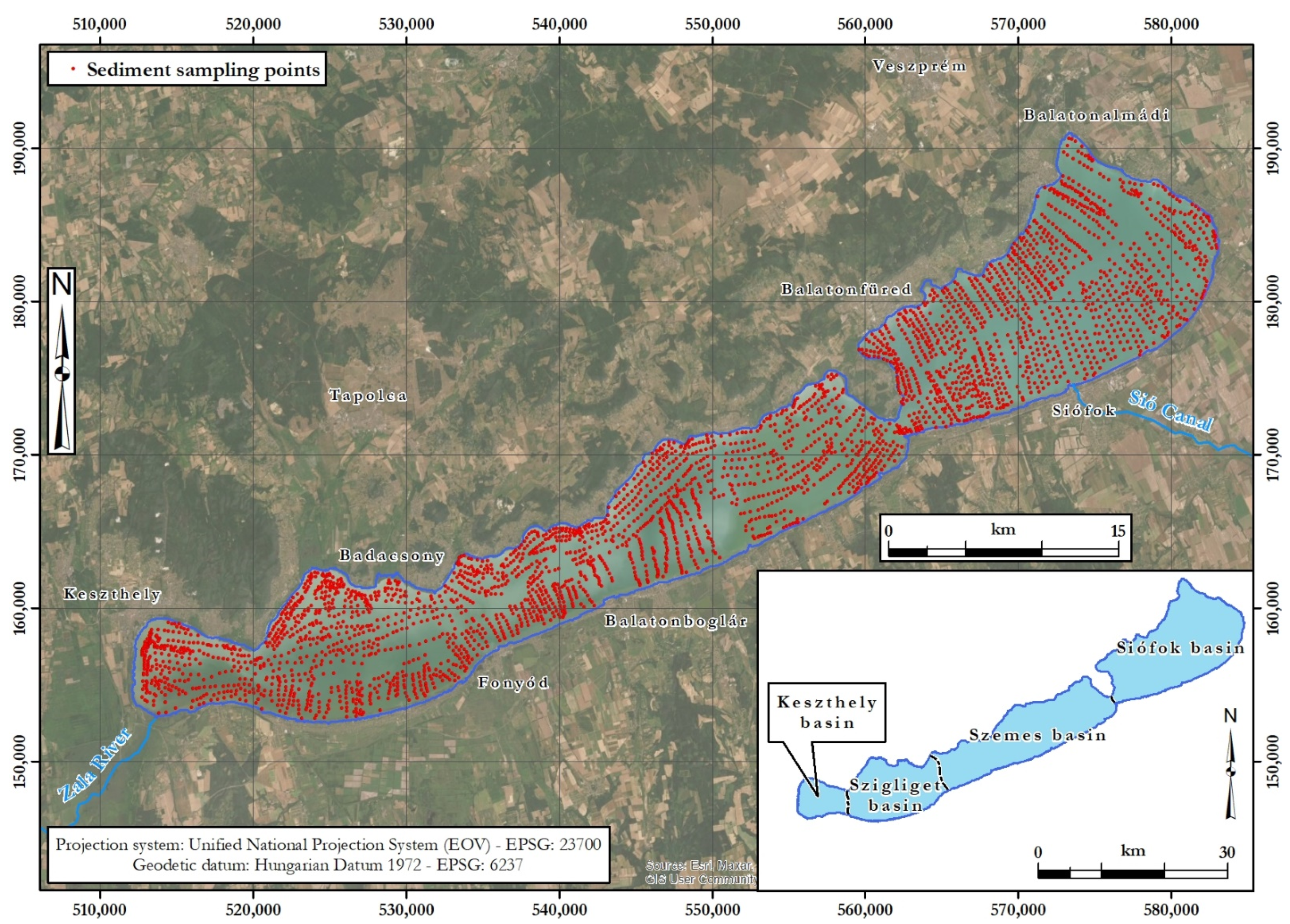
2.1. Sediment Sampling and Acquired Data on Nutrients

Between 1978 and 1984, a detailed survey was conducted on Lake Balaton, which was aimed at examining the physicochemical properties of the lake sediments, including N and P content, and then evaluating the environmental status of the lake [40,41]. Sediment samples were taken from the uppermost 10 cm of the sediment layer. In total, 3340 samples were collected (Figure 1) and then taken for laboratory analysis where P (to be more precise phosphorus pentoxide, i.e., P₂O₅) content (unit: mg kg⁻¹) extracted with ammonium lactate was determined photometrically, whilst total N content (unit: mg kg⁻¹) was measured by the method of Kjeldahl [42] according to the Hungarian soil and sediment analysis methodology standards in force at that time. Since the data on P were expressed in P₂O₅, first, we had to convert them to P content. This can be readily achieved by multiplying the data expressed in P₂O₅ by 0.437, which follows from stoichiometry. Hereafter, the data on P content (unit: mg kg⁻¹) and on N content (unit: mg kg⁻¹) were used.

We randomly split the data set on nutrients into a training set and a control set, where 80% of the data went to the training data set on which exploratory data analysis and multivariate geostatistical modeling were conducted. The remaining 20% of the nutrients data went to the control data set, which was independent throughout this study and only used for validation.

2.2. Variography

Most geostatistical techniques are only optimal if the variable under study is normally distributed [43]. We therefore transformed the data on N and P to normal scale by using normal score transformation, which is a type of quantile transformation based on Gaussian anamorphosis [23,44], and then spatial analysis and modeling were conducted on the transformed, normal scale.

We performed variography on the transformed N and P data in order to explore, analyze, and model (i) the spatial continuity of each nutrient separately and (ii) the spatial interdependence between the nutrients. The spatial continuity (or variability) of a nutrient was measured by (direct)variogram, which shows the average dissimilarity between data on the given nutrient separated by a vector [23]. It is commonly estimated by Matheron’s [45] method-of-moments estimator that is

$$\gamma \left(h\right)=\frac{1}{2n\left(h\right)}{\displaystyle \sum }_{i=1}^{n\left(h\right)}{\left[z\left(u_i\right)-z\left(u_i+h\right)\right]}^2$$

(1)

where $\gamma \left(h\right)$ is the variogram, $h$ is the separation vector, $n\left(h\right)$ is the number of data pairs separated by the vector $h$, and $z\left(u_i\right)$ and $z\left(u_i+h\right)$ are the observed value of the given nutrient at location $u_i$ and $u_i+h$, respectively. The joint spatial variability (or spatial cross-continuity) of N and P was measured by the cross-variogram, which shows how the two nutrients jointly vary in space [23]. Its method-of-moments estimator is

$${\gamma }_{\mathrm{NP}}\left(h\right)=\frac{1}{2n\left(h\right)}{\displaystyle \sum }_{i=1}^{n\left(h\right)}\left[z_{\mathrm{N}}\left(u_i\right)-z_{\mathrm{N}}\left(u_i+h\right)\right]·\left[z_{\mathrm{P}}\left(u_i\right)-z_{\mathrm{P}}\left(u_i+h\right)\right]$$

(2)

where ${\gamma }_{\mathrm{NP}}\left(h\right)$ is the cross-variogram between the nutrients N and P, and $z_{\mathrm{N}}\left(u_i\right)$ and $z_{\mathrm{P}}\left(u_i\right)$ are the observed values of N and P at location $u_i$, respectively. We should note that Equation (2) implies that both nutrients are measured at each sampling location, a situation referred to as isotopic case [23,24,25].

After computing the direct and cross-variograms of the transformed N and P data, a linear model of coregionalization was fitted, which ensures that a statistically valid model is used in further spatial modeling [23].

2.3. Multivariate Geostatistical Modeling

Based on the fitted linear model of coregionalization, a multivariate geostatistical model was built to model the joint spatial variability of the nutrients N and P. We used sequential stochastic cosimulation instead of cokriging due to two reasons. First, there is no analytical geostatistical solution to predict a spatial average or total over a region in case a nonlinear transformation (e.g., normal score transformation) is applied prior to geostatistical modeling [39]. Second, analytical derivation of the ratio of correlated random variables could be problematic and often needs stringent assumptions made on the distribution of the random variables. Thus, cosimulation was used to generate possible realities, i.e., stochastic realizations, of the multivariate geostatistical model built to the nutrients N and P. For both nutrients, 1000 stochastic realizations were generated with a spatial resolution of 100 m. The generated realizations were conditional to the N and P data and reproduced their joint spatial variability. Latter advantageous property of the realizations enables deriving stochastic realizations for the N:P ratio too. Therefore, we transformed the stochastic realizations of N and P back to the original scale, and then the stochastic realizations of the N:P ratio were derived by dividing the paired back-transformed realizations of N and P.

We provided point-support predictions with the same spatial resolution as used to generate the stochastic realizations (i.e., 100 m). Point-support prediction for the nutrients N and P and for the N:P ratio at a given point was identified by the mean of the 1000 stochastic realizations generated for the nutrients N and P and for the N:P ratio at that point, respectively.

2.4. Spatial Aggregation

In spatial aggregation, we used the back-transformed realizations to predict the spatial average of the nutrients N and P and the N:P ratio for the basins of Lake Balaton (Figure 1, inset map) and for the entire lake. The spatial average of a given nutrient or the N:P ratio over a given basin was obtained by first averaging the simulated values falling in that basin for each realization. This yielded 1000 average values for that basin, which could be interpreted as 1000 realizations of the basin average. Second, we took the average of the 1000 basin averages to obtain a prediction for the spatial average over that basin. This was performed for predicting the spatial average of N, P, and the N:P ratio for all basins. The same was carried out when predicting the spatial average of N, P, and the N:P ratio over the entire lake targeted, i.e., averaging the stochastic realizations to generate lake averages and then taking their average to provide a prediction for the spatial average over the entire lake.

2.5. Quantification of Uncertainty

Nowadays, end-users are interested not just in spatial prediction but in the associated prediction uncertainty as well [30]. We therefore computed the 90% prediction interval (PI), which is an interval within which the true value is expected to occur 9 times out of 10. We used the stochastic realizations for quantifying the prediction uncertainty not just for the nutrients N and P but also for the N:P ratio. At point support, the 90% PIs for N, P, and the N:P ratio were determined by the 0.05 and 0.95 quantiles of the 1000 simulated values of N, P, and the N:P ratio, respectively. In spatial aggregation, the 90% PIs for the spatial averages were determined by the 0.05 and 0.95 quantiles of the basin or lake averages.

2.6. Validation

The control data set was used to evaluate the performance of spatial predictions and uncertainty quantifications for N, P, and the N:P ratio at point support. We computed the most common error measures, i.e., mean error (ME) (also known as bias) and root mean square error (RMSE) (also known as the spread of the error distribution):

$$ME=\frac{1}{m}{\displaystyle \sum }_{i=1}^m\left[P\left(u_i\right)-O\left(u_i\right)\right]$$

(3)

$$RMSE=\sqrt{\frac{1}{m}{\displaystyle \sum }_{i=1}^m{\left[P\left(u_i\right)-O\left(u_i\right)\right]}^2}$$

(4)

where $m$ is the number of observations in the control data set, and $P\left(u_i\right)$ and $O\left(u_i\right)$ are the predicted and observed values at control location $u_i$, respectively. In addition to these measures, we also computed Lin’s [46] concordance correlation coefficient (CCC) and the Nash–Sutcliffe [47] model efficiency coefficient (NSE):

$$CCC=\frac{2{{\displaystyle \sum }}_{i=1}^m\left[O\left(u_i\right)-\overline{O}\right]·\left[P\left(u_i\right)-\overline{P}\right]}{{{\displaystyle \sum }}_{i=1}^m{\left[O\left(u_i\right)-\overline{O}\right]}^2+{{\displaystyle \sum }}_{i=1}^m{\left[P\left(u_i\right)-\overline{P}\right]}^2+{\left[\overline{O}-\overline{P}\right]}^2}$$

(5)

$$NSE=1-\frac{{{\displaystyle \sum }}_{i=1}^m{\left[P\left(u_i\right)-O\left(u_i\right)\right]}^2}{{{\displaystyle \sum }}_{i=1}^m{\left[O\left(u_i\right)-\overline{O}\right]}^2}$$

(6)

where $\overline{P}$ and $\overline{O}$ are the mean of the predicted and observed values, respectively.

Accuracy plots (also known as prediction interval coverage probability plot) and G statistics were used to evaluate uncertainty quantifications [30]. An accuracy plot graphically presents the observed fraction of control data falling within symmetric PIs of varying width. If uncertainty quantification is a realistic assessment of uncertainty, then the observed and expected fraction should take values close to each other. For instance, in such cases, about 90% of the validation data would fall within the 90% PI. If the observed fraction is higher than the expected fraction, then the uncertainty has been overestimated. If it is lower, the uncertainty has been underestimated. Ideally, the observed fractions follow the $x=y$ line on an accuracy plot. The G statistics measure the overall closeness of the accuracy plot to that line by

$$G=1-\underset{0}{\overset{1}{{\displaystyle \int }}}\left|\xi \left(p\right)-p\right|dp$$

(7)

where $\xi \left(p\right)$ and $p$ are the observed and expected fraction for a $p$-width symmetric PI, respectively. Ideally, G is equal to 1.

3. Results

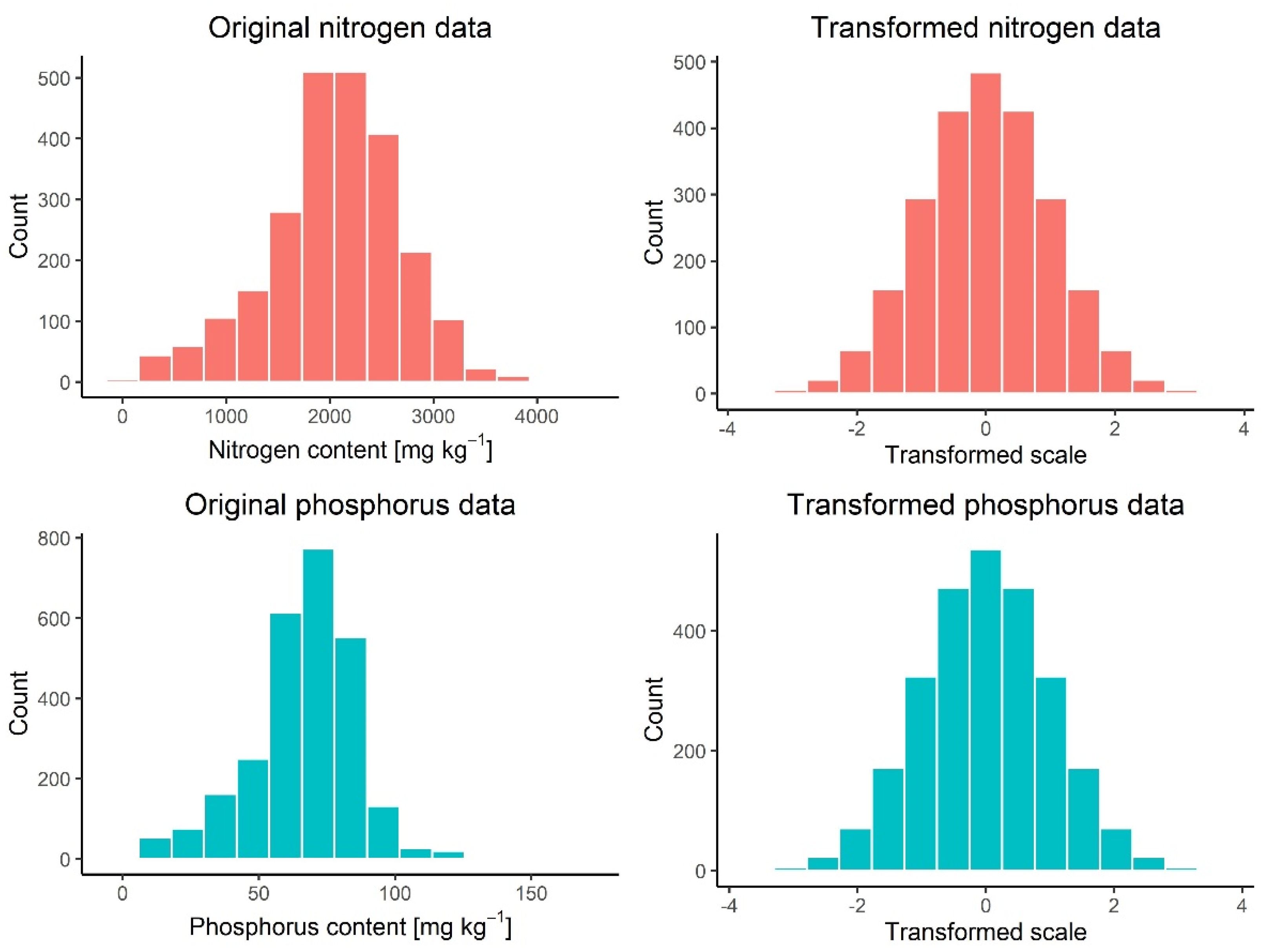
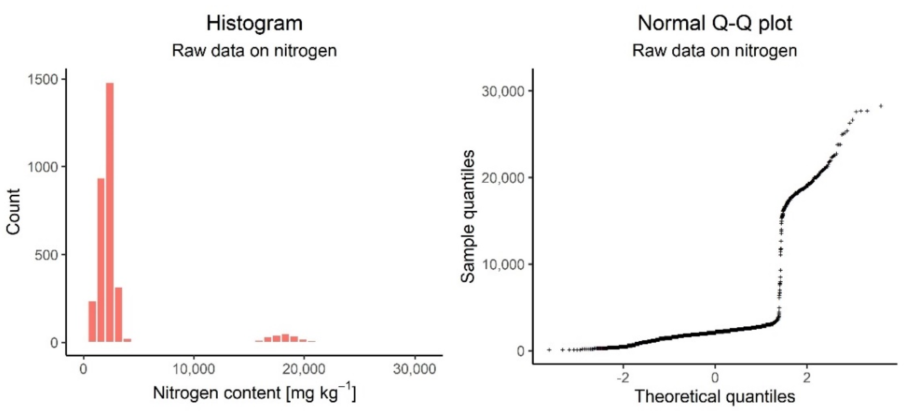
3.1. Exploratory Data Analysis

Exploratory data analysis on nutrients data showed that in the case of N content, there are about 250 observations that take extremely high values and seem to constitute another statistical ‘population’. These observations could be easily identified by the histogram in which they show an extra mode around 18,000 mg kg⁻¹ (Figure 2, left graph), which is also confirmed by the compiled Q-Q plot (Figure 2, right graph). All the observations with extremely high N content were collected in the Keszthely basin (Figure 1, inset map). We should note that in the case of nutrient P, there were no such extreme (or even outlier) values in that basin. In fact, extreme algae bloom occurred when the sampling campaign was conducted on the Keszthely basin (i.e., summer in 1978), and therefore, the basin was hypertrophic, which could cause such an extreme N content in the sediments [1,9,40]. Although these N observations could be realistic, we found that it is better to exclude them from the further geostatistical analysis, as they represent an extreme event (i.e., hypertrophic status) in the Keszthely basin and therefore could lead to bias, especially when geostatistical modeling of the entire lake is targeted.

Table 1. Summary statistics of nitrogen and phosphorus content measured in the sediments of Lake Balaton. Abbreviations: n: number of observations, SD: standard deviation.

Nutrient	Unit	n	Min	Max	Mean	Median	SD
Nitrogen	mg kg−1	2426	100	4500	2040	2100	634.63
Phosphorus	mg kg−1	2672	3.49	170.86	66.61	68.17	19.27

summarizes descriptive statistics of the nutrients N and P measured in the sediments of Lake Balaton after excluding N observations with extremely high values.

3.2. Variography and Multivariate Geostatistical Modeling

Figure 3 shows the histograms of the original (i.e., untransformed) and normal score transformed data on both nutrients. We should note that the transformed data have a standard normal distribution for both nutrients with zero mean and unit variance.

Figure 4 (open circles) presents the computed direct and cross-variograms for the nutrients N and P. The cross-variogram confirmed our preliminary hypothesis, i.e., there is a spatial interdependence between the two nutrients (Figure 4, right graph). This also means that it is better to jointly model their spatial distribution using multivariate geostatistics. We should note that cross-variogram (Equation (2)) can be computed only if data on both nutrients are available at the same location, i.e., the case is isotopic (see Section 2.2). However, this is not the case anymore since we had to exclude almost all the N content observations located in the Keszthely basin due to their extremely high values. Therefore, we had to constrain the computation of the cross-variogram between N and P for those sampling points at which data on both nutrients are available. Furthermore, we should assume that the spatial variability of N and the joint spatial variability between N and P observed in the rest of the lake is also applicable to the Keszthely basin. Nonetheless, we should note that data on P are still available for the Keszthely basin, which can help to model the spatial variability of N in that basin by exploiting the spatial cross-correlation (Figure 4, right graph) between the two nutrients.

We observed that the spatial variability of both nutrients showed nested structure, which could be also identified on the computed cross-variogram. Therefore, the fitted linear model of coregionalization (Figure 4, solid lines) has also a nested structure to describe the spatial variability of the nutrients under study realistically. The first structure models discontinuity at the origin (i.e., nugget effect). This can be attributed to (i) short-scale variability that is shorter than the minimum distance between the sampling points and/or (ii) to measurement error [23]. The second and third structures model a short and a larger scale of spatial continuity with a range value of 3.5 km and 20 km, respectively.

Table 2. Shapes and parameters of the linear model of coregionalization fitted to the experimental direct and cross-variograms presented in Figure 4.

	Model Type	Partial Sill	Range [km]
Variogram Nitrogen	Nugget	0.2726	0
	Spherical	0.4199	3.5
	Spherical	0.3845	20
Variogram Phosphorus	Nugget	0.0723	0
	Spherical	0.2835	3.5
	Spherical	0.7612	20
Cross-variogram Nitrogen and Phosphorus	Nugget	0.0063	0
	Spherical	0.0320	3.5
	Spherical	0.3413	20

gives a summary of the shapes and parameters of the fitted linear model of coregionalization presented in Figure 4 (solid lines).

Based on the fitted linear model of coregionalization, a multivariate geostatistical model was built to model the joint spatial variability of the nutrients N and P. In total, 1000 stochastic realizations were generated for each nutrient by using stochastic cosimulation, and then 1000 realizations for the N:P ratio were derived by dividing the paired back-transformed realizations of N and P.

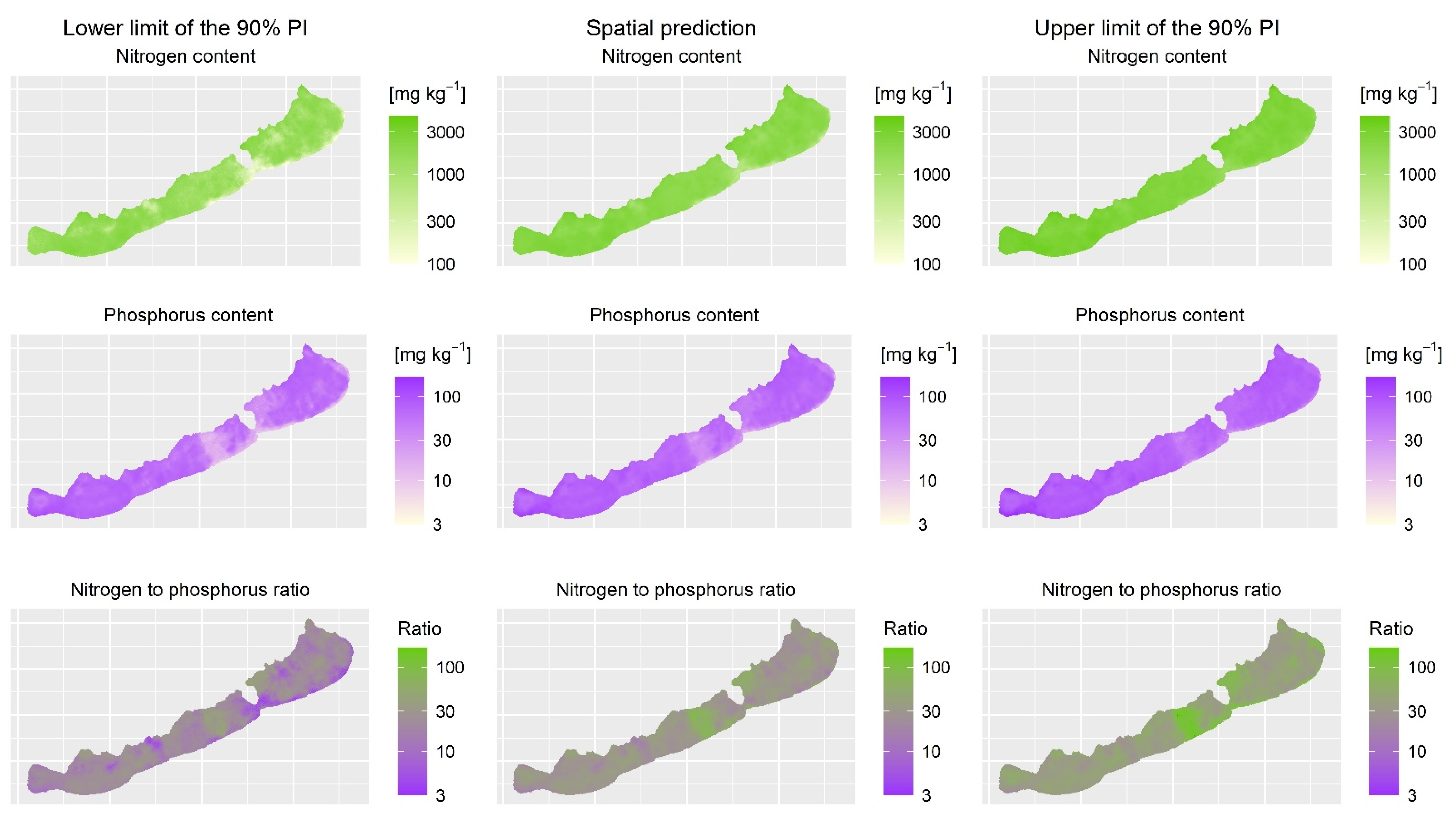
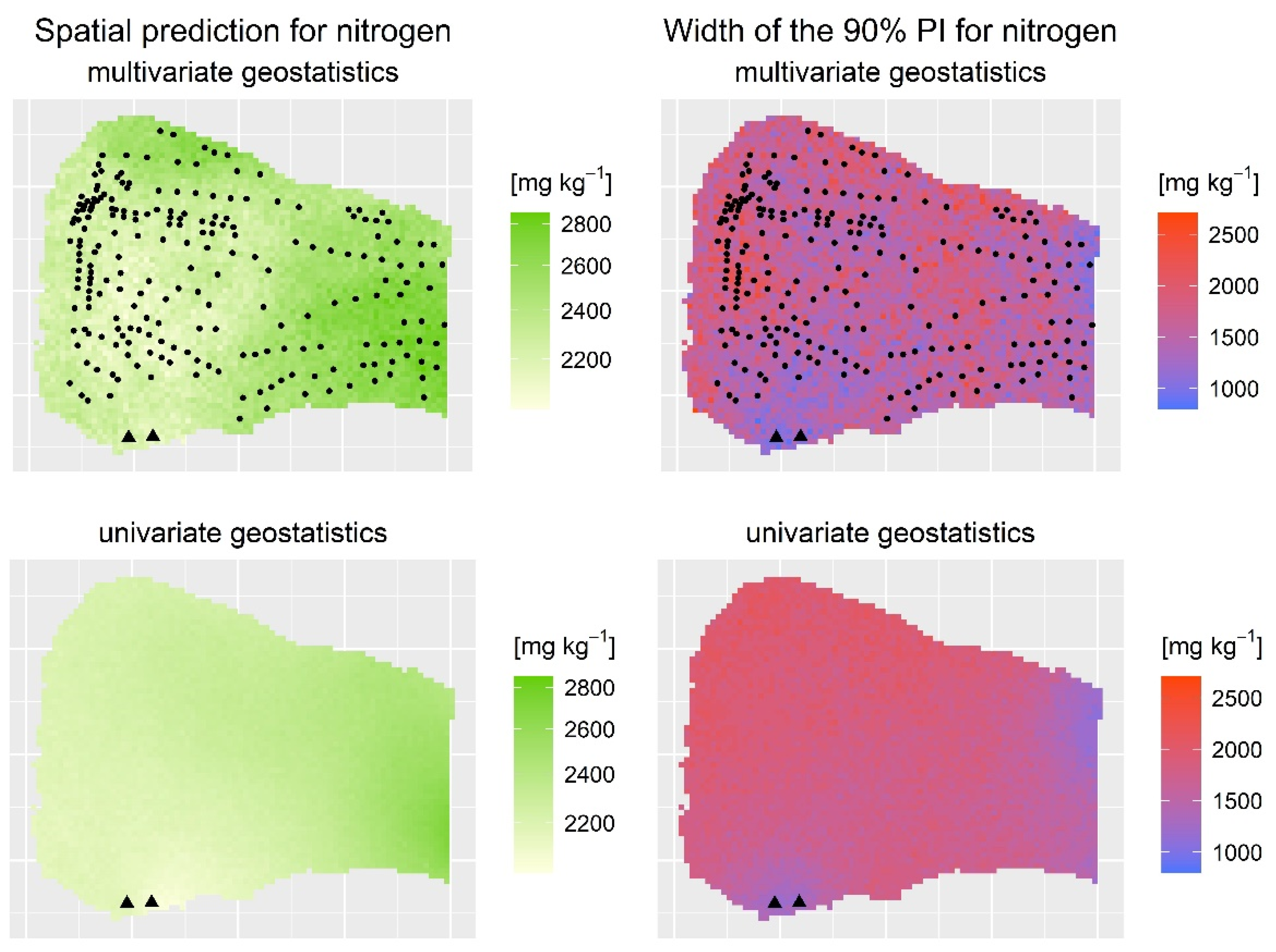
3.3. Spatial Prediction at Point Support

Based on the stochastic realizations generated by sequential stochastic cosimulation, we predicted the spatial distribution of the nutrients N and P and the N:P ratio at point support with a resolution of 100 m. Figure 5 (middle column) presents the point-support predictions for the sediments of Lake Balaton. Note that predictions refer to the uppermost 10 cm of the sediment layer of the lake. In addition to the spatial predictions, we also quantified the associated prediction uncertainty, which was expressed by the upper and lower limit of the 90% PI that is frequently used in environmental mapping (e.g., [27,29,48]), as presented in Figure 5 (left and right columns).

Figure 6 gives a more detailed picture of the Keszthely basin where most of the N observations had to be excluded from spatial modeling and only data on P were available. Based on Figure 6, it is apparent that taking the P data into account and exploiting the spatial cross-correlation existing between the nutrients (Figure 4, right graph) in the course of spatial modeling (Figure 6, first row) can lead to a more appropriate prediction compared to the case when using univariate geostatistics based only on the variogram of N (Figure 4, left graph) and thus ignoring spatial cross-correlation completely (Figure 6, last row). Furthermore, the associated prediction uncertainty modeled and quantified by multivariate geostatistics is smaller than that quantified by univariate geostatistics (Figure 6, last column). Note that in Figure 6 we expressed prediction uncertainty by the width of the 90% PI, which can be interpreted as the wider the PI, the larger the prediction uncertainty.

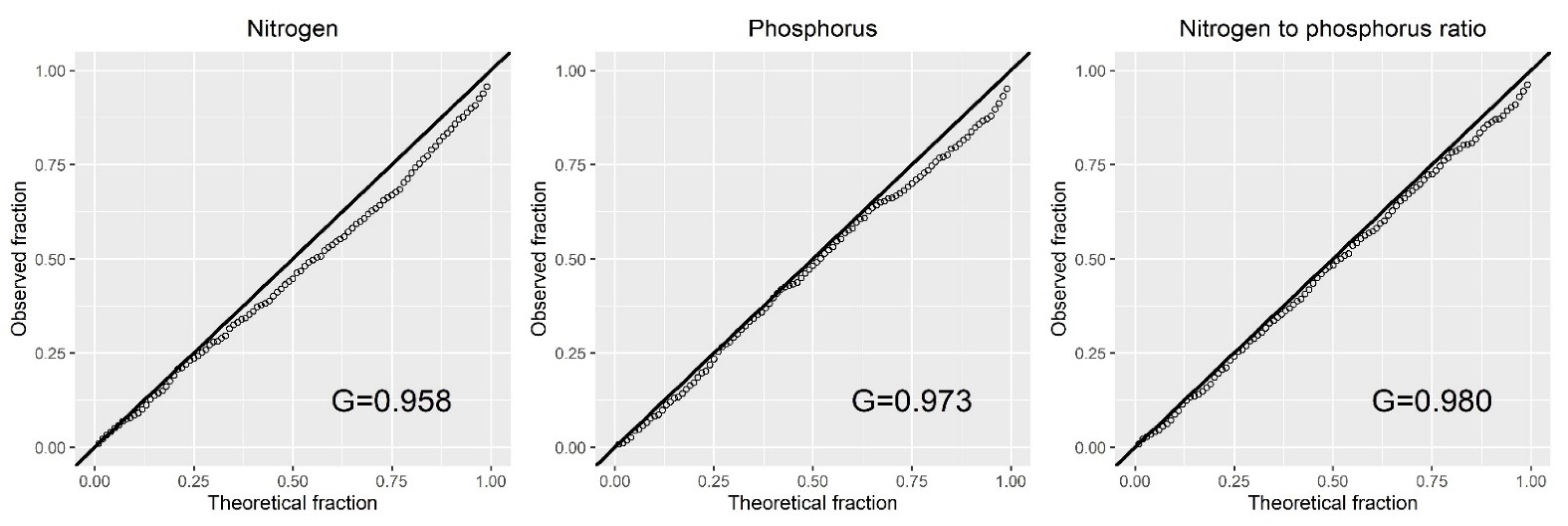
3.4. Performance of Spatial Predictions and Uncertainty Quantifications

Table 3. Validation of nitrogen, phosphorus, and nitrogen-to-phosphorus ratio spatial predictions at point support. Abbreviations: ME: mean error, RMSE: root mean square error, CCC: Lin’s concordance correlation coefficient, NSE: Nash–Sutcliffe model efficiency coefficient, N:P ratio: nitrogen-to-phosphorus ratio.

	ME	RMSE	CCC	NSE
Nitrogen	7.61	463.93	0.65	0.48
Phosphorus	0.34	8.56	0.89	0.80
N:P ratio	0.09	12.54	0.52	0.31

gives a summary of the validation measures introduced in Section 2.6, which were used to evaluate the performance of the spatial predictions at point support. An important aim of every spatial modeling procedure is to provide unbiased spatial predictions (i.e., value of ME close to zero) with RMSE as low as possible. The values of ME range from 0.09 to 7.61 with relatively low RMSE values (i.e., 8.56, 12.54, and 463.93 for P, N:P, and N, respectively), which means that the multivariate geostatistical model gave fairly unbiased spatial predictions for both nutrients and for the N:P ratio too. Additionally, the values of CCC range from 0.52 to 0.89, which also confirms that the accuracy of the spatial predictions is acceptable. NSE can be interpreted as the value of R-square if its value is greater than zero. The values of NSE range from 0.31 to 0.80.

We checked the performance of the uncertainty quantifications at point support by accuracy plots and G statistics. Figure 7 shows the accuracy plots (Figure 7, open circles) and computed G statistics for both sediment nutrients and for the N:P ratio. The accuracy plots quasi follow the $x=y$ line (Figure 7, solid lines), which proves that the accuracy of uncertainty quantifications is acceptable. This observation is also confirmed by the computed G statistics, which are close to the expected value (i.e., 1).

3.5. Spatial Aggregation

Table 4. Spatial averages for the basins and for the entire lake as results of spatial aggregation. Annotation: numbers in square brackets present the upper and lower limit of the 90% prediction interval as a measure of spatial uncertainty. Abbreviation: N:P ratio: nitrogen-to-phosphorus ratio.

	Spatial Average	Spatial Average	Spatial Average
	Nitrogen	Phosphorus	N:P Ratio
Keszthely basin	2383.15 mg kg−1	87.56 mg kg−1	28.76
	[2005.15; 2775.96]	[86.29; 88.87]	[23.77; 33.91]
Szigliget basin	2389.21 mg kg−1	78.74 mg kg−1	30.68
	[2361.82; 2416.21]	[78.26; 79.20]	[30.30; 31.07]
Szemes basin	1920.13 mg kg−1	59.39 mg kg−1	36.63
	[1893.33; 1947.10]	[58.84; 59.96]	[35.71; 37.57]
Siófok basin	1950.68 mg kg−1	63.31 mg kg−1	32.39
	[1927.07; 1971.57]	[62.88; 63.74]	[31.88; 32.86]
Lake Balaton	2063.51 mg kg−1	66.94 mg kg−1	33.17
	[2035.44; 2092.69]	[66.68; 67.22]	[32.67; 33.70]

summarizes the results of spatial aggregation and presents not just the predicted spatial average of the nutrients N and P and the N:P ratio for the four basins of Lake Balaton and for the entire lake but also the associated prediction uncertainty (Table 4, numbers in square brackets). In the sediments of the western one-third of the lake (i.e., Keszthely and Szigliget basins (see Figure 1, inset map)), the N and P content is higher than in the sediments of the eastern two-third (i.e., Szemes and Siófok basins). Additionally, based on the predicted spatial averages of the N:P ratio, it can be highlighted that not just the absolute P content but also its relative content to the N content is higher in the western part of the lake where most algae blooms occur. These findings are in line with the results reported by previous studies conducted on the lake (e.g., [9,49,50,51]). If we compare the uncertainty of point-support predictions (Figure 5) with the uncertainty of spatial averages (Table 4, numbers in square brackets), it can be seen that the uncertainty associated with the spatial average is smaller. This can be attributed to the fact that negative and positive interpolation errors partially cancel out when values are aggregated, a phenomenon well-known in geostatistics [26,39,52]. We should also highlight that in the Keszthely basin the prediction uncertainty of spatial averages is the highest for the N content and for the N:P ratio. This can be explained by the fact that most of the N observations had to be excluded from geostatistical modeling and only data on P were available in that basin. Nonetheless, we should note that the prediction uncertainty would have been much higher if we had not used the P data available for that basin (see Figure 6, last column). Thus, P data available for the basin came in handy when spatial modeling of N content was targeted thanks to the cross-correlation existing between the two nutrients.

4. Discussion

Although there are a number of textbooks (e.g., [23,24,25,26,44,53]) introducing the theory and application of multivariate geostatistics in earth and environmental sciences, it is rarely used in practice. Most of the studies in which spatial modeling of more than one variable is targeted still apply univariate geostatistics without taking into account the probable existing spatial interdependence between the variables under study and then model their spatial variability separately. This practice may lead to incoherent results and therefore to inappropriate conclusions, especially when a complex assessment is planned to be carried out on these spatial models. Indeed, some studies pointed out that separately kriged composite data, whose sum should be a fixed number (e.g., the particle size fractions (i.e., sand, silt, and clay content) of soils sum to 100%) or whose difference cannot be negative (e.g., depth of shallow groundwater level computed as surface elevation minus the elevation of shallow groundwater level), will yield incoherent results, as their sum will not be 100% or their difference will be negative at some locations of the area under study (e.g., [18,54,55,56]). However, multivariate geostatistics indeed is able to provide such coherent results, which are highly appreciated in further assessments.

As it has been illustrated in the example of Lake Balaton, multivariate geostatistics is able to explicitly take the spatial interdependence existing between the variables under study into account. Additionally, we should also highlight that it simultaneously exploits this interdependence, especially when one variable is undersampled to the other(s), as we have seen in the example of N content (Figure 6). Due to the extremely high values, we had to exclude most of the N observations in the Keszthely basin, and only data on P content were available in the basin. Nonetheless, in spatial modeling of N content, we could take these P data into account by using the spatial cross-correlation between the two nutrients (Figure 4, right graph), which is a well-known, advantageous property of multivariate geostatistics [23,24,26]. A number of papers have pointed out that by using a multivariate geostatistical approach, a more accurate spatial model can be gained for an undersampled variable if one (or even more) densely sampled variable is also available [54,57,58,59].

The proposed methodology also has the advantage of generating such stochastic realizations, which reproduce the joint spatial variability of the variables under study. Indeed, this allowed the derivation of the stochastic realizations of the two nutrients’ ratios, which were then used for providing spatial prediction for the N:P ratio with the associated prediction uncertainty. Although it is also an attractive feature of multivariate geostatistics, it is still rarely exploited in practice. In addition, Szatmári et al. [39] pointed out that an approach that does not account for the spatial cross-correlation between the variables under study will fail to characterize the uncertainty about the derived variable reliably.

As it has been pointed out in the Introduction (Section 1), the end-users often need spatially explicit information on water quality indicators at a larger support than that on which sampling and laboratory measurement have been conducted [17,32,33,34,35], a situation referred to as change-of-support in geostatistics. It calls for upscaling to make spatial predictions and the associated uncertainty appropriate for the end-users’ requirements. In this study, we proposed an approach based on spatial aggregation of the generated stochastic realizations that can be used not just to predict the spatial average for a given area or region but also to quantify the uncertainty associated with the prediction. Although nutrients and their ratio were spatially aggregated only at the support of basins and the entire lake, the generated stochastic realizations allow carrying out spatial aggregation at various supports, whatever their shape and size.

5. Conclusions

The objective of our study was to illustrate the merits of applying multivariate geostatistics when spatial modeling of more than one variable is targeted at various scales in water ecosystems. These merits were illustrated in the example of Lake Balaton’s sediments, where a methodology based on multivariate geostatistics was elaborated and used to jointly model the spatial distribution of the nutrients N and P and their ratio (i.e., N:P) and then provide spatial predictions at different scales with the associated prediction uncertainty. Our study highlighted that it is worthy of applying multivariate geostatistics in case spatial modeling of two or more variables, which show spatial interdependence, is targeted in water ecosystems. By the application of multivariate geostatistics, the spatial interdependence existing between the variables under study can be explicitly taken into account and exploited in the course of spatial modeling to provide coherent and more accurate spatial models that support the complex assessment of the water quality and environmental status of lakes. Additionally, the generated stochastic realizations, reproducing the joint spatial variability of the variables under study, allow deriving further variables based on those involved into the stochastic cosimulation. Furthermore, to provide spatially aggregated predictions for larger supports (e.g., basins or entire lake) with the associated prediction uncertainty, which may better fit the end-users’ demands on spatially explicit information about water ecosystems.

References

1. Herodek, S. The eutrophication of Lake Balaton: Measurements, modeling and management. In SIL Proceedings, 1922–2010; Taylor and Francis: Abingdon, UK, 1984; Volume 22, pp. 1087–1091. [Google Scholar] [CrossRef]
2. Hatvani, I.G.; Clement, A.; Kovács, J.; Kovács, I.S.; Korponai, J. Assessing water-quality data: The relationship between the water quality amelioration of Lake Balaton and the construction of its mitigation wetland. J. Great Lakes Res. 2014, 40, 115–125. [Google Scholar] [CrossRef]
3. Istvánovics, V.; Clement, A.; Somlyódy, L.; Specziár, A.; László, G.; Padisák, J. Updating water quality targets for shallow Lake Balaton (Hungary), recovering from eutrophication. Hydrobiologia 2007, 581, 305–318. [Google Scholar] [CrossRef]
4. Bostrom, B.; Pettersson, K. Different patterns of phosphorus release from lake sediments in laboratory experiments. Hydrobiologia 1982, 91, 415–429. [Google Scholar] [CrossRef]
5. Hutchinson, G.E. A Treatise on Limnology I.: Geography, Physics and Chemistry; Wiley: New York, NY, USA, 1957. [Google Scholar]
6. Wetzel, R.G. Limnology; Saunders: Philadelphia, PA, USA, 1975. [Google Scholar]
7. Williams, J.D.H.; Syers, J.K.; Harris, R.F.; Armstrong, D.E. Fractionation of Inorganic Phosphate in Calcareous Lake Sediments. Soil Sci. Soc. Am. J. 1971, 35, 250–255. [Google Scholar] [CrossRef]
8. Istvanovics, V.; Somlyody, L. Factors influencing lake recovery from eutrophication—The case of Basin 1 of Lake Balaton. Water Res. 2001, 35, 729–735. [Google Scholar] [CrossRef]
9. Hatvani, I.G.; de Barros, V.D.; Tanos, P.; Kovács, J.; Székely Kovács, I.; Clement, A. Spatiotemporal changes and drivers of trophic status over three decades in the largest shallow lake in Central Europe, Lake Balaton. Ecol. Eng. 2020, 151, 105861. [Google Scholar] [CrossRef]
10. Istvánovics, V. Seasonal variation of phosphorus release from the sediments of Shallow Lake Balaton (Hungary). Water Res. 1988, 22, 1473–1481. [Google Scholar] [CrossRef]
11. Istvánovics, V.; Herodek, S.; Szilágyi, F. Phosphate adsorption by different sediment fractions in Lake Balaton and its protecting reservoirs. Water Res. 1989, 23, 1357–1366. [Google Scholar] [CrossRef]
12. Marinović, Z.; Tokodi, N.; Backović, D.D.; Šćekić, I.; Kitanović, N.; Simić, S.B.; Đorđević, N.B.; Ferincz, Á.; Staszny, Á.; Dulić, T.; et al. Does the kis-balaton water protection system (Kbwps) effectively safeguard lake balaton from toxic cyanobacterial blooms? Microorganisms 2021, 9, 960. [Google Scholar] [CrossRef]
13. Kocsis, M.; Szatmári, G.; Kassai, P.; Kovács, G.; Tóth, J.; Krámer, T.; Torma, P.; Homoródi, K.; Pomogyi, P.; Szeglet, P.; et al. Soluble phosphorus content of Lake Balaton sediments. J. Maps 2022. [Google Scholar] [CrossRef]
14. Downing, J.A.; McCauley, E. The nitrogen: Phosphorus relationship in lakes. Limnol. Oceanogr. 1992, 37, 936–945. [Google Scholar] [CrossRef] [Green Version]
15. Présing, M.; Preston, T.; Takátsy, A.; Sprőber, P.; Kovács, A.W.; Vörös, L.; Kenesi, G.; Kóbor, I. Phytoplankton nitrogen demand and the significance of internal and external nitrogen sources in a large shallow lake (Lake Balaton, Hungary). Hydrobiologia 2008, 599, 87–95. [Google Scholar] [CrossRef]
16. Vörös, L.; Göde, P.N. Long term changes of phytoplankton in Lake Balaton (Hungary). Int. Ver. Für Theor. Und Angew.Limnol. Verh. 1993, 25, 682–686. [Google Scholar] [CrossRef]
17. Kovács, J.; Nagy, M.; Czauner, B.; Kovács, I.S.; Borsodi, A.K.; Hatvani, I.G. Delimiting sub-areas in water bodies using multivariate data analysis on the example of Lake Balaton (W Hungary). J. Environ. Manag. 2012, 110, 151–158. [Google Scholar] [CrossRef]
18. Magyar, N.; Hatvani, I.G.; Székely, I.K.; Herzig, A.; Dinka, M.; Kovács, J. Application of multivariate statistical methods in determining spatial changes in water quality in the Austrian part of Neusiedler See. Ecol. Eng. 2013, 55, 82–92. [Google Scholar] [CrossRef]
19. Blix, K.; Pálffy, K.; Tóth, V.R.; Eltoft, T. Remote sensing of water quality parameters over Lake Balaton by using Sentinel-3 OLCI. Water 2018, 10, 1428. [Google Scholar] [CrossRef] [Green Version]
20. Łopata, M.; Popielarczyk, D.; Templin, T.; Dunalska, J.; Wiśniewski, G.; Bigaj, I.; Szymański, D. Spatial variability of nutrients (N, P) in a deep, temperate lake with a low trophic level supported by global navigation satellite systems, geographic information system and geostatistics. Water Sci. Technol. 2014, 69, 1834–1845. [Google Scholar] [CrossRef] [PubMed]
21. Olsen, J.M.; Williams, G.P.; Miller, A.W.; Merritt, L.V. Measuring and calculating current atmospheric phosphorous and nitrogen loadings to Utah Lake using field samples and geostatistical analysis. Hydrology 2018, 5, 45. [Google Scholar] [CrossRef] [Green Version]
22. Sarah, S.; Jeelani, G.; Ahmed, S. Assessing variability of water quality in a groundwater-fed perennial lake of Kashmir Himalayas using linear geostatistics. J. Earth Syst. Sci. 2011, 120, 399–411. [Google Scholar] [CrossRef] [Green Version]
23. Goovaerts, P. Geostatistics for Natural Resources Evaluation; Oxford University Press: Oxford, UK, 1997; ISBN 9780195115383. [Google Scholar]
24. Wackernagel, H. Multivariate Geostatistics; Springer: Berlin/Heidelberg, Germany, 2003. [Google Scholar]
25. Cressie, N.A.C. Statistics for Spatial Data; Wiley: New York, NY, USA, 1993. [Google Scholar]
26. Webster, R.; Oliver, M.A. Geostatistics for Environmental Scientists, 2nd ed.; Wiley: New York, NY, USA, 2007; ISBN 0470028580. [Google Scholar]
27. Pásztor, L.; Szabó, K.Z.; Szatmári, G.; Laborczi, A.; Horváth, Á. Mapping geogenic radon potential by regression kriging. Sci. Total Environ. 2016, 544, 883–891. [Google Scholar] [CrossRef]
28. Tóth, G.; Hermann, T.; Szatmári, G.; Pásztor, L. Maps of heavy metals in the soils of the European Union and proposed priority areas for detailed assessment. Sci. Total Environ. 2016, 565, 1054–1062. [Google Scholar] [CrossRef]
29. Laborczi, A.; Bozán, C.; Körösparti, J.; Szatmári, G.; Kajári, B.; Túri, N.; Kerezsi, G.; Pásztor, L. Application of Hybrid Prediction Methods in Spatial Assessment of Inland Excess Water Hazard. ISPRS Int. J. Geo-Inf. 2020, 9, 268. [Google Scholar] [CrossRef]
30. Szatmári, G.; Pásztor, L. Comparison of various uncertainty modelling approaches based on geostatistics and machine learning algorithms. Geoderma 2019, 337, 1329–1340. [Google Scholar] [CrossRef]
31. Somlyódy, L.; van Straten, G. Modeling and Managing Shallow Lake Eutrophication with Application to Lake Balaton; Springer: Berlin/Heidelberg, Germany, 1986. [Google Scholar]
32. Tasnim, B.; Fang, X.; Hayworth, J.S.; Tian, D. Simulating nutrients and phytoplankton dynamics in lakes: Model development and applications. Water 2021, 13, 2088. [Google Scholar] [CrossRef]
33. Istvánovics, V.; Honti, M. Stochastic simulation of phytoplankton biomass using eighteen years of daily data—Predictability of phytoplankton growth in a large, shallow lake. Sci. Total Environ. 2021, 764, 143636. [Google Scholar] [CrossRef] [PubMed]
34. Chang, M.; Teurlincx, S.; Janse, J.H.; Paerl, H.W.; Mooij, W.M.; Janssen, A.B.G. Exploring how cyanobacterial traits affect nutrient loading thresholds in shallow lakes: A modelling approach. Water 2020, 12, 2467. [Google Scholar] [CrossRef]
35. Honti, M.; Gao, C.; Istvánovics, V.; Clement, A. Lessons Learnt from the Long-Term Management of a Large (Re)constructed Wetland, the Kis-Balaton Protection System (Hungary). Water 2020, 12, 659. [Google Scholar] [CrossRef] [Green Version]
36. Goovaerts, P. Sample Support. Encycl. Environ. 2012. [Google Scholar] [CrossRef]
37. Goovaerts, P. Geostatistical modelling of uncertainty in soil science. Geoderma 2001, 103, 3–26. [Google Scholar] [CrossRef]
38. Cressie, N. Block kriging for lognormal spatial processes. Math. Geol. 2006, 38, 413–443. [Google Scholar] [CrossRef]
39. Szatmári, G.; Pásztor, L.; Heuvelink, G.B.M. Estimating soil organic carbon stock change at multiple scales using machine learning and multivariate geostatistics. Geoderma 2021, 403, 115356. [Google Scholar] [CrossRef]
40. Csermák, K.; Máté, F. A Balaton Talaja; Veszprémi Egyetem Georgikon Kar: Keszthely, Hungary, 2004. [Google Scholar]
41. Máté, F. A Balaton-meder recens üledékeinek térképezése. Magy. Állami Földtani Intézet Évi Jelentése Az 1985. Évről 1987. [Google Scholar]
42. Kjeldahl, J. Neue Methode zur Bestimmung des Stickstoffs in organischen Körpern. Z. Für Anal. Chem. 1883, 22, 366–382. [Google Scholar] [CrossRef] [Green Version]
43. Geiger, J. Some thoughts on the pre- and post-processing in sequential gaussian simulation and their effects on reservoir characterization. In New Horizons in Central European Geomathematics, Geostatistics and Geoinformatics; Geiger, J., Pál-Molnár, E., Malvic, T., Eds.; GeoLitera: Szeged, Hungary, 2012; pp. 17–34. [Google Scholar]
44. Deutsch, C.V.; Journel, A.G. GSLIB: Geostatistical Software Library and User’s Guide; Oxford University Press: Oxford, UK, 1998; ISBN 9780195100150. [Google Scholar]
45. Matheron, G. Principles of geostatistics. Econ. Geol. 1963, 58, 1246–1266. [Google Scholar] [CrossRef]
46. Lin, L.I.-K. A Concordance Correlation Coefficient to Evaluate Reproducibility. Biometrics 1989, 45, 255. [Google Scholar] [CrossRef]
47. Nash, J.E.; Sutcliffe, J.V. River flow forecasting through conceptual models part I—A discussion of principles. J. Hydrol. 1970, 10, 282–290. [Google Scholar] [CrossRef]
48. Szatmári, G.; Bakacsi, Z.; Laborczi, A.; Petrik, O.; Pataki, R.; Tóth, T.; Pásztor, L. Elaborating Hungarian segment of the Global Map of Salt-affected Soils (GSSmap): National contribution to an international initiative. Remote Sens. 2020, 12, 4073. [Google Scholar] [CrossRef]
49. Herodek, S.; Istvánovics, V. Mobility of phosphorus fractions in the sediments of Lake Balaton. Hydrobiologia 1986, 135, 149–154. [Google Scholar] [CrossRef]
50. Buczkó, K.; Ács, É.; Báldi, K.; Pozderka, V.; Braun, M.; Kiss, K.T.; Korponai, J. The first high resolution diatom record from Lake Balaton, Hungary in Central Europe. Limnetica 2019, 38, 417–430. [Google Scholar] [CrossRef]
51. Sagehashi, M.; Sakoda, A.; Suzuki, M. A mathematical model of a shallow and Eutrophic Lake (The Keszthely Basin, Lake Balaton) and simulation of restorative manipulations. Water Res. 2001, 35, 1675–1686. [Google Scholar] [CrossRef]
52. Heuvelink, G.B.M. Error Propagation in Environmental Modelling with GIS; Taylor and Francis: Abingdon, UK, 1998; ISBN 074840743X. [Google Scholar]
53. Chilès, J.-P.; Delfiner, P. Geostatistics: Modeling Spatial Uncertainty, 2nd ed.; Wiley Blackwell: Hoboken, NJ, USA, 2012; ISBN 9780470183151. [Google Scholar]
54. Fehér, Z.Z.; Rakonczai, J. Analysing the sensitivity of Hungarian landscapes based on climate change induced shallow groundwater fluctuation. Hung. Geogr. Bull. 2019, 68, 355–372. [Google Scholar] [CrossRef]
55. Laborczi, A.; Szatmári, G.; Kaposi, A.D.; Pásztor, L. Comparison of soil texture maps synthetized from standard depth layers with directly compiled products. Geoderma 2019, 352, 360–372. [Google Scholar] [CrossRef]
56. Garamhegyi, T.; Hatvani, I.G.; Szalai, J.; Kovács, J. Delineation of Hydraulic Flow Regime Areas Based on the Statistical Analysis of Semicentennial Shallow Groundwater Table Time Series. Water 2020, 12, 828. [Google Scholar] [CrossRef] [Green Version]
57. McBratney, A.B.; Webster, R. Optimal interpolation and isarithmic mapping of soil properties. V. Co-regionalization and multiple sampling strategy. J. Soil Sci. 1983, 34, 137–162. [Google Scholar] [CrossRef]
58. Odeh, I.O.A.; McBratney, A.B.; Chittleborough, D.J. Spatial prediction of soil properties from landform attributes derived from a digital elevation model. Geoderma 1994, 63, 197–214. [Google Scholar] [CrossRef]
59. Odeh, I.O.A.; McBratney, A.B.; Chittleborough, D.J. Further results on prediction of soil properties from terrain attributes: Heterotopic cokriging and regression-kriging. Geoderma 1995, 67, 215–226. [Google Scholar] [CrossRef]
Figure 1. Location of sampling points (n = 3340) across Lake Balaton. The inset map (bottom right) shows the lake basins (from west to east): Keszthely, Szigliget, Szemes, and Siófok basin.
Water 14 00361 g001
Figure 2. Some graphical results of exploratory data analysis conducted on the raw nitrogen content data: histogram (left graph) and normal Q-Q plot (right graph).
Water 14 00361 g002
Figure 3. Histograms of the original (left column) and transformed (right column) data on the nutrients nitrogen and phosphorus. Annotation: the transformed data have a standard normal distribution for both nutrients with zero mean and unit variance.
Water 14 00361 g003
Figure 4. Experimental direct and cross-variograms (open circles) for the nutrients nitrogen and phosphorus and the fitted linear model of coregionalization (solid lines). Annotation: parameters of the fitted linear model of coregionalization can be found in Table 2.
Water 14 00361 g004
Figure 5. Point-support predictions for the nutrients nitrogen and phosphorus and for the nitrogen-to-phosphorus ratio (middle column) and the associated prediction uncertainty quantified by the upper (right column) and lower (left column) limit of the 90% prediction interval. Abbreviation: PI: prediction interval.
Water 14 00361 g005
Figure 6. Point-support predictions for the nutrient nitrogen (first column) and the associated prediction uncertainty (last column) in the Keszthely basin given by multivariate (first row) and univariate geostatistics (last row). Annotation: black dots represent sampling points where only phosphorus data are available, whereas black triangles mean sampling points where data on both nutrients are available. Abbreviation: PI: prediction interval.
Water 14 00361 g006
Figure 7. Accuracy plots (open circles) and computed G statistics for the nutrients nitrogen (left graph) and phosphorus (middle graph) and for nitrogen-to-phosphorus ratio (right graph). Abbreviation: G: G statistics.
Water 14 00361 g007