
SMODERP2D—Sheet and Rill Runoff Routine Validation at Three Scale Levels


Abstract
:1. Introduction
2. Materials and Methods
2.1. SMODERP2D
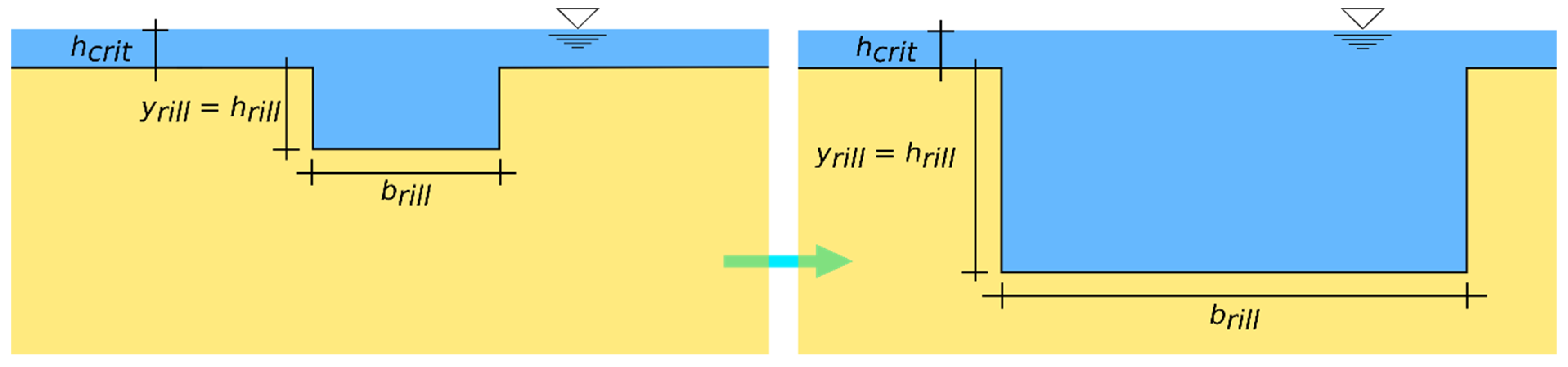
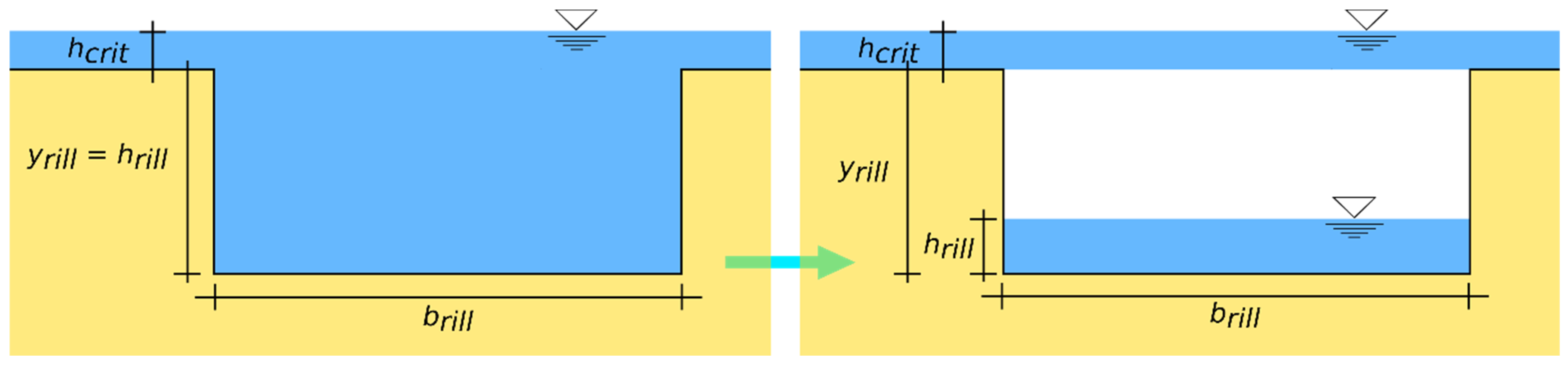
Rill Flow
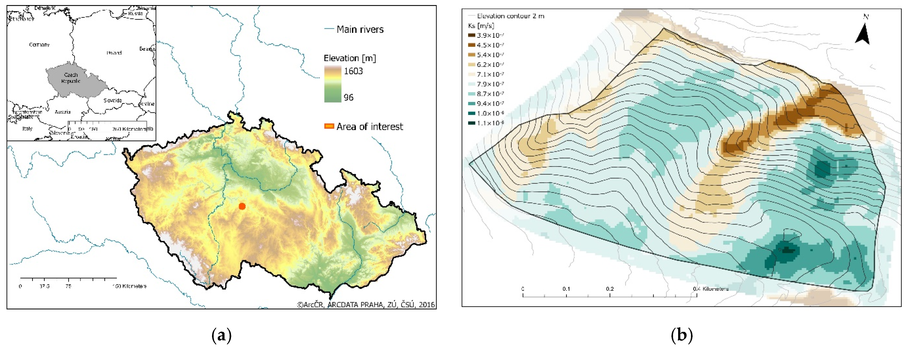
2.2. Study Site
2.3. Plot-Scale Sheet Flow Calibration and Validation
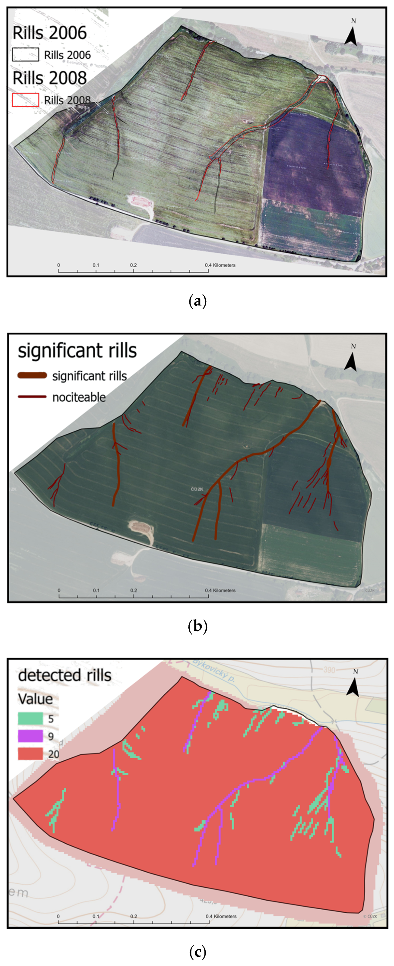
2.4. Field-Scale Rill Flow Validation—A Case Study
3. Results
3.1. Model Calibration and Sensitivity
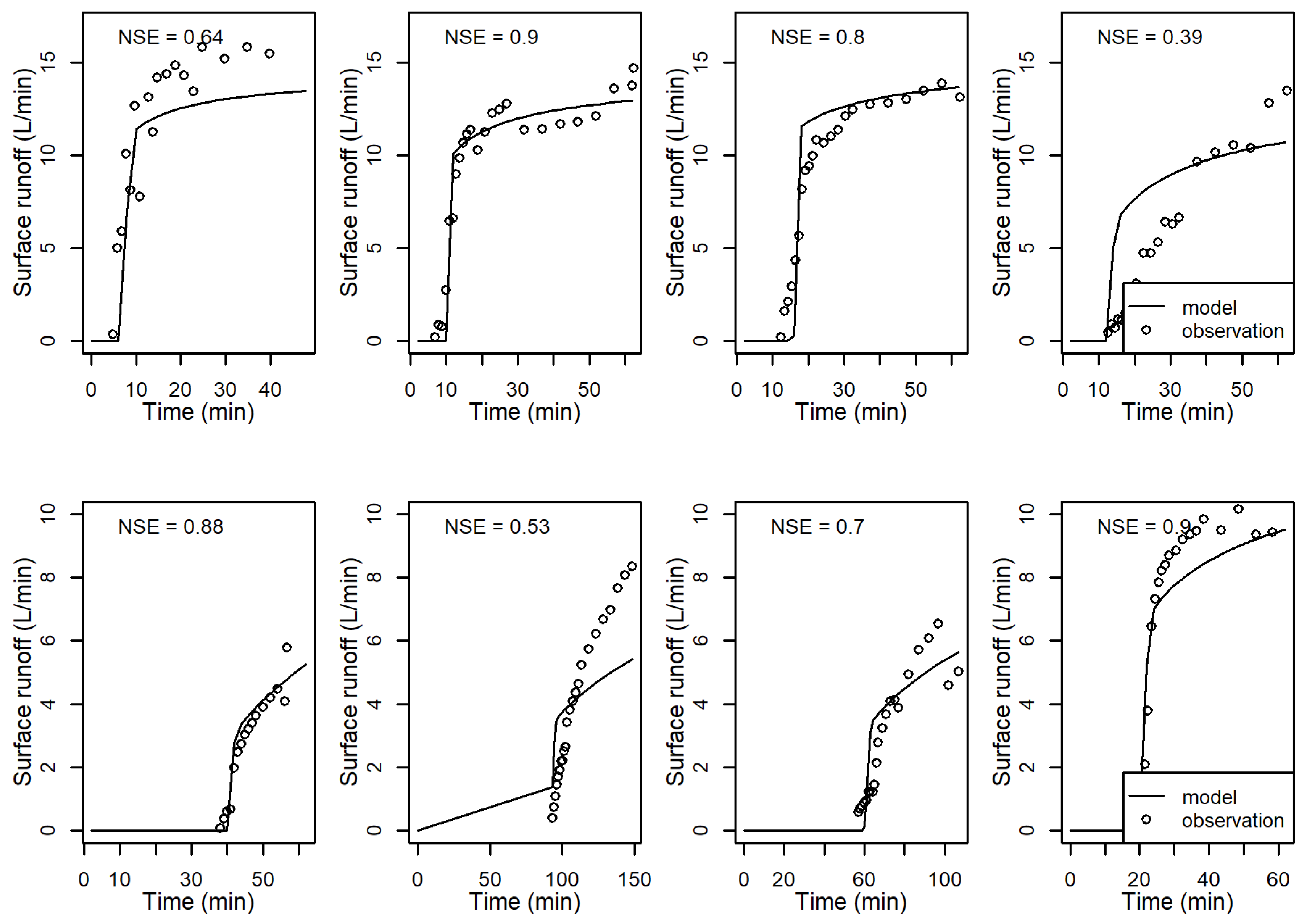
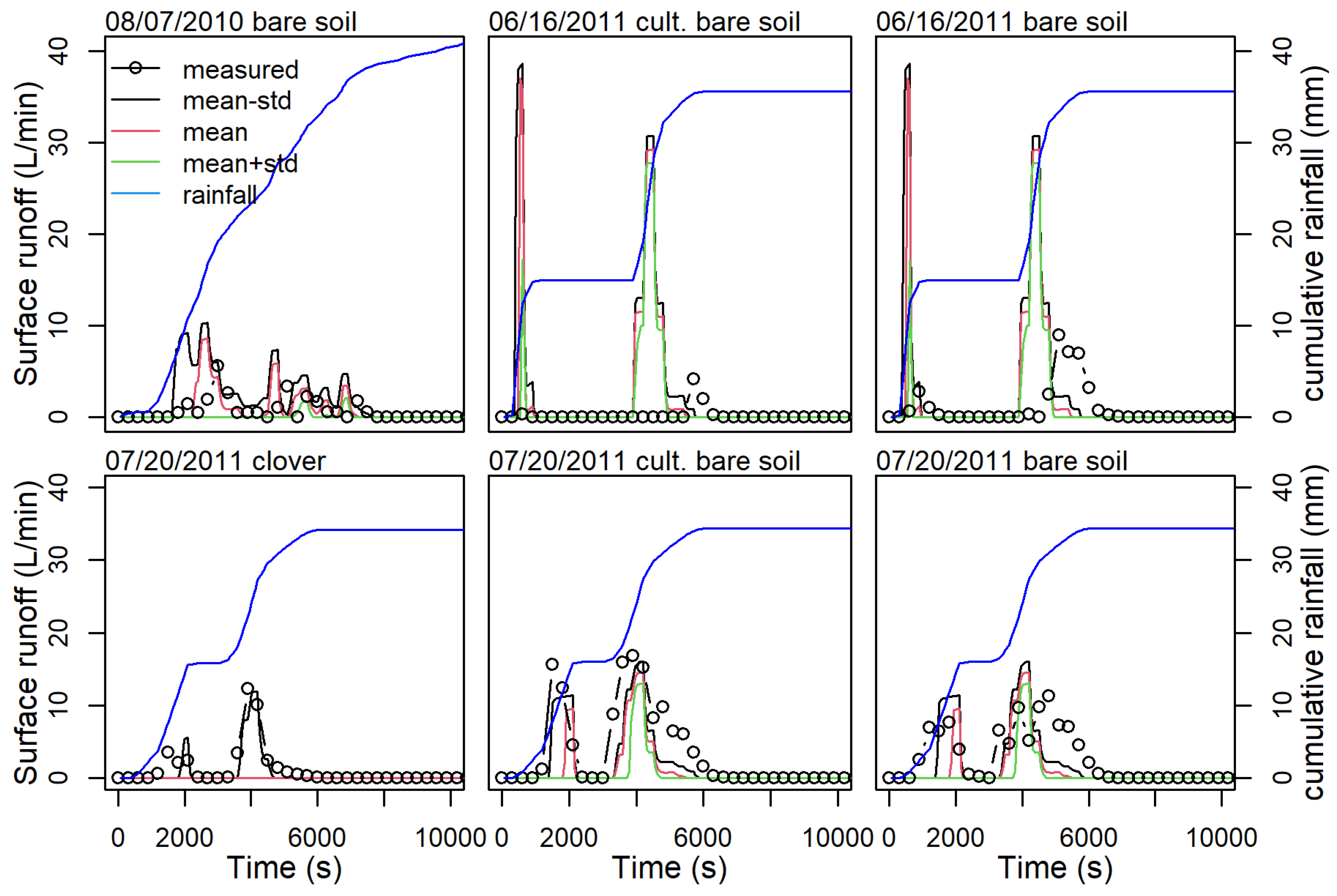
3.2. Model Validation—Plot Scale Sheet Flow
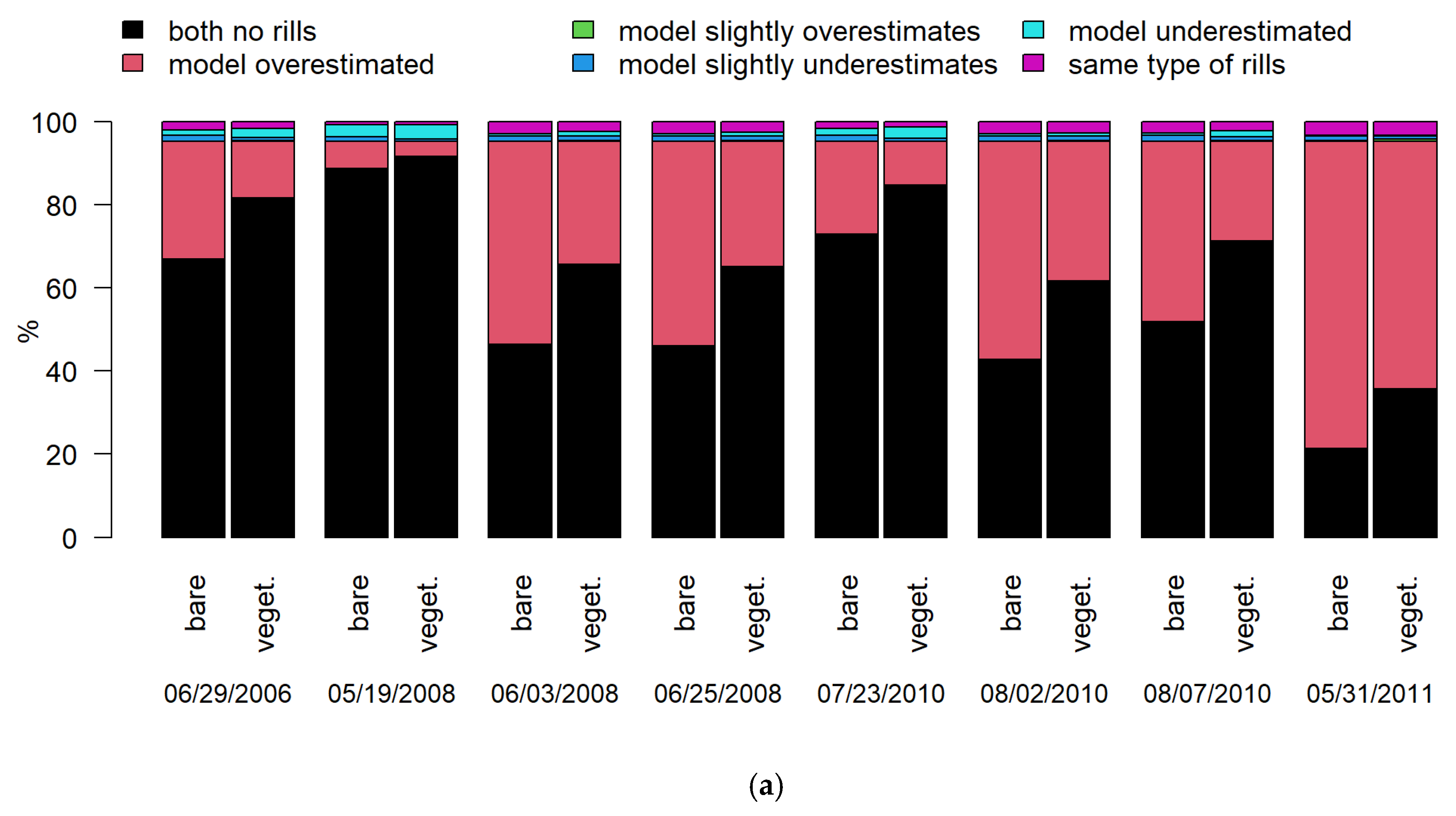
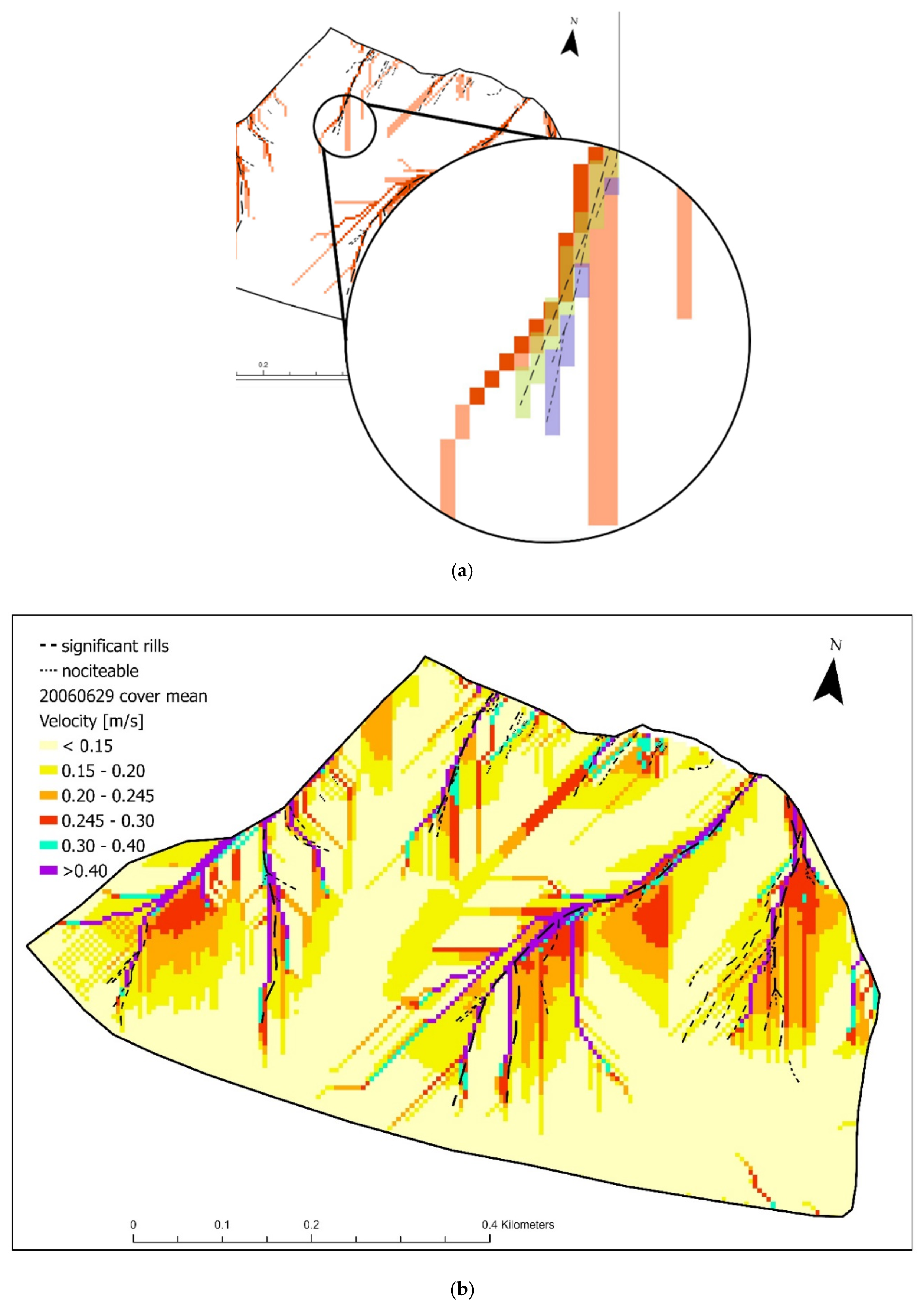
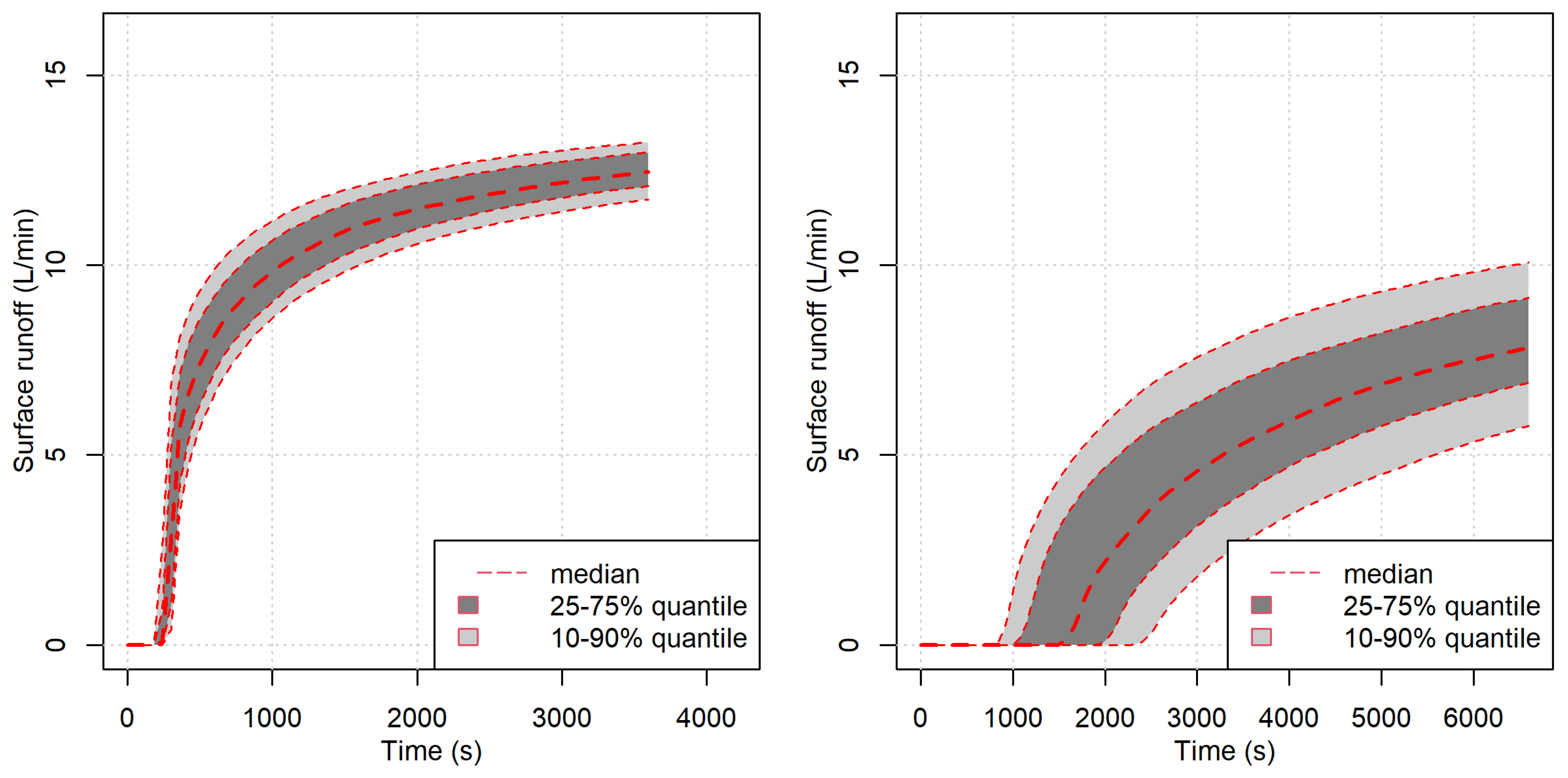
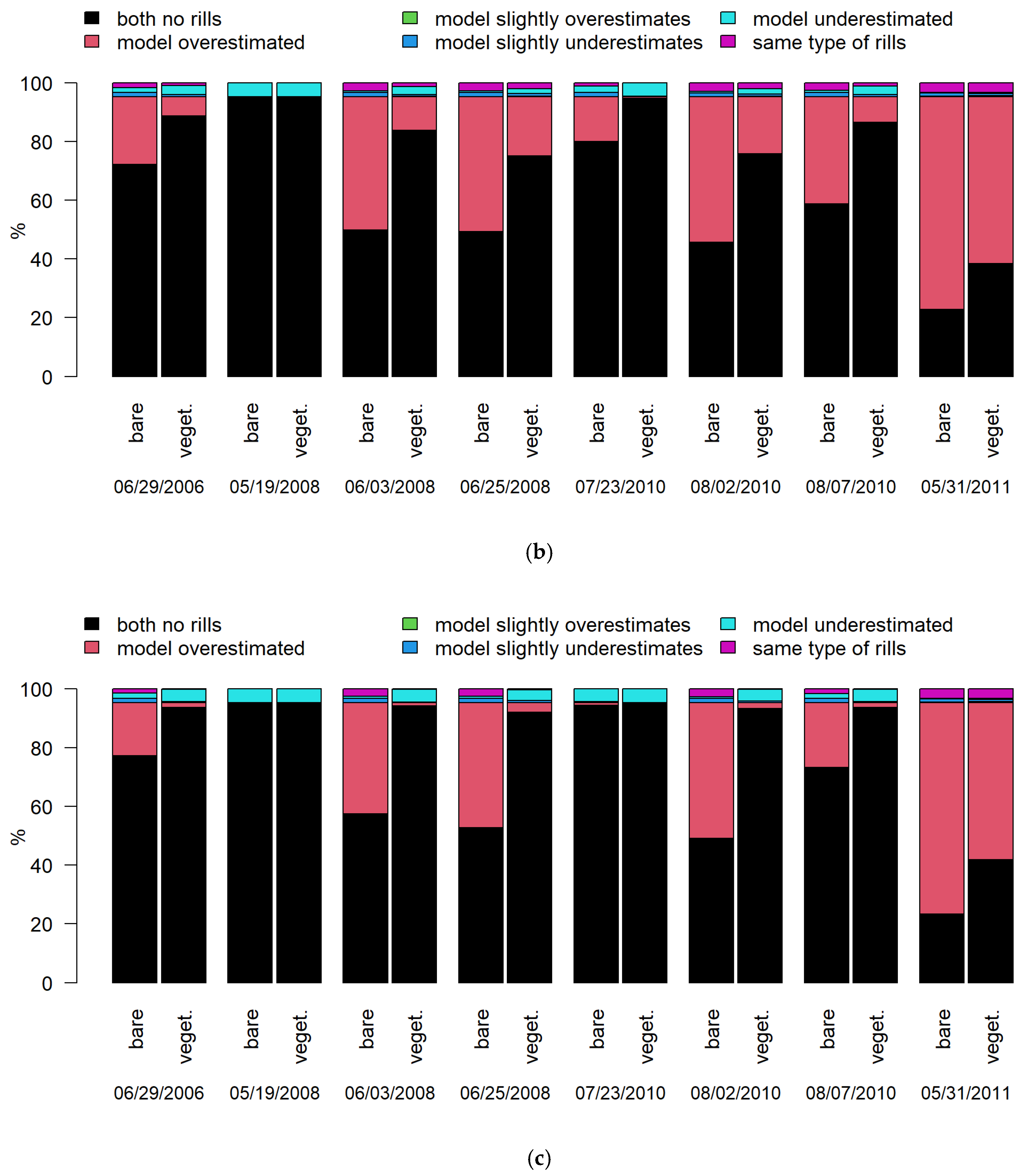
3.3. Model Validation—Field Scale Rill Flow
4. Discussion
4.1. Plot-Scale Sheet Flow Calibration and Validation
4.2. Field-Scale Rill Flow Validation—A Case Study
5. Conclusions
Author Contributions
Funding
Institutional Review Board Statement
Informed Consent Statement
Data Availability Statement
Acknowledgments
Conflicts of Interest
References
- Carpenter, S.R.; Caraco, N.F.; Correll, D.L.; Howarth, R.W.; Sharpley, A.N.; Smith, V.H. Nonpoint pollution of surface waters with phosphorus and nitrogen. Ecol. Appl. 1998, 8, 559–568. [Google Scholar] [CrossRef]
- Probst, J.L. Nitrogen and phosphorus exportation in the Garonne Basin (France). J. Hydrol. 1985, 76, 281–305. [Google Scholar] [CrossRef]
- Boardman, J.; Poesen, J. Soil Erosion in Europe; John Wiley & Sons, Ltd.: Chichester, UK, 2006; Volume 143. [Google Scholar]
- Renard, K.G.; Foster, G.R.; Weesies, G.A.; Porter, J.P. RUSLE: Revised universal soil loss equation. J. Soil. Water Conserv. 1991, 46, 30–33. [Google Scholar]
- Taylor, C.; Al-Mashidani, G.; Davis, J.M. A finite element approach to watershed runoff. J. Hydrol. 1974, 21, 231–246. [Google Scholar] [CrossRef]
- Goodrich, D.C.; Woolhiser, D.A.; Keefer, T.O. Kinematic routing using finite elements on a triangular irregular network. Water Resour. Res. 1991, 27, 995–1003. [Google Scholar] [CrossRef]
- MacArthur, R.C.; de Vries, J.J. Introduction and Application of Kinematic Wave Routing Techniques Using HEC-1; Technical reports; Hydrologic Engineering Center, U.S. Army, Corps of Engineers: Davis, CA, USA, 1993; p. 53. [Google Scholar]
- Jain, M.K.; Kothyari, U.C.; Raju, K.G.R. A GIS based distributed rainfall--runoff model. J. Hydrol. 2004, 299, 107–135. [Google Scholar] [CrossRef]
- Abbott, M.B.; Bathurst, J.C.; Cunge, J.A.; O’connell, P.E.; Rasmussen, J. An introduction to the European Hydrological System—Systeme Hydrologique Europeen,‘SHE’, 2: Structure of a physically-based, distributed modelling system. J. Hydrol. 1986, 87, 61–77. [Google Scholar] [CrossRef]
- Julien, P.Y.; Saghafian, B.; Ogden, F.L. Raster-Based Hydrologic Modeling of Spatially-Varied Surface Runoff. JAWRA J. Am. Water Resour. Assoc. 1995, 31, 523–536. [Google Scholar] [CrossRef]
- Flanagan, D.C.; Elliott, W.J.; Frankenberger, J.R.; Huang, C. WEPP model applications for evaluations of best management practices. In Proceedings of the 16th Congress of the International Soil Conservation Organization, Santiago, Chile, 8–12 November 2010. [Google Scholar]
- USDA. USDA Agricultural Research Service. 2019. Available online: www.ars.usda.gov (accessed on 1 January 2022).
- Von Werner, M. GIS-orientierte Methoden der Digitalen Reliefanalyse zur Modellierung von Bodenerosion in Kleinen Einzugsgebieten. Ph.D. Thesis, Freie Universität Berlin, Berlin, Germany, 1995. [Google Scholar]
- Manning, R. On the flow of water in open channels and pipes. Trans. Inst. Civ. Eng. Irel. 1891, 20, 161–207. [Google Scholar]
- Singh, V.P. Accuracy of kinematic wave and diffusion wave approximations for space independent flows. Hydrol. Process. 1994, 8, 45–62. [Google Scholar] [CrossRef]
- Moramarco, T.; Singh, V.P. Accuracy of kinematic wave and diffusion wave for spatial-varying rainfall excess over a plane. Hydrol. Process. 2002, 16, 3419–3435. [Google Scholar] [CrossRef]
- Kavka, P.; Devaty, J.; Vlacilova, M.; Krasa, J.; Dostal, T. Comparison of soil erosion rills identification by mathematical models and aerial photographs. In Proceedings of the 14th SGEM GeoConference on Informatics, Geoinformatics and Remote Sensing, Albena, Bulgaria, 19–25 June 2014; Volume 1, pp. 521–528. [Google Scholar]
- Holý, M. Vztahy Mezi Povrchovým Odtokem a Transportem Živin v Povodí Vodárenských Nádrží; dílčí zpráva vzkumného ústavu VI-4-15/01-03; Czech Technical University in Prague: Prague, Czech Republic, 1984. [Google Scholar]
- Vrána, K.; Váška, J.; Dostál, T. Smoderp—Uživatelský Manuál; Czech Technical University in Prague: Prague, Czech Republic, 1996. [Google Scholar]
- Dostál, T.; Váška, J.; Vrána, K. SMODERP—A Simulation Model of Overland Flow and Erosion Processes. In Soil Erosion: Application of Physically Based Models; Schmidt, J., Ed.; Springer: Berlin/Heidelberg, Germany, 2000; pp. 135–161. [Google Scholar] [CrossRef]
- Kavka, P. Kalibrace a Validace Modelu Smoderp. Ph.D. Thesis, Czech Technical University in Prague, Prague, Czech, 2011. [Google Scholar]
- Wischmeier, W.H.; Smith, D.D. Predicting Rainfall Erosion Losses—A Guide to Conservation Planning; Agricultur. U.S. Department of Agriculture: Washington, DC, USA, 1978. [Google Scholar]
- Marques, M.J.; Bienes, R.; Jiménez, L.; Pérez-Rodríguez, R. Effect of vegetal cover on runoff and soil erosion under light intensity events. Rainfall simulation over USLE plots. Sci. Total Environ. 2007, 378, 161–165. [Google Scholar] [CrossRef] [PubMed]
- McGregor, K.C.; Mutchler, C.K. Soil Loss from Conservation Tillage for Sorghum. Trans. ASAE 1992, 35, 1841–1845. [Google Scholar] [CrossRef]
- Bryan, R.; de Ploey, J. Comparability of soil erosion measurements with different laboratory rainfall simulators. Catena. Suppl. 1983, 4, 33–56. [Google Scholar]
- De Ploey, J. Rainfall Simulation Runoff and Soil Erosion; Catena Supplements, 4; Schweizerbart: Stuttgart, Germany, 1983; p. 214. [Google Scholar]
- Cerdà, A.; Jurgensen, M.F. Ant mounds as a source of sediment on citrus orchard plantations in eastern Spain. A three-scale rainfall simulation approach. CATENA 2011, 85, 231–236. [Google Scholar] [CrossRef]
- Nichols, M.L.; Sexton, H.D. A method of studying soil erosion. Agric. Eng. 1932, 13, 101–103. [Google Scholar]
- NIED. Large-Scale Rainfall Simulator; Experimental Facilities; The National Research Institute for Earth Science and Disaster Resilience (NIED): Tsukuba, Japan, 2021; Available online: www.bosai.go.jp (accessed on 1 January 2022).
- Iserloh, T.; Ries, J.; Arnáez, J.; Boix-Fayos, C.; Butzen, V.; Cerdà, A.; Echeverría, M.; Fernández-Gálvez, J.; Fister, W.; Geißler, C.; et al. European small portable rainfall simulators: A comparison of rainfall characteristics. CATENA 2013, 110, 100–112. [Google Scholar] [CrossRef] [Green Version]
- Gires, A.; Bruley, P.; Ruas, A.; Schertzer, D.; Tchiguirinskaia, I. Disdrometer measurements under Sense-City rainfall simulator. Earth Syst. Sci. Data 2020, 12, 835–845. [Google Scholar] [CrossRef] [Green Version]
- Zumr, D.; Mützenberg, D.V.; Neumann, M.; Jeřábek, J.; Laburda, T.; Kavka, P.; Johannsen, L.L.; Zambon, N.; Klik, A.; Strauss, P.; et al. Experimental Setup for Splash Erosion Monitoring—Study of Silty Loam Splash Characteristics. Sustainability 2019, 12, 157. [Google Scholar] [CrossRef] [Green Version]
- Edwards, L.M.; Burney, J.R. Soil Erosion Losses Under Freeze/Thaw and Winter Ground Cover Using a Laboratory Rainfall Simulator. Can. Agric. Eng. 1987, 29, 109–115. [Google Scholar]
- Davidova, T.; Dostal, T.; David, V.; Strauss, P. Determining the protective effect of agricultural crops on the soil erosion process using a field rainfall simulator. Plant Soil Environ. 2016, 61, 109–115. [Google Scholar] [CrossRef] [Green Version]
- Maugnard, A.; Cordonnier, H.; Degre, A.; Demarcin, P.; Pineux, N.; Bielders, C.L. Uncertainty assessment of ephemeral gully identification, characteristics and topographic threshold when using aerial photographs in agricultural settings. Earth Surf. Process. Landf. 2014, 39, 1319–1330. [Google Scholar] [CrossRef]
- Eltner, A.; Baumgart, P.; Maas, H.-G.; Faust, D. Multi-temporal UAV data for automatic measurement of rill and interrill erosion on loess soil. Earth Surf. Process. Landf. 2014, 40, 741–755. [Google Scholar] [CrossRef]
- Fulajtár, E. Identification of severely eroded soils from remote sensing data tested in Rišňovce, Slovakia. In Proceedings of the 10th International Soil Erosion Conservation Organization Meeting at Purdue University and the USDA-ARS National Soil Erosion Research Laboratory, Lafayette, LA, USA, 24–29 May 1999. [Google Scholar]
- Wang, T.; He, F.; Zhang, A.; Gu, L.; Wen, Y.; Jiang, W.; Shao, H. A Quantitative Study of Gully Erosion Based on Object-Oriented Analysis Techniques: A Case Study in Beiyanzikou Catchment of Qixia, Shandong, China. Sci. World J. 2014, 2014, 1–11. [Google Scholar] [CrossRef]
- Báčová, M.; Krása, J.; Devátý, J.; Kavka, P. A GIS method for volumetric assessments of erosion rills from digital surface models. Eur. J. Remote Sens. 2018, 52, 96–107. [Google Scholar] [CrossRef] [Green Version]
- Kaiser, A.; Neugirg, F.; Rock, G.; Müller, C.; Haas, F.; Ries, J.; Schmidt, J. Small-Scale Surface Reconstruction and Volume Calculation of Soil Erosion in Complex Moroccan Gully Morphology Using Structure from Motion. Remote Sens. 2014, 6, 7050–7080. [Google Scholar] [CrossRef] [Green Version]
- Vinci, A.; Brigante, R.; Todisco, F.; Mannocchi, F.; Radicioni, F. Measuring rill erosion by laser scanning. CATENA 2015, 124, 97–108. [Google Scholar] [CrossRef]
- Bauer, T.; Strauss, P.; Grims, M.; Kamptner, E.; Mansberger, R.; Spiegel, H. Long-term agricultural management effects on surface roughness and consolidation of soils. Soil Tillage Res. 2015, 151, 28–38. [Google Scholar] [CrossRef]
- Laburda, T.; Krása, J.; Zumr, D.; Devátý, J.; Vrána, M.; Zambon, N.; Johannsen, L.L.; Klik, A.; Strauss, P.; Dostál, T. SfM-MVS Photogrammetry for Splash Erosion Monitoring under Natural Rainfall. Earth Surf. Process. Landf. 2021, 46, 1067–1082. [Google Scholar] [CrossRef]
- Philip, J.R. The theory of infiltration: 1. The infiltration equation and its solution. Soil Sci. 1975, 83, 345–357. [Google Scholar] [CrossRef]
- O’Callaghan, J.F.; Mark, D.M. The extraction of drainage networks from digital elevation data. Comput. Vis. Graph. Image Process. 1984, 28, 323–344. [Google Scholar] [CrossRef]
- Zhang, W.; Cundy, T.W. Modeling of two-dimensional overland flow. Water Resour. Res. 1989, 25, 2019–2035. [Google Scholar] [CrossRef]
- Esteves, M.; Faucher, X.; Galle, S.; Vauclin, M. Overland flow and infiltration modelling for small plots during unsteady rain: Numerical results versus observed values. J. Hydrol. 2000, 228, 265–282. [Google Scholar] [CrossRef]
- Šilhavý, J.; Čada, V. New automatic accuracy evaluation of altimetry data: DTM 5G compared with ZABAGED®altimetry. Lect. Notes Geoinf. Cartogr. 2015, 211, 225–236. [Google Scholar] [CrossRef]
- Tolasz, R.; Míková, T.; Valeriánová, A.; Voženílek, V. Atlas of the Czech Climate; Czech Hydrometeorological Institute, Palacký University Olomouc: Prague, Czech Republic, 2007; p. 255. [Google Scholar]
- Kašpar, M.; Bližňák, V.; Hulec, F.; Müller, M. High-resolution spatial analysis of the variability in the subdaily rainfall time structure. Atmos. Res. 2020, 248, 105202. [Google Scholar] [CrossRef]
- Muller, M.; Kašpar, M.; Bližvnák, V.; Kavka, P. Precipitation intensity during heavy rains in various altitudes. In Proceedings of the Rainfall in Urban and Natural Systems. 10th International Workshop on Precipitation in Urban Areas, Pontresina, Switzerland, 1–5December 2015. [Google Scholar] [CrossRef]
- Sokol, Z.; Bližňák, V. Areal distribution and precipitation–altitude relationship of heavy short-term precipitation in the Czech Republic in the warm part of the year. Atmos. Res. 2009, 94, 652–662. [Google Scholar] [CrossRef]
- Báčová, M.; Krása, J.; Vláčilová, M. Application of historical and recent aerial imagery in monitoring water erosion occurrences in Czech highlands. Soil Water Res. 2016, 11, 267–276. [Google Scholar] [CrossRef] [Green Version]
- Nash, J.E.; Sutcliffe, J.V. River flow forecasting through conceptual models part I—A discussion of principles. J. Hydrol. 1970, 10, 282–290. [Google Scholar] [CrossRef]
- Mishra, S.K.; Tyagi, J.V.; Singh, P.V.P. Comparison of infiltration models. Hydrol. Process. 2003, 17, 2629–2652. [Google Scholar] [CrossRef]
- Ewen, J. Hydrograph matching method for measuring model performance. J. Hydrol. 2011, 408, 178–187. [Google Scholar] [CrossRef]
- Heckmann, T.; Vericat, D. Computing spatially distributed sediment delivery ratios: Inferring functional sediment connectivity from repeat high-resolution digital elevation models. Earth Surf. Process. Landf. 2018, 43, 1547–1554. [Google Scholar] [CrossRef]
- Brunton, D.A.; Bryan, R.B. Rill network development and sediment budgets. Earth Surf. Process. Landf. 2000, 25, 783–800. [Google Scholar] [CrossRef]
- Wu, S.; Chen, L. Modeling Soil Erosion With Evolving Rills on Hillslopes. Water Resour. Res. 2020, 56, 1–18. [Google Scholar] [CrossRef]
- Bennett, S.J.; Gordon, L.M.; Neroni, V.; Wells, R.R. Emergence, persistence, and organization of rill networks on a soil-mantled experimental landscape. Nat. Hazards 2015, 79, 7–24. [Google Scholar] [CrossRef]
- Žížala, D.; Minařík, R.; Beitlerová, H.; Juřicová, A.; Skála, J.; Rojas, J.R.; Penížek, V.; Zádorová, T. High-Resolution Soil Property Maps from Digital Soil Mapping Methods, Czech Republic. SSRN Electron. J. 2021, 53. [Google Scholar] [CrossRef]
- Ou, X.; Hu, Y.; Li, X.; Guo, S.; Liu, B. Advancements and challenges in rill formation, morphology, measurement and modeling. Catena 2021, 196, 104932. [Google Scholar] [CrossRef]


| Measured | Modelled | Sum of Measured and Modelled Values | Interpretation Code | |||
|---|---|---|---|---|---|---|
| Value of Pixel | Rill Type | Value of Pixel | Rill Type | |||
| 5 | SR | 0 | NoRill | 5 | 1 | model underestimates |
| 9 | NR | 0 | NoRill | 9 | 2 | model underestimates |
| 20 | NoRill | 1 | SR | 21 | 10 | model overestimates |
| 20 | NoRill | 2 | NR | 22 | 20 | model overestimates |
| 5 | SR | 1 | SR | 6 | 101 | same type of rill |
| 5 | SR | 2 | NR | 7 | 102 | model slightly underestimates |
| 9 | NR | 1 | SR | 10 | 201 | model slightly overestimates |
| 9 | NR | 2 | NR | 11 | 202 | same type of rill |
| 20 | NoRill | 0 | NoRill | 20 | NODATA | no rill |
| Bare Soil | Vegetation | |||
|---|---|---|---|---|
| Rainfall | Mean | STD | Mean | STD |
| rainfall intensity (mm/hour) | 59.7 | 2.0 | 61.3 | 2.6 |
| rainfall duration (mins) | 63.7 | 0.9 | 109.8 | 42.0 |
| Soil | ||||
| Hydraulic conductivity (m/s) | 7.02 × 10⁻⁷ | 5.87 × 10⁻⁷ | 1.53 × 10⁻⁶ | 1.47 × 10⁻⁶ |
| Sorptivity (m/s1/2) | 3.58 × 10⁻⁴ | 1.01 × 10⁻⁴ | 1.11 × 10⁻³ | 3.71 × 10⁻⁴ |
| Veg. parameters | ||||
| Leaf area index (-) | 0 | 0 | 0.200 | 0.184 |
| Potential interception (mm) | 0 | 0 | 0.501 | 0.499 |
| Surface characteristics | ||||
| surface retention (mm) | 4.67 | 2.49 | 3.35 | 1.33 |
| Manning’s roughness (s/m1/3) | 3.33 × 10⁻² | 2.36 × 10⁻³ | 8.38 × 10⁻² | 2.81 × 10⁻² |
| Surface flow equation | ||||
| b (-) | 1.79 | * | 1.79 | * |
| Y (-) | 0.69 | * | 0.69 | * |
| X (-) | 9.33 | 0.94 | 10.00 | * |
| Date | Surface | Correlation Coefficient | NSE | ||||
|---|---|---|---|---|---|---|---|
| MEAN − STD | MEAN | MEAN + STD | MEAN − STD | MEAN | MEAN + STD | ||
| 7 August 2010 | bare | 0.52 | 0.48 | 0.09 | −4.47 | −1.12 | −0.16 |
| 16 June 2011 | bare (cultivated) | 0.04 | 0.02 | 0 | 0.75 | 0.47 | 0.23 |
| 16 June 2011 | bare | 0.1 | 0.05 | 0.02 | 0.39 | 0.20 | 0.03 |
| 20 July 2011 | vegetated (clover) | 0.88 | No modelled surface runoff | 0.77 | No modelled surface runoff | ||
| 20 July 2011 | bare (cultivated) | 0.85 | 0.65 | 0.59 | 0.70 | 0.35 | 0.25 |
| 20 July 2011 | bare | 0.67 | 0.49 | 0.42 | 0.19 | 0.03 | −0.01 |
| Date | Time (h) | Rainfall Duration (min) | Total Rain (mm) |
|---|---|---|---|
| 29 June 2006 | 11 | 950 | 83.1 |
| 19 May 2008 | 10 | 500 | 19.3 |
| 3 June 2008 | 8 | 100 | 15.2 |
| 25 June 2008 | 17 | 100 | 20.1 |
| 23 July 2010 | 18 | 230 | 20.2 |
| 2 August 2010 | 20 | 210 | 25.4 |
| 7 August 2010 | 8 | 970 | 71.2 |
| 31 May 2011 | 15 | 50 | 29.5 |
Publisher’s Note: MDPI stays neutral with regard to jurisdictional claims in published maps and institutional affiliations. |
© 2022 by the authors. Licensee MDPI, Basel, Switzerland. This article is an open access article distributed under the terms and conditions of the Creative Commons Attribution (CC BY) license (https://creativecommons.org/licenses/by/4.0/).
Share and Cite
Kavka, P.; Jeřábek, J.; Landa, M. SMODERP2D—Sheet and Rill Runoff Routine Validation at Three Scale Levels. Water 2022, 14, 327. https://doi.org/10.3390/w14030327
Kavka P, Jeřábek J, Landa M. SMODERP2D—Sheet and Rill Runoff Routine Validation at Three Scale Levels. Water. 2022; 14(3):327. https://doi.org/10.3390/w14030327
Chicago/Turabian StyleKavka, Petr, Jakub Jeřábek, and Martin Landa. 2022. "SMODERP2D—Sheet and Rill Runoff Routine Validation at Three Scale Levels" Water 14, no. 3: 327. https://doi.org/10.3390/w14030327
APA StyleKavka, P., Jeřábek, J., & Landa, M. (2022). SMODERP2D—Sheet and Rill Runoff Routine Validation at Three Scale Levels. Water, 14(3), 327. https://doi.org/10.3390/w14030327