Article

A Low-Cost Wireless Sensor for Real-Time Monitoring of Water Level in Lowland Rice Field under Alternate Wetting and Drying Irrigation

by
Kristelle Marie S. Dela Cruz
1,*,
Victor B. Ella
1,*,
Delfin C. Suministrado
2,
Gamiello S. Pereira
1 and
Edzel S. Agulto
1
1
Land and Water Resources Engineering Division, Institute of Agricultural and Biosystems Engineering, College of Engineering and Agro-Industrial Technology, University of the Philippines Los Baños, Los Banos 4031, Philippines
2
Agribiosystems, Machinery and Power Engineering Division, Institute of Agricultural and Biosystems Engineering, College of Engineering and Agro-Industrial Technology, University of the Philippines Los Baños, Los Banos 4031, Philippines
*
Authors to whom correspondence should be addressed.
Water 2022, 14(24), 4128; https://doi.org/10.3390/w14244128
Submission received: 19 November 2022 / Revised: 9 December 2022 / Accepted: 15 December 2022 / Published: 19 December 2022
(This article belongs to the Special Issue Advances in Sustainable Agriculture Progress under Climate Change)

Abstract

:
The use of wireless sensors for real-time monitoring of field water level would greatly facilitate the application of alternate wetting and drying (AWD), an irrigation water management technique proven to result to significant water savings and reduced methane emissions in lowland rice production systems. However, most of the commercially available wireless sensors are generally costly. This study developed a low-cost wireless sensor that can perform real-time monitoring of water depth and surface temperature in lowland rice fields under an AWD irrigation regime. The sensor is composed mainly of an ultrasonic depth sensor, a waterproof temperature sensor, a humidity sensor, and a Wi-Fi-enabled microcontroller enclosed in a PVC cap that can be mounted in AWD pipes. The sensor was tested under laboratory, pseudo-field conditions and actual field conditions. Results showed a relatively high degree of agreement between sensor and manual measurements of water depth under all testing conditions, with the error ranging from only 5.2% to 6.6% and RMSE of 5.0 mm to 13.5 mm. The performance of the low-cost sensor also proved to be comparable with that of the high-end sensor, exhibiting practically similar measurement accuracy and higher precision. The wireless sensor developed in this study can provide a low-cost alternative to the high-cost and high-end sensors and other commercially available counterparts for efficient irrigation water management in lowland crop production systems during water-scarce conditions induced by climate change and climate variability.

1. Introduction

Lowland rice irrigation systems are known to consume a considerable amount of freshwater resources, comprising a 34–43% share of the world’s total irrigation water and 24–30% of the world’s developed freshwater resources [1]. Rice cultivation is also identified as a significant source of methane emissions (CH4) due to anaerobic process brought about by its flooding nature, accounting for about 10% of the global non-CO2 emissions in agriculture [2]. In the face of climate uncertainties and hydrological extremes, it is therefore imperative that we adopt efficient water management practices in countering water scarcity issues to carry on with the production of food staple of about half of the global population [3]. Among the many alternative water saving techniques developed is the alternate wetting and drying (AWD) technology, a form of irrigation management where the field water level is being brought to a water level threshold in the soil subsurface, with 15 cm being the safe maximum, before triggering another irrigation event [4]. The AWD has been proven to be effective in reducing irrigation water consumption without significant yield compensations [5,6,7]. It was also reported to reduce CH4 emissions [8,9,10,11,12,13,14], and is therefore considered as a promising option in mitigating global warming potential from rice cultivation.
Aside from the increased water productivity and environmental benefits, the application of the AWD irrigation has also been known to reduce labor requirements with less frequent irrigation [15], although the tradeoff brings about the challenge in constantly monitoring the field water level, often done manually, to ensure that the level will never get below the safe threshold. The advent of sensor technology and its application in irrigation has greatly alleviated this challenge by enabling remote monitoring. Recent developments in real-time monitoring of field water level have aided farmers and researchers alike in coming up with sound and efficient irrigation water management plans and decisions.
Wireless sensors applicable for irrigation water management in rice fields have evolved in recent years. Most of the previously developed sensors are capable of monitoring field water level [16,17,18,19], together with soil moisture [20,21] and other climatic variables [22,23]. The developed technologies greatly vary in the usage of sensor types, communication protocols, and system architecture. While a number of wireless sensors have been developed, most of them are costly, especially those that make use of high-end hardware and cutting-edge technologies. Other sensor development studies of the low-end type, on the other hand, did not include rigorous sensor testing or published sensor performance results, thus failing to unravel potential problems associated with field implementation. Some other sensors are not user-friendly such that widespread adoption may become a challenge. With the availability of open-source software, different sensor types and wireless communication protocols, the opportunities remain vast in coming up with a variety of options for affordable, user-friendly, and effective monitoring systems for real-time water information.
This study aimed to develop an alternative to existing costly sensors for real-time monitoring of water level in lowland crop production systems employing AWD. This paper presents the details of the sensor development and rigorous testing under laboratory, pseudo-field, and actual field conditions. Ultimately, the sensors developed in this study are intended to facilitate the wider application of AWD in lowland crop production systems in order to address issues of water scarcity and inequitable water distribution induced by climate change and climate variability.

2. Materials and Methods

2.1. Sensor Development
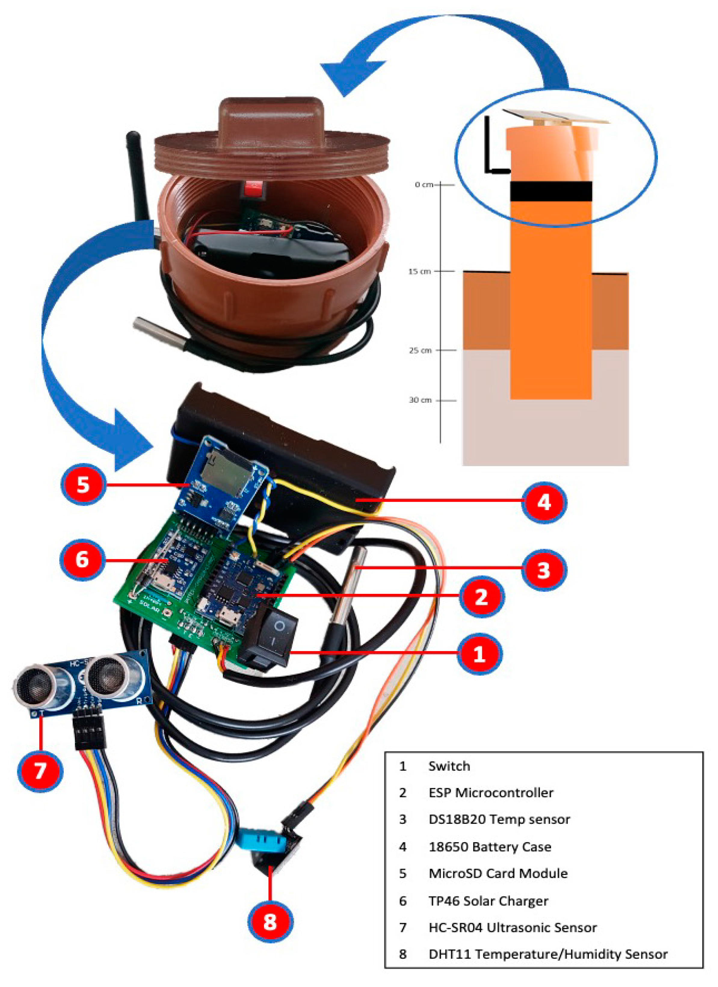
2.1.1. Hardware

The sensor unit was enclosed in a 4″-diameter PVC cap that was mounted on top of a 4″-diameter AWD pipe. The low-cost sensor is composed mainly of four sensor modules: HC-SR04 ultrasonic distance sensor, DS18B20 waterproof temperature sensor, DHT11 temperature/humidity sensor, and the microSD card adapter module. Data from the sensor modules are integrated by the ESP8266 microcontroller which sends data to the online database through Wi-Fi. The sensor unit was also equipped with two Li ion batteries, a solar charger, and two mini solar panels. Figure 1 shows the connection of the sensor circuitry.
For the microcontroller of the circuit, the Wemos D1 mini Pro was used. It is Arduino-compatible and has 11 digital input/output (I/O) pins. It has a built-in ESP8266 Wi-Fi module that enables the microcontroller to connect to the Wi-Fi network. With this, the sensor data can be accessed via the cloud. A microSD card adapter module was also integrated into the circuit to contain data in a text file for manual retrieval. The DS18B20 waterproof temperature sensor was used to monitor the soil surface temperature that could handle the field’s day-to-night temperature fluctuations very well. The sensor has a 4.7 kΩ resistor connected in parallel between the power cable and data cable for the sensor to work properly. For the measurement of the field water level, the HC-SR04 ultrasonic distance sensor was used. Since the microcontroller has an operating voltage of 3.3 V while the distance sensor works on 5 V, voltage dividers were placed in the form of 1.2 KΩ and 2.2 KΩ resistors. This is to ensure that the output voltage coming out from the echo pin is in the voltage level that the microcontroller can safely handle. Additionally, since the Wemos D1 mini Pro board has a very limited number of I/O pins, the distance sensor was configured to perform under a single pin operation with the use of the NewPing library function. Accuracy of distance readings was improved through iterations. For the power source, one TP4056 battery charger was used to charge two 3.7 V–2100 mAh 18650 Li-ion batteries connected in parallel, while two IN5819 diodes were used to prevent backflow current from the batteries to the solar panels. A 180 KΩ resistor was installed between the analogue pin (A0) and 5 V pin to serve as a battery gauge. The voltage readings of the sensor measured from the analogue pin were successfully validated by the multimeter readings. A printed circuit board was designed to interweave the sensor components altogether using less wires. It has also made the entire sensor unit to be compacted, conveniently space-wise for circuit packaging and field deployment. Figure 2 shows the fabricated prototype of the sensor and its intended installation with the AWD pipe. In total, 10 sensors were exclusively tested under different conditions: laboratory, pseudo-field, and actual field. The methodology of the testing process is elaborated in a separate subsection (Sensor Testing).

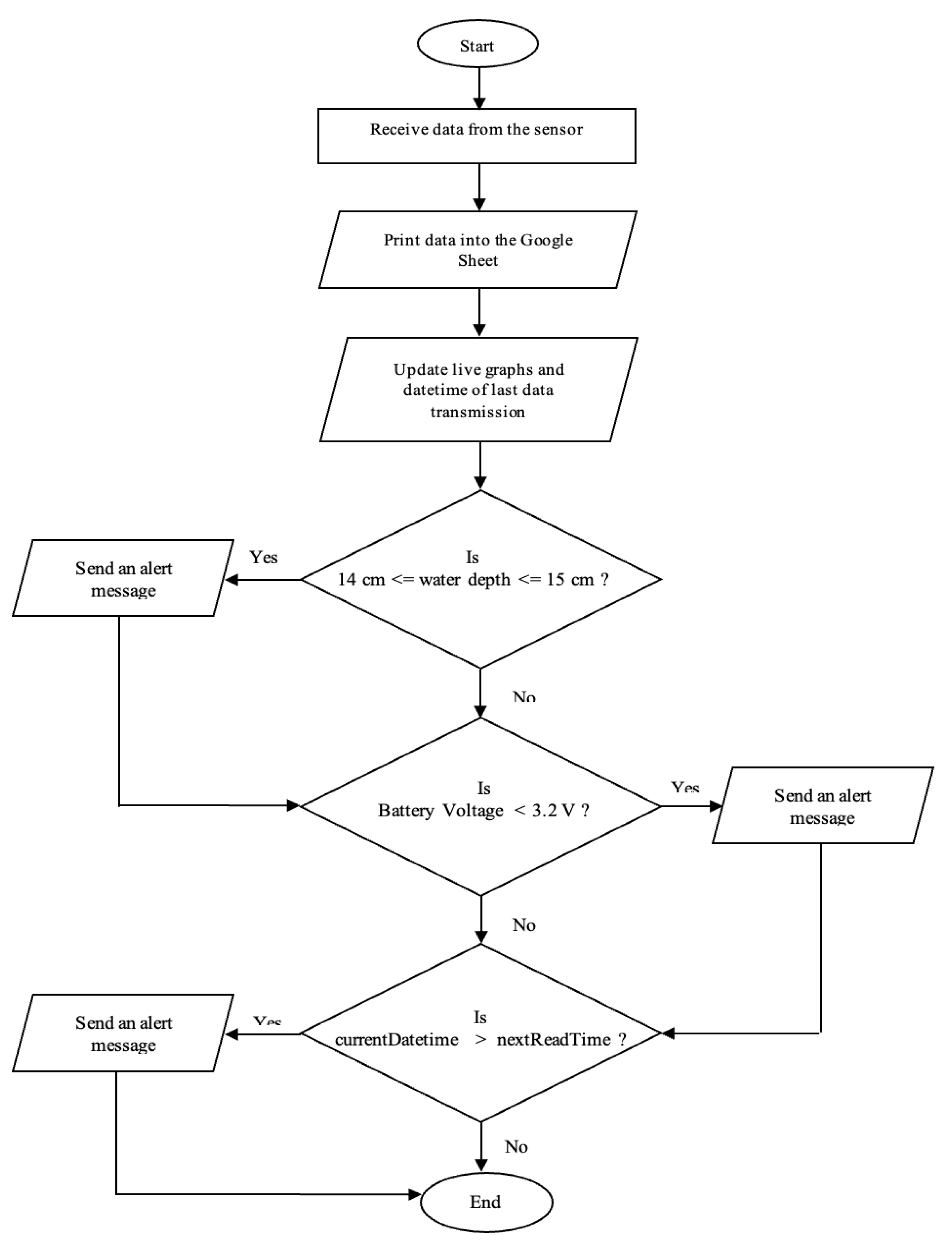
2.1.2. Sensor Programming

Sensor programming was made using the Arduino Integrated Development Environment (IDE). Since the Wemos and Arduino boards have different pinout architecture, adjustments on pin designations were employed to make the Wemos codes work in the Arduino IDE. Necessary libraries were used for programming the different sensor modules.
Scripts were made for offline and online data logging. For every sensor reading, the data are automatically sent to the cloud database and encoded into the text file created into the SD card at the same time. This serves as a backup in case of internet connection failure. With the microSD card adapter, most of the digital pins were used up to establish communication between the microcontroller and the SD card module. This has greatly limited the number of digital sensors that can be integrated in the circuit. Thus, the RX pin, which originally serves for the purpose of serial communication, was converted to function as a digital pin to accommodate DHT11. To save power, the sensors were programmed to be in deep-sleep mode and only read data in one-hour intervals. This was made possible by placing 220 Ω resistor between the D0 and RST microcontroller pins. Figure 3 shows the logic of the sensor operation.

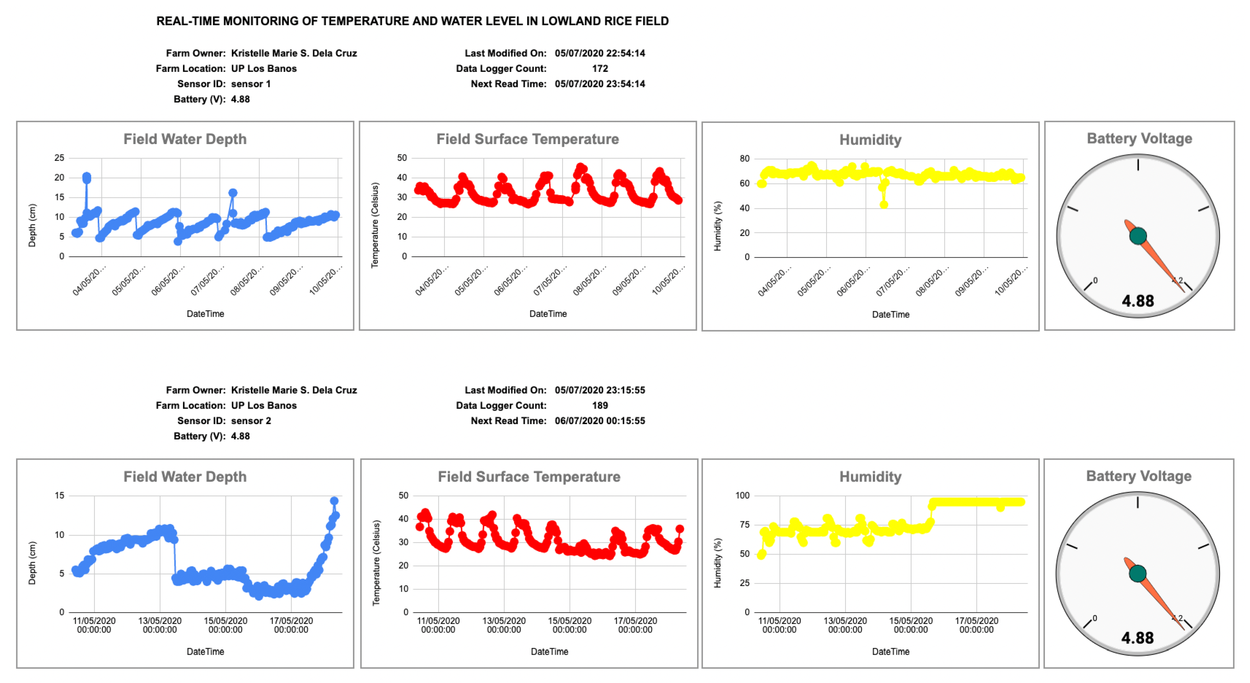
2.1.3. Online Database and Alert Messaging Systems
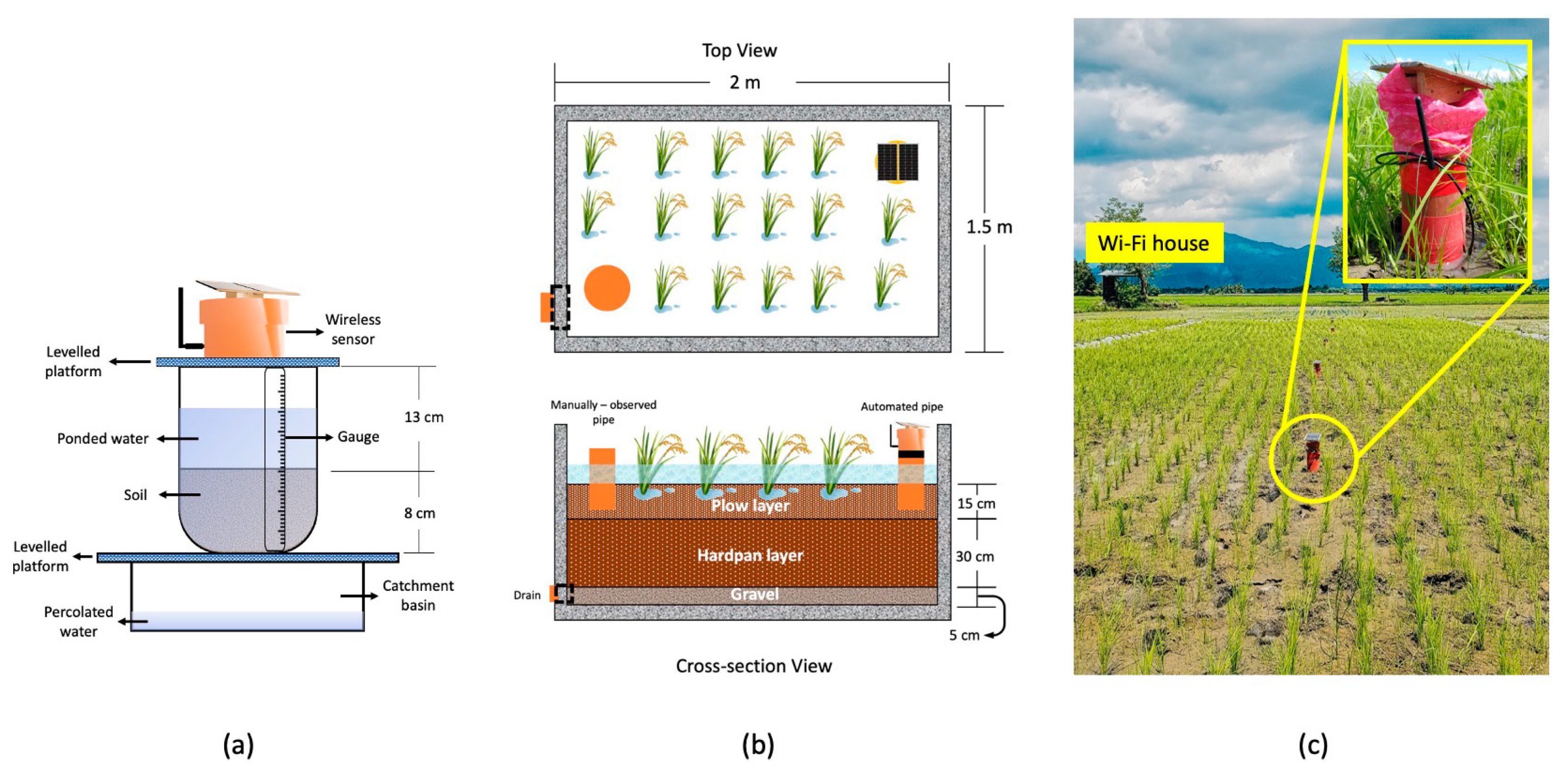
A web app, whose algorithm is shown in Figure 4, was developed using the Google App Script to receive data from the microcontroller. For every sensor reading, the microcontroller automatically sends the sensor data into the cloud. The data are directed into the designated Google Sheet of the end user for remote and real-time monitoring of temperature and water level in the farm. Real-time graphs of field water depth, temperature and humidity were created using the Google Sheet charts, which come along with other important information, such as date and time of data transmission, battery voltage, and total number of data entries in the database. A sample of the dataset is shown in Table A1, while the sample dashboard is shown in Figure 5. Currently, the database can accommodate real-time data from five sensors simultaneously, with each sensor having its own designated logging sheets. It can further be configured according to the number of sensors desired for use.
Aside from the online data management system, an alert messaging scheme was also incorporated in the script to notify the users during emergencies. The alert system is triggered by the following conditions: when the water level is about to reach the safe AWD threshold, thus warning the farmer that the irrigation operation is needed soon; when the battery power is about to run out, thus urging the farmer to replace the batteries; and when the sensor did not send data past its expected reading time, advising the farmer to inspect the sensor on site. When one of the said conditions arises, an email is sent to the end user indicating the type of emergency that happened and the specific actions to be performed. The message also indicates the identification of the sensor that is currently needing attention.
The AWD threshold level exemplified in the code, i.e., 15 cm, is the safe threshold usually adopted in most studies. Since the ultrasonic sensor measures the distance between itself and the target surface, the reference elevation follows the relative height of the sensor from the soil surface where it is being mounted. Thus, necessary adjustments have to be made to properly reflect the safe AWD depth threshold in sensor readings with respect to the soil surface. A 1 cm allowance was also given before the safe AWD threshold to set a grace time period between the time of warning and the supposed irrigation schedule. As for the battery, the voltage threshold was set to 3.2 V. An even lower voltage level may already compromise the sensor performance since the Wemos D1 mini Pro requires a 3.3 V operating voltage. And lastly, the alert system informs the user if a specific sensor has failed to send data beyond its expected reading time. Once a new sensor data has entered the database, the script will log the latest datetime of entry and update the next reading time of the sensor by adding 1 h from the current date and time. After such, the script will evaluate if the current date and time has exceeded the expected reading time of the other sensors in the database. If a sensor has failed to send data for several consecutive hours, manual inspection on the field site is therefore recommended.

2.2. Sensor Testing

2.2.1. Laboratory Test

The setup for the initial sensor testing was designed in such a way that the water level sensor can capture the receding water level through time. The setup was made from readily available and low-cost materials. The 8 cm deep soil was placed in a 6 L plastic container with perforations at the bottom, equipped with graduations on the side, while the sensor was positioned on top using a leveled platform. The container was placed above a catchment basin that was designed to accommodate the water percolation losses. See Figure 6a for reference.
The container was periodically ponded with water of about 6 cm deep whenever the surface water recedes to the soil surface. Two low-cost sensors were tested consecutively, with each test taking place for at least a week. Manual measurements were also taken hourly, at the same time the sensor data is transmitted to the cloud. Adequate manually observed data were collected during the test run to achieve decent comparisons. The test run was performed in an open space where the sensor can sufficiently access a reliable internet connection and experience no physical obstruction from sunlight. Sensor data and manual observations were then compared and plotted through time.

2.2.2. Pseudo-Field Test

A 2 m × 1.5 m × 0.9 m micropaddy plot, as shown in Figure 6b, was established to serve as a test site for the low-cost sensor. The plot is situated inside the campus of the University of the Philippines Los Baños, with sufficient exposure to sunlight, managed with suitable pest control management, and has adequate access to the water distribution system. The borders of the micropaddy were completely sealed and made up of reinforced concrete. The plot soil structure was designed to resemble actual paddy field settings. The soil profile was composed of several layers: a 15 cm-thick loose clay soil at the top, followed by a 30 cm deep compacted clay layer, and a 5 cm-thick gravel at the very bottom. A drainage pipe was also equipped at the bottom corner of the micropaddy box to enable soil-water percolation, so as to simulate the water level fluctuations in the actual paddy field conditions. The drainage pipe also facilitated the release of excess water during excessive rainfall occurrences. Two AWD pipes were installed in the plot. One was used for manual observation while the other one was for automated measurement. Prior observations suggested that the ultrasonic sensor no longer performs reliably when mounted on pipes with lengths beyond 30 cm. This could most likely be due to the tendency of sound waves to bounce off on the sides of the pipe. When the ultrasonic transmitter is activated, the sound signal is being thrown at a certain beam angle whose edges can get in contact with the pipe perimeter. When this happens, the distance measured is the traversed distance made by the sound wave between the sensor and the point of contact, which completely misrepresents the field water level. Manual water level measurements were taken relative to the top of the pipe, similar to how the low-cost sensor measures the water level depths.
During the implementation of the AWD irrigation, two sets of test runs were completed using two different units of low-cost sensors. One was performed during the early wet season (June to July) while the other test was executed during the early dry season (November to December). Each test run comprised about 15 days’ worth of observation data. Since the sensor is not flood-proof, it was elevated at 15 cm above the soil surface as a precautionary measure. Despite the occurrences of frequent rainfall and the application of manual irrigation, sufficient drying cycles were achieved nonetheless to enable testing of the sensor performance under the AWD irrigation regime in this setup.

2.3. Actual Field Deployment

The actual field deployment was performed in one of the paddy fields in a rice production area located in Brgy. San Roque, Victoria, Laguna, Philippines, situated 700 m from Laguna Lake. The area is characterized by predominantly clayey soils, and has an intensive production of rice that is regularly cultivated during the wet and dry cropping seasons. The rice field is irrigated using a shallow tube well (STW). The application of AWD is more compelling in this system as the farmers can greatly reduce fuel costs in STW pumping through less frequent irrigation during the dry cropping season. The field setup was composed of a 14 × 44 m2 basin plot. Five AWD pipes equipped with low-cost sensors were evenly spaced along the plot’s middle horizontal transect in line with the irrigation inlet. The manually observed pipe was installed in a highly accessible location within the plot, about a meter away from the bund to avoid measurement bias. A rain gauge was also installed in the field to monitor water inputs in the basin aside from irrigation water. The sensors were set to read water level data for every hour using Wi-Fi, while manual observations were made twice a day, i.e., at 8:00 am and 2:00 pm. A Wi-Fi modem and a 5 km-range Wi-Fi extender powered up by batteries were installed in the pump house located 30 m away from the plot. The sensor deployment was continuous within two weeks, except during the three consecutive days of a storm that transpired within the experimental period. Figure 6c shows a photo of the sensor testing done under actual field conditions.

2.4. Performance Comparison between the Low-Cost Sensor and the High-End Sensor

After several test runs, the performance of the low-cost sensor was compared with a commercially available high-end sensor (Submersible Water Level Transducer). This test was done under pseudo-field conditions during the dry cropping season. The high-end sensor considered was a submersible probe that estimates water level based on the hydrostatic pressure. It was initially calibrated in a 1 L graduated cylinder by subjecting the sensor under different water level heads, both in descending and ascending manner, until a representative calibration equation was obtained. The low-cost sensor and a high-end sensor were deployed simultaneously in separate AWD pipes in the same micropaddy plot. A separate AWD pipe was also allotted for manual measurements. Observation time lasted for approximately 10 days. Several drying cycles were achieved in the micropaddy plot over the observation period to generate sufficient number of data points for comparison purposes under both wetting and drying conditions in the micropaddy plot.

2.5. Statistical Analysis

The performance of the low-cost sensor was evaluated using various statistical indices such as percentage error, coefficient of determination R2, and root mean square error (RMSE). The distribution of errors was also analyzed. Preliminary analysis using the Shapiro–Wilk test showed that the error distribution between sensor and manual readings were nonuniform in most cases. Thus, the Gaussian kernel density function (KDF) was used in generating the probability curve of error distribution. Gaussian KDF estimates the probability density function of random variables in a nonparametric way. The mode was used as a more appropriate representation of central tendency, which was estimated by determining the maxima of the KDF curve. Other statistical parameters used were the standard deviation (σ) in assessing the data dispersion and sensor precision, and the arithmetic mean error (𝜇) in determining the measurement bias.
Additional analysis was also made in an attempt to estimate the optimum number of low-cost sensors within the rice basin during the actual field test. The equation used was
N = C V ε 2
where N is the optimum sensor density, CV is the coefficient of variation of sensor values, and ε is the maximum allowable percentage of error. This simple optimization equation is similarly used in optimizing the number of rain gauges in a catchment basin. The estimation of field water level in a paddy field basin and precipitation in catchments were taken in a similar context since both parameters are hydrologic in nature, have perimetrical boundaries, and require at least a millimeter range of accuracy.

3. Results and Discussion

The following sections present the test results under different conditions in which the sensors were subjected in laboratory, pseudo-field, and actual field. To enhance clarity, the low-cost sensors were labeled with a number to identify the sensor unit being referred to in the discussion.

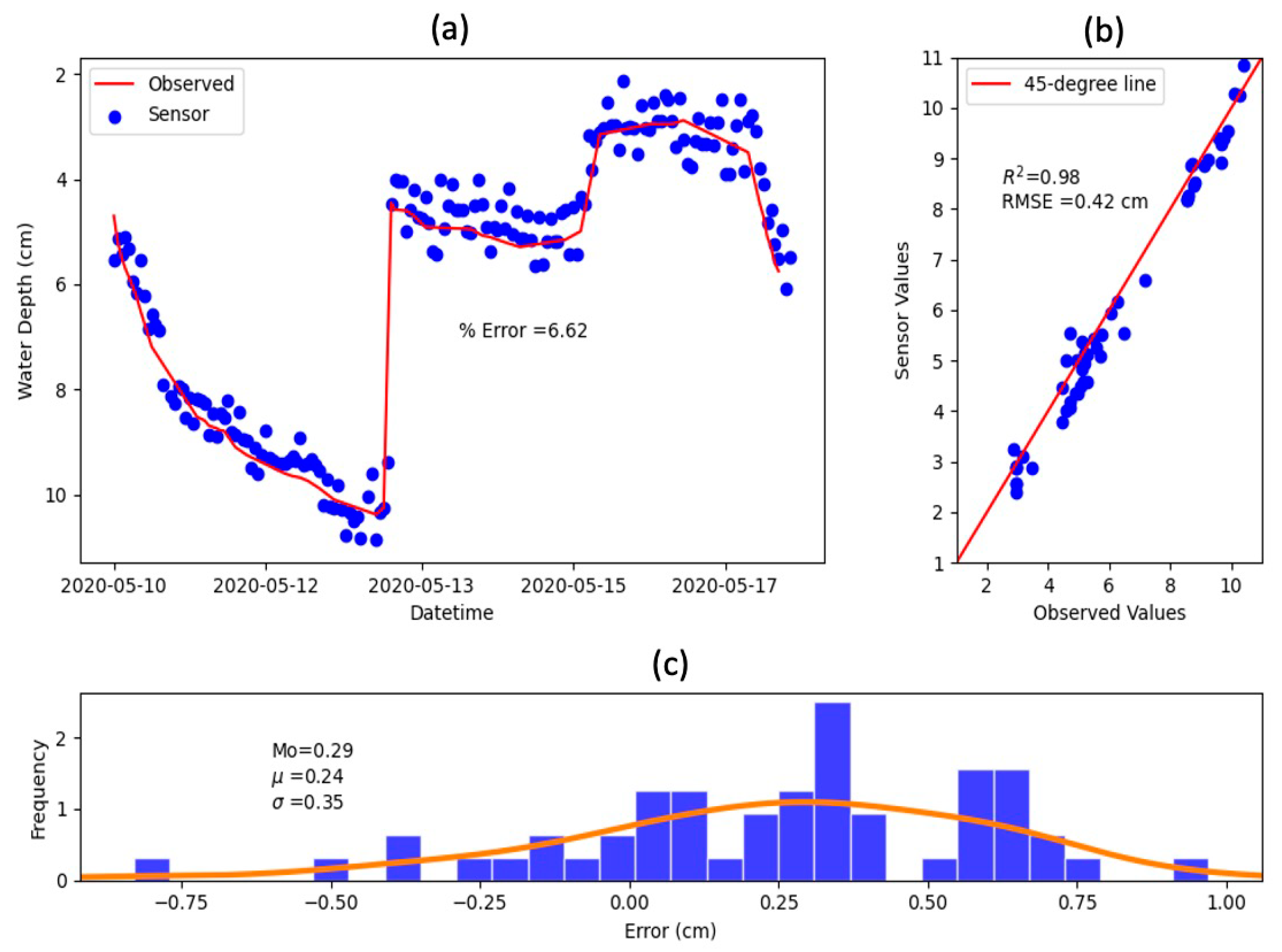
3.1. Laboratory Test Condition

Results from the laboratory tests are presented in Figure 7 and Figure 8. Sensor 1 exhibited error of 3.28% and RMSE of 0.46 cm, while sensor 2 had error of 6.62% and RMSE of 0.42 cm. Correlation between manual measurements and sensor measurements proved to be excellent for both sensors (R2 = 0.92 for Sensor 1 and R2 = 0.98 for Sensor 2). They also displayed the same degree of dispersion (σ = 0.35 cm), signifying that both demonstrate similar precision. However, the two sensors exhibited different tendencies when estimating the water level. Sensor 1 mostly overestimated the actual values with mode Mo = −0.28 cm and mean bias error 𝜇 = −0.29 cm, while Sensor 2 mostly underestimated the actual values with mode Mo = 0.29 cm and mean bias error 𝜇 = 0.24 cm. Even though the statistical parameters of both sensors were nearly identical in magnitude, both of their central tendencies were on the opposite side of the error distribution. A closer examination of the observed and sensor depth values from both test runs (Figure 7 and Figure 8) indicates that Sensor 2 measured relatively shallow depths, between 3 cm up to 10 cm, compared to Sensor 1 with water level ranges between 7 cm to 16 cm. It is important to note that the HC-SR04 ultrasonic water level sensor used in fabricating the low-cost sensor measures distances relative to where the sensor is located. Since the sensor is mounted at the top of the container, the reference elevation is the top of the container itself. Shorter sensor distance values mean deeper water levels in reference to the soil surface, while larger sensor distance values imply the opposite.
To further investigate the relationship of the errors with respect to water level depths, a simple linear regression was made (Figure 9). The R2 = −0.45 suggests that there exists a negative relationship between sensor accuracy and water level depths, albeit being moderate. But this moderate correlation influenced sensor readings in the millimeter range of accuracy. One investigator claimed these instabilities to be due to the lack of monotonicity, an occurrence of miscommunication between the components of the internal circuitry when reading peak signals [24]. Shorter ranges are more prone to these instabilities since the sensor processor tends to miss out faint peak signals from the comparator, resulting in longer duration before the echo pin signal goes low. This anomaly consequently results in longer travel time of sound, which further results to overestimation of measurements. However, the range of critical values was never established in the investigation. Having sufficient time for the sound waves to travel between the sensor and the target surface is highly advised in minimizing the occurrence of this anomaly. In this study, most of the overestimates were observed in ranges above 9 cm, while underestimates mostly occurred in even shorter ranges (less than 9 cm). Nevertheless, the sensor performance still remains to be acceptable from the economic viewpoint. The performance values of the low-cost sensor are also comparable to the water level sensor developed by Xiao et al. [21] and IRRI and PhilRice [19], which they claimed to be also suitable in paddy field conditions.

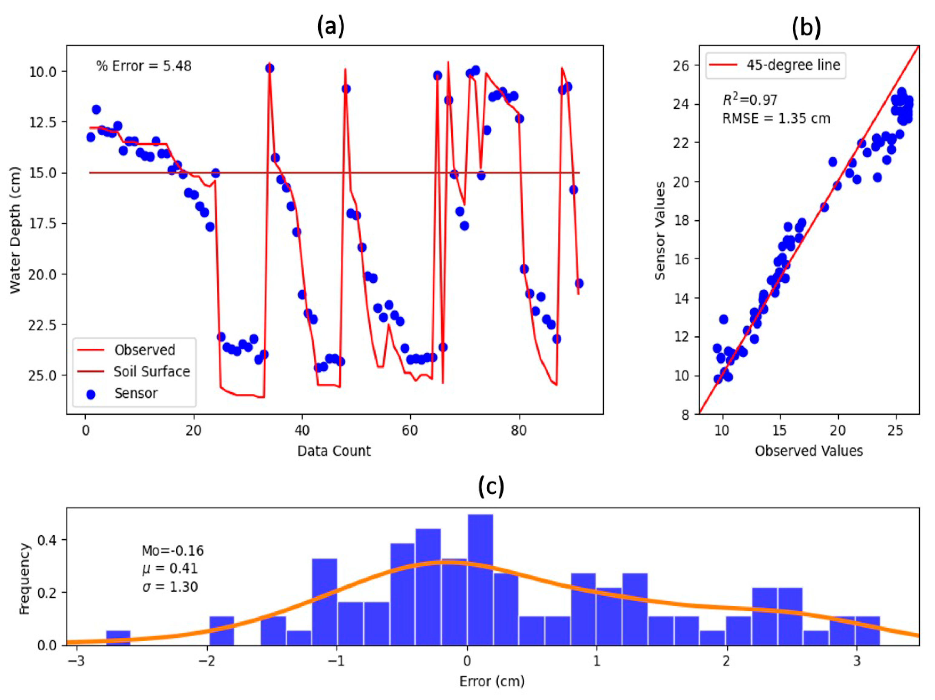
3.2. Pseudo-Field Test Condition

Results of the pseudo-field test runs are presented in Figure 10 and Figure 11. The performance of both Sensor 3 (5.48% Error and RMSE = 1.35 cm) and Sensor 4 (3.79% error and RMSE = 0.79 cm) proved to be reasonably acceptable with respect to manual measurements. Both sensors incurred a very high R2 above 0.97, suggesting an excellent correlation between sensor and manual measurements. The modes of both sensors in the error distribution (−0.16 cm and −0.03 cm for Sensor 3 and Sensor 4 respectively) imply that the sensors mostly estimate the water level at a high level of accuracy. Comparatively, the statistical performance indicators for Sensor 4 were better than for Sensor 3. The RMSE of Sensor 4 may be deemed acceptable from the practical standpoint. However, the performance of Sensor 3 greatly deviated from the initial sensor test under laboratory conditions (RMSE = 0.46 cm, σ = 0.35 cm and RMSE = 1.35 cm). This may largely be due to a relatively greater number of data points collected during low water levels, which comprised a fine portion of the dataset used to compare with the sensor values. Figure 10 shows an apparent pattern of consecutive underestimation of water level values at deeper levels, which is a complete disagreement from the observations in laboratory tests. While the internal circuit anomaly affects the sensor accuracy, the presence of successive underestimated values is indicative of an involved systematic factor. Albeit having Mo = −0.16 cm, the series of underestimated depths resulted in the dispersion of error on the positive side of the error distribution plot, consequently yielding a positive mean bias error of 0.41 cm. This occurrence may imply a possible problem posed by sediment accumulation at the bottom of the pipe in the actual field deployment, as had been observed during the implementation of the experiment in the micropaddy. The sediments may not affect the ultrasonic sensor readings at higher water levels [23], but the effect can manifest itself during low water level conditions. Unlike the automated pipe with a sensor on top, the free exposure of the manually observed pipe to the atmospheric conditions provide a faster rate of surface evaporation with direct sunlight and free air circulation, thereby reducing the residence time of shallow waters suspended with sediments at the bottom of the pipe. This occurrence was not highly emphasized under the laboratory conditions, since both the manual and automated measurements were observed on the same transparent container. The effect of sedimentation was only made evident by separating the manually observed and sensor-equipped pipes.
Other than sedimentation, pipe settling was also observed during the test run of Sensor 3. Depending on the degree of the soil cultivation done, the AWD pipe can also recede in the soil subsurface concurrently with the soil settlement as caused by the subsequent irrigation and drying cycles. The additional weight imposed by the sensor on top of the pipe may have also influenced the pipe recession, resulting to sensor measurement offsets from the manual observations.

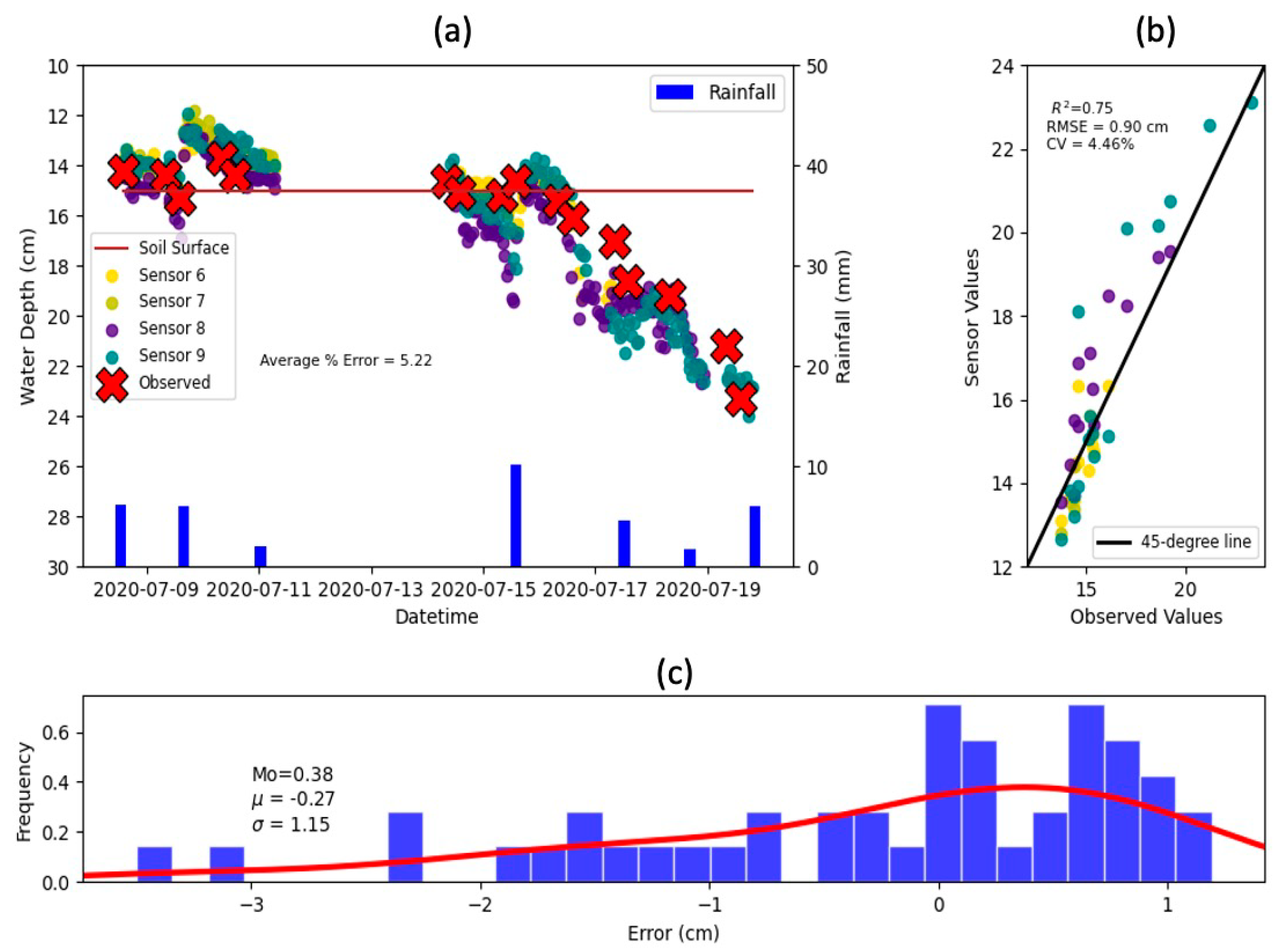
3.3. Actual Field Deployment

The results of the performance of the low-cost sensors installed under actual field conditions are presented in Figure 12. Sensor measurements exhibited a good correlation with manual measurements (R2 = 0.75) and showed an acceptable RMSE (0.90 cm). The average error (5.22%) also did not differ largely from the determined percentage errors in laboratory and pseudo-field conditions. The mode from the error distribution (Mo = 0.38) signifies that the sensors finely underestimated the actual depth in most cases, but the occasional overestimates were relatively large enough to draw the mean bias error (−0.27) into the negative side of the error distribution. The error dispersion (σ = 1.15 cm), however, may be the combined effect of many elements, including the tendency of the sensor itself to overestimate water levels at deeper depths, and the environmental factors in the actual field conditions. It may also be the reflection of slight water level variation in the field, considering the relative distances and placements of the sensors from one another. Moreover, a relatively low CV of 4.46% suggests that the data variation is highly acceptable. Using the same value of CV and assuming a 10% maximum allowable error, the optimum number of sensors N for the plot size considered becomes 0.20, which if rounded up to a practical value of N = 1 suggests that a single sensor is sufficient to monitor the field water level in the 14 × 44 m2 plot to generate at least 90% accuracy. It should be noted, however, that the optimum N may also vary with microtopographic variations and bund integrity among other factors, along with the desired accuracy of measurement. Further investigations are therefore recommended to establish the relationships between N and the aforementioned factors.
Aside from accurately representing the actual water level, the low-cost sensors were also able to provide a more defined pattern of water level fluctuations due to higher temporal resolution. This added information in between manual observation gaps can greatly facilitate the analysis of water balance dynamics in rice fields on an hourly basis, which is challenging to perform if the measurements are to be done manually. It can properly reflect water level fluctuations due to rainfall or irrigation, and water surface-subsurface recession due to water losses. Thus, the data generated by the low-cost sensor developed in this study can be used in the analysis of water fluxes and water balance in the field.

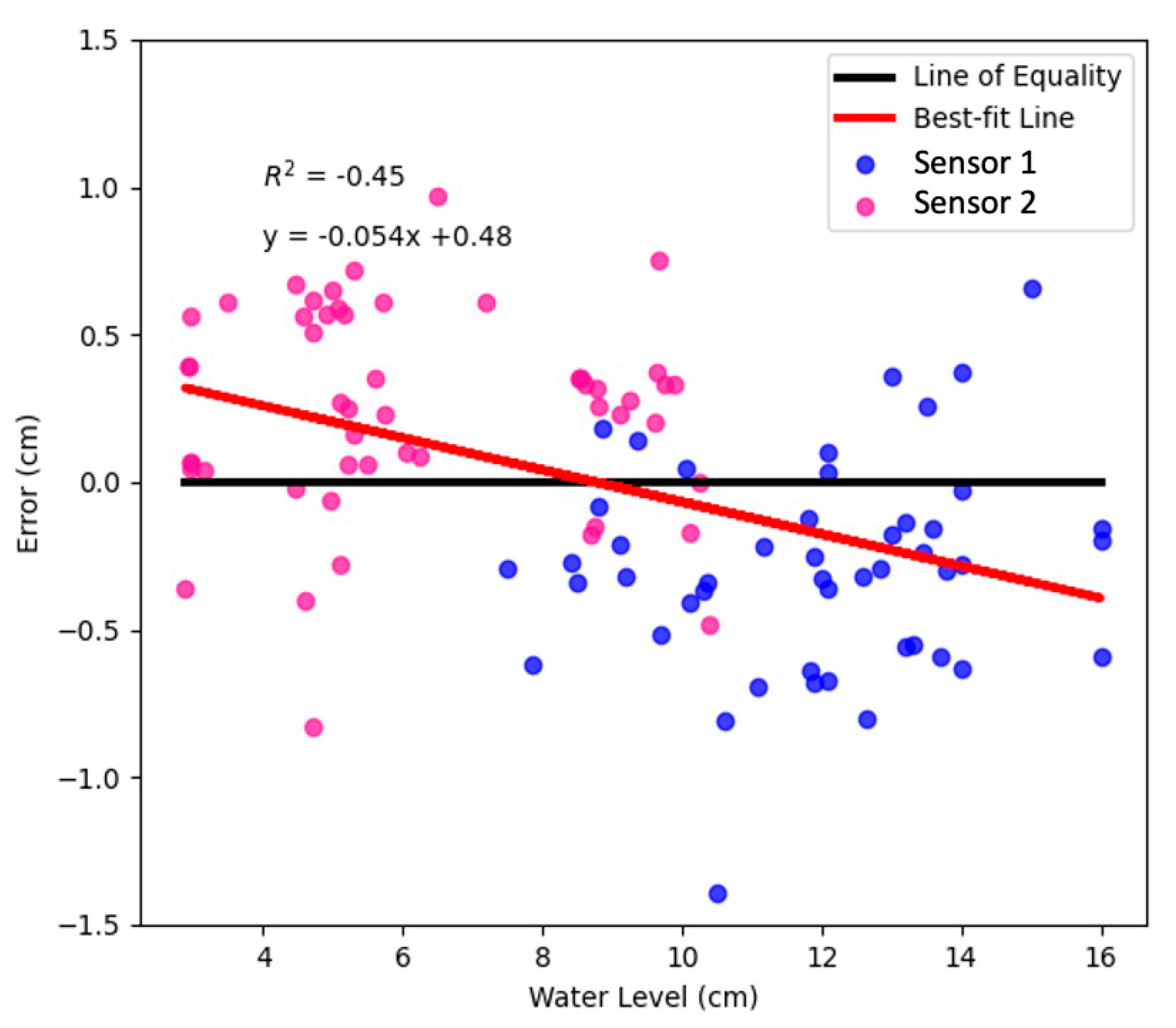
3.4. Performance Comparison between the Low-Cost Sensor and High-End Sensor

The performance comparison between the low-cost sensor developed in this study and a selected commercially available high-end sensor was performed in the micropaddy plot to facilitate measurements. Results are shown in Figure 13. Both sensors exhibited excellent correlation with the observed values (R2 = 0.96 for high-end and R2 = 0.98 for low-cost sensor) and relatively low RMSE (1.31 cm for high-end and 0.80 cm for low-cost sensor). Results further revealed that both the low-cost sensor and the high-end sensor mostly tend to reflect the actual water level, with Mo of 0.03 cm and 0.06 cm, respectively. Based on the previous sensor tests done, these modes are exceptionally accurate. However, the two sensors exhibited different error dispersion, with the high-end sensor (σ = 1.11 cm) showing wider spread than the low-cost (σ = 0.65 cm). The error dispersion of the high-end sensor resulted in less superior performance (%Error = 6.86; RMSE = 1.31 cm) than the low-cost (%Error = 5.16; RMSE = 0.80 cm). The high-end sensor’s data dispersion may be due to the extreme sensitivity of the sensor to pressure changes, particularly in higher water levels. The water turbidity may also have a direct influence on this sensitivity, although further investigations are necessary. On the other hand, there is still a tendency for the low-cost sensor to underestimate water level on shallow depths, with a local maximum of 1.10 cm. Nevertheless, Mo = 0.06 cm remains more dominant, suggesting a higher tendency for accurate readings. While further tests under actual field conditions may be necessary, the results from this test under pseudo-field conditions further prove that the performance of the low-cost wireless sensor developed in this study is practically at par with that of the high-end sensor.

3.5. Strengths and Limitations of the Developed Low-Cost Wireless Sensor

The use of noncontact-type sensors, such as the ultrasonic sensor of the low-cost, in measuring field water depths has the advantage in the paddy field setting. In contrast to the probe type sensors, the low-cost sensor is not prone to corrosion and hardware malfunction due to sedimentation problems. This was further supported by Chiu and Reba [15] in their findings. The low-cost sensor also makes use of less wires exposed outside of the sensor case, thus it is less likely to be damaged by field pests such as rodents. The sensor is also easy to use and maintain. The database system and alert messaging services can also be accessed free for as long as the Wi-Fi connection is available. Affordability is also one of the low-cost sensor’s most distinctive advantages over high-end sensors.
While the low-cost wireless sensor exhibits several advantages in terms of performance and costs, it still has a number of limitations. Firstly, the low-cost sensor does not have a real-time clock due to limited I/O pins; hence, the data encoded in the text file have no date and time stamps. However, manual data sorting can still be done by holding on to the logic of hourly sensor reading and comparing the data log entries in the text file with the online database entries. Secondly, the low-cost sensor is Wi-Fi-based, which makes the sensor range limited. Its application in rice field areas situated in off-grid communities would therefore pose a challenge. Obviously, the low-cost sensor, such as the high-end sensors, can only be effective in agricultural areas with a power source and Wi-Fi or at least signal extenders. Thirdly, the quality of Wi-Fi connection in the field may be affected by the rice canopy if the low-cost sensor is not placed strategically in the field. Fourthly, the low-cost sensor is not flood-proof, which makes it more viable to use during the dry cropping season. These identified limitations could serve as a basis for further research and development.

4. Conclusions

The low-cost wireless sensor developed and tested in this study can provide reliable information of paddy field water level in real-time to facilitate the application of AWD in rice production systems. Laboratory tests and analysis showed that the sensors developed can generate accurate readings. The pseudo-field test additionally revealed the influence of sedimentation and pipe settlement in sensor readings, causing measurement offsets from manual observations. When applied under actual field conditions, the low-cost sensor performed reasonably well from the practical standpoint, in spite of several environmental factors affecting the sensor accuracy. The performance of the low-cost sensor also proved to be comparable with that of the high-end sensor, exhibiting practically similar measurement accuracy and higher precision. Considering the low-cost sensor’s tested performance and economic edge, it can prove useful in the efficient irrigation water management in lowland rice crop production systems in developing countries, particularly during the dry season and under water-scarce conditions as a result of climate change and climate variability. Ultimately, the low-cost sensor can serve as a tool for climate change adaptation and mitigation strategies in lowland rice crop production systems through the AWD technology.

Author Contributions

K.M.S.D.C.: Conceptualization, methodology, investigation, formal analysis, visualization, writing—original draft, funding acquisition; V.B.E.: conceptualization, supervision, methodology, resources, project administration, funding acquisition, writing—review and editing; D.C.S.: supervision, writing—review and editing; G.S.P.: data curation; E.S.A.: data curation. All authors have read and agreed to the published version of the manuscript.

Funding

This study was supported by the Commission on Higher Education—Philippine-California Advanced Research Institutes (CHED-PCARI) through the PCARI WiSEIr project titled “Development of wireless sensor network-based water information system for efficient irrigation water management in the Philippines.” with project ID 2016-008. Additional funding was provided by the Philippine Council for Agriculture, Aquatic, and Natural Resources Research and Development (PCAARRD) of the Department of Science and Technology (DOST) through their MSc Thesis Financial Assistance Program.

Data Availability Statement

Datasets are available upon reasonable request.

Conflicts of Interest

The authors declare no conflict of interest.

Appendix A

Table A1. Sample dataset from the online database of the low-cost sensor during laboratory test conditions.
No.DateTimeWater Depth (cm)Temperature (°C)Humidity (%)Battey Voltage (Volts)
110-May-202010:26:31 AM5.5336.81493.76
210-May-202011:27:02 AM5.1441.19513.87
310-May-202012:27:13 PM5.4240.75693.92
410-May-20201:27:25 PM5.0940.94703.94
510-May-20202:27:24 PM5.3243.00643.92
610-May-20203:27:48 PM5.9541.81633.95
710-May-20204:27:35 PM6.1640.38603.96
810-May-20205:26:46 PM5.5335.00623.94
910-May-20206:25:32 PM6.2332.88673.93
1010-May-20207:25:01 PM6.8532.00743.93
1110-May-20208:24:43 PM6.5831.06723.93
1210-May-20209:24:30 PM6.7630.19713.93
1310-May-202010:24:26 PM6.8729.94703.93
1410-May-202011:24:11 PM7.9129.25693.93
1511-May-20201:23:27 AM8.1428.62693.93
1611-May-20202:23:12 AM8.2628.19693.93
1711-May-20203:23:06 AM7.9327.94693.92
1811-May-20204:23:00 AM7.9827.75693.92
1911-May-20205:23:01 AM8.5427.50693.92
2011-May-20206:23:05 AM8.1628.44693.92
2111-May-20207:23:38 AM8.6630.31693.92
2211-May-20208:24:28 AM8.1834.88683.94
2311-May-20209:25:46 AM8.2139.25734.01
2411-May-202010:26:27 AM8.2741.06784.05
2511-May-202011:26:36 AM8.8739.00784.09
2611-May-202012:26:41 PM8.4739.38754.11
2711-May-20201:27:02 PM8.8938.44754.1
2811-May-20202:27:20 PM8.4640.19734.13
2911-May-20203:27:53 PM8.5340.81654.14
3011-May-20204:27:38 PM8.238.44624.14
3111-May-20205:27:05 PM8.833.13604.13
3211-May-20206:26:00 PM8.8731.37684.13
3311-May-20207:25:24 PM8.4430.50714.13
3411-May-20208:25:19 PM8.9529.94704.13
3511-May-20209:25:01 PM8.9729.81704.13
3611-May-202010:24:57 PM9.5029.19694.12
3711-May-202011:24:55 PM9.1128.94694.13
3812-May-202012:24:44 AM9.628.56694.12
3912-May-20201:24:40 AM9.2428.31694.12
4012-May-20202:24:35 AM8.7928.25694.12
4112-May-20203:24:36 AM9.3128.25694.11
4212-May-20204:24:31 AM9.3628.00694.11
4312-May-20205:24:25 AM9.4127.44694.11
4412-May-20206:24:29 AM9.4028.19704.11
4512-May-20207:24:54 AM9.4030.06694.11
4612-May-20208:26:07 AM9.3633.50694.15
4712-May-20209:27:39 AM9.2839.50734.18
4812-May-202010:28:13 AM9.3638.94814.19
4912-May-202011:28:07 AM8.9339.75814.22
5012-May-202012:28:00 PM9.4340.19794.24
5112-May-20201:28:17 PM9.4138.13764.24
5212-May-20202:28:28 PM9.3441.13734.24
5312-May-20203:28:53 PM9.4342.00654.23
5412-May-20204:28:48 PM9.5536.25604.22
5512-May-20205:27:05 PM10.2033.50604.22
5612-May-20206:26:20 PM9.7231.75724.21
5712-May-20207:26:08 PM10.2331.44704.21
5812-May-20208:25:48 PM10.2729.94704.20
5912-May-20209:25:42 PM9.8129.63694.20
6012-May-202010:25:48 PM10.2829.37694.20

References

  1. Kumar, A.; Katagami, M. Developing and Disseminating Water-Saving Technologies in Asia; Asian Development Bank: Manila, Philippines, 2016; Policy Brief 60; Available online: https://www.adb.org/sites/default/files/publication/185485/water-saving-rice-tech.pdf (accessed on 1 April 2022).
  2. FAO. Emissions due to agriculture. In Global, Regional and Country Trends 2000–2018; FAOSTAT Analytical Briefs 18; Food and Agriculture Organization: Rome, Italy, 2020. [Google Scholar]
  3. GRiSP (Global Rice Partnership). Rice Almanac, 4th ed.; International Rice Research Institute: Los Baños, Philippines, 2013. [Google Scholar]
  4. Bouman, B.A.M.; Lampayan, R.M.; Tuong, T.P. Water Management in Irrigated Rice: Coping with Water Scarcity; International Rice Research Institute: Los Baños, Philippines, 2007. [Google Scholar]
  5. Lampayan, R.M.; Samoy-Pascual, K.C.; Sibayan, E.B.; Ella, V.B.; Jayag, O.P.; Cabangon, R.J.; Bouman, B.A.M. Effects of alternate wetting and drying (AWD) threshold level and plant seedling age on crop performance, water input, and water productivity of transplanted rice in Central Luzon, Philippines. Paddy Water Environ. 2014, 13, 215–227. [Google Scholar] [CrossRef]
  6. Carrijo, D.R.; Lundy, M.E.; Linquist, B.A. Rice yields and water use under alternate wetting and drying irrigation: A meta-analysis. Field Crop. Res. 2017, 203, 173–180. [Google Scholar] [CrossRef]
  7. Howell, K.R.; Shrestha, P.; Dodd, I.C. Alternate wetting and drying irrigation maintained rice yields despite half the irrigation volume, but is currently unlikely to be adopted by smallholder lowland rice farmers in Nepal. Food Energy Secur. 2015, 4, 144–157. [Google Scholar] [CrossRef] [PubMed] [Green Version]
  8. Linquist, B.A.; Anders, M.M.; Adviento-Borbe, M.A.A.; Chaney, R.L.; Nalley, L.L.; da Rosa, E.F.F.; Van Kessel, C. Reducing greenhouse gas emissions, water use, and grain arsenic levels in rice systems. Glob. Chang. Biol. 2015, 21, 407–417. [Google Scholar] [CrossRef] [PubMed]
  9. Lagomarsino, A.; Agnelli, A.E.; Linquist, B.; Adviento-Borbe, M.A.; Agnelli, A.; Gavina, G.; Ravaglia, S.; Ferrara, R.M. Alternate Wetting and Drying of Rice Reduced CH4 Emissions but Triggered N2O Peaks in a Clayey Soil of Central Italy. Pedosphere 2016, 26, 533–548. [Google Scholar] [CrossRef]
  10. Chidthaisong, A.; Cha-Un, N.; Rossopa, B.; Buddaboon, C.; Kunuthai, C.; Sriphirom, P.; Towprayoon, S.; Tokida, T.; Padre, A.T.; Minamikawa, K. Evaluating the effects of alternate wetting and drying (AWD) on methane and nitrous oxide emissions from a paddy field in Thailand. Soil Sci. Plant Nutr. 2017, 64, 31–38. [Google Scholar] [CrossRef] [Green Version]
  11. Setyanto, P.; Pramono, A.; Adriany, T.A.; Susilawati, H.L.; Tokida, T.; Agnes, T.; Padre, A.T.; Minamikawa, K. Alternate wetting and drying reduces methane emission from a rice paddy in Central Java, Indonesia without yield loss. Soil Sci. Plant Nutr. 2017, 64, 23–30. [Google Scholar] [CrossRef]
  12. Balaine, N.; Carrijo, D.R.; Adviento-Borbe, M.A.; Linquist, B. Greenhouse Gases from Irrigated Rice Systems under Varying Severity of Alternate-Wetting and Drying Irrigation. Soil Sci. Soc. Am. J. 2019, 83, 1533–1541. [Google Scholar] [CrossRef]
  13. Sander, B.; Schneider, P.; Romasanta, R.; Samoy-Pascual, K.; Sibayan, E.; Asis, C.; Wassmann, R. Potential of Alternate Wetting and Drying Irrigation Practices for the Mitigation of GHG Emissions from Rice Fields: Two Cases in Central Luzon (Philippines). Agriculture 2020, 10, 350. [Google Scholar] [CrossRef]
  14. Hossain, M.M.; Islam, M.R. Farmers’ Participatory Alternate Wetting and Drying Irrigation Method Reduces Greenhouse Gas Emission and Improves Water Productivity and Paddy Yield in Bangladesh. Water 2022, 14, 1056. [Google Scholar] [CrossRef]
  15. Rejesus, R.M.; Palis, F.G.; Rodriguez, D.G.P.; Lampayan, R.M.; Bouman, B.A. Impact of the alternate wetting and drying (AWD) water-saving irrigation technique: Evidence from rice producers in the Philippines. Food Policy 2011, 36, 280–288. [Google Scholar] [CrossRef]
  16. Chiu, Y.-L.J.; Reba, M.L. Development of a Wireless Sensor Network for Tracking Flood Irrigation Management in Production-Sized Rice Fields in the Mid-South. Appl. Eng. Agric. 2020, 36, 703–715. [Google Scholar] [CrossRef]
  17. Pfitscher, L.L.; Bernardon, D.P.; Ferreira, A.A.B.; Heckler, M.V.T.; Thome, B.A.; Montani, P.D.B.; Fagundes, D.R. An automated irrigation system for rice cropping with remote supervision. In Proceedings of the 2011 International Conference on Power Engineering, Energy and Electrical Drives, Spain, Malaga, 11–13 May 2011. [Google Scholar]
  18. Jacob, P.; Simon, S. Development and deployment of wireless sensor network in paddy fields of Kuttanad. Int. J. Eng. Innov. Technol. 2012, 2, 84–88. [Google Scholar]
  19. IRRI; PhilRice. AutoMonPH—An IoT Based Irrigation Advisory Service. In A Comprehensive Solution for Landscape-Scale Sustainable Water Management in Rice; Synthesis Report 1.0; International Rice Research Institute (IRRI): LosBaños, Philippine; Philippine Rice Research Institute (PhilRice): Ligao, Philippine, 2020. [Google Scholar]
  20. Chiaradia, E.A.; Facchi, A.; Masseroni, D.; Ferrari, D.; Bischetti, G.B.; Gharsallah, O.; De Maria, S.C.; Rienzner, M.; Naldi, E.; Romani, M.; et al. An integrated, multisensor system for the continuous monitoring of water dynamics in rice fields under different irrigation regimes. Environ. Monit. Assess. 2015, 187, 586. [Google Scholar] [CrossRef] [PubMed]
  21. Xiao, D.; Feng, J.; Wang, N.; Luo, X.; Hu, Y. Integrated soil moisture and water depth sensor for paddy fields. Comput. Electron. Agric. 2013, 98, 214–221. [Google Scholar] [CrossRef]
  22. Ramirez, R.C.; Agulto, E.S.; Glaser, S.D.; Zhang, Z.; Hermocilla, J.C.; Ella, V.B. DEvelopment of real-time wireless sensor network—based water information system for efficient irrigation of upland and lowland crop production systems. In Proceedings of the IOP Conference Series: Earth and Environmental Science, Online, 25–26 February 2022. [Google Scholar] [CrossRef]
  23. Kawakami, Y.; Furuta, T.; Nakagawa, H.; Kitamura, T.; Kurosawa, K.; Kogami, K.; Tajino, N.; Tanaka, M. Rice cultivation support system equipped with water-level sensor system. In Proceedings of the 5th IFAC Conference on Sensing, Control and Automation Technologies for Agriculture AGRICONTROL 2016, Seattle, WA, USA, 14–17 August 2016; Volume 49, pp. 143–148. [Google Scholar]
  24. Pilling, D. HCSR04. 2015. Available online: https://www.davidpilling.com/wiki/index.php/HomePage (accessed on 22 January 2022).
Figure 1. Wiring diagram of the low-cost wireless sensor modules with labeled electronic components.
Water 14 04128 g001
Figure 2. Low-cost sensor’s deployment setup and circuit assembly with labeled electronic components.
Water 14 04128 g002
Figure 3. Algorithm of the low-cost wireless sensor operation.
Water 14 04128 g003
Figure 4. Algorithm of the online data logging and alert messaging scheme of the web app developed using Google App Script.
Water 14 04128 g004
Figure 5. Dashboard of the online database showing real-time data of water level, surface temperature, and humidity, as well as the battery voltage of the low-cost sensor.
Water 14 04128 g005
Figure 6. Experimental setup of the sensor testing under (a) laboratory condition, (b) pseudo-field condition, and (c) actual field condition.
Water 14 04128 g006
Figure 7. Laboratory-based performance test of Sensor 1 showing (a) observed and sensor’s water level measurements through time, (b) comparison of observed and sensor values, and (c) error (observed-sensor) distribution with Gaussian KDF fit.
Water 14 04128 g007
Figure 8. Laboratory-based performance test of Sensor 2 showing (a) observed and sensor’s water level measurements through time, (b) comparison of observed and sensor values, and (c) error (observed-sensor) distribution with Gaussian KDF fit.
Water 14 04128 g008
Figure 9. Comparison of errors of Sensors 1 and 2 with water level depth under laboratory conditions.
Water 14 04128 g009
Figure 10. Pseudo-field-based performance test of Sensor 3 showing (a) observed and sensor’s water level measurements, (b) comparison of observed and sensor values, and (c) error (observed-sensor) distribution with Gaussian KDF fit.
Water 14 04128 g010
Figure 11. Pseudo-field-based performance test of Sensor 4 showing (a) observed and sensor’s water level measurements, (b) comparison of observed and sensor values, and (c) error (observed-sensor) distribution with Gaussian KDF fit.
Water 14 04128 g011
Figure 12. Performance of the low-cost sensors in actual paddy field conditions showing (a) observed and sensors’ field water level measurements, (b) comparison of observed and sensors’ values, and (c) error (observed-sensor) distribution with Gaussian KDF fit.
Water 14 04128 g012
Figure 13. Performance comparison of Sensor 10 (low-cost) and high-end sensor showing (a) observed and sensors’ water level measurements, (b) comparison of observed and sensors’ values, and (c) error (observed-sensor) distribution with Gaussian KDF fit.
Water 14 04128 g013
Publisher’s Note: MDPI stays neutral with regard to jurisdictional claims in published maps and institutional affiliations.

