Article

Three-Dimensional Turbulent Flow Characteristics Near the Leading Edge of a Longitudinal Structure in the Presence of an Inclined Channel Bank

Department of Civil and Environmental Engineering, Lehigh University, Bethlehem, PA 18015, USA
*
Author to whom correspondence should be addressed.
Water 2022, 14(21), 3524; https://doi.org/10.3390/w14213524
Submission received: 12 October 2022 / Revised: 1 November 2022 / Accepted: 1 November 2022 / Published: 3 November 2022
(This article belongs to the Special Issue Sediment Transport in Open Channel Flow)

Abstract

:
The present work investigates turbulent flow structures and behavior near the leading edge of a longitudinal flow obstruction in an open channel with an inclined bank. A volumetric particle image velocimetry (VPIV) was employed to collect velocity data. The results indicate that a relatively moderate channel bank angle ( θ = 28 ) does not prevent the formation of a junction vortex (JV) system. Indeed, it is found that the JV system develops over the channel bank and extends to the leading edge of the flow obstruction. It is demonstrated that the main factor that strengthens the primary junction vortex (JV1) at the tip of the protrusion is the pronounced downward flow. The probability density functions (pdfs) of the velocity fluctuations specify that the JV1 oscillates aperiodically between the so-called zero-flow and back flow modes. This explains the amplification of TKE at its core. It is shown that the velocity difference between the peaks of the pdf increases from over the channel bank towards the tip of the flow obstruction. The aperiodic behavior of the JV1 is confirmed via the proper orthogonal decomposition (POD) technique. Specifically, it is demonstrated that the leading POD modes, associated with the JV system, contain lower energy content compared to periodic flows. The time-averaged vertical vorticity field verifies the presence of a tornado like vortex structure near the upstream face of the retaining wall. Finally, the results suggest that the largest bed shear stress values in the mean flow are located near the tip of the protrusion.

1. Introduction

Flow past bank protrusions is of paramount importance in many river engineering applications. The most common type of such structures are bridge abutments, groynes, and spur dikes. These structure are built to minimize bank erosion or to enhance river habitats [1,2]. Local flow dynamics are modified in the presence of bank protrusions. In extreme cases, this leads to the formation of very complex, large-scale energetic coherent structures. When they are situated, or are advected, to near a channel bed the boundary shear stress and the pressure fluctuations are amplified. As a result, when the bed is erodible sediment particles are entrained. This ultimately causes development of a scour hole which can undermine the integrity of infrastructure components [3].
Previous experimental [4,5,6] and numerical [7,8] studies dealing with turbulent flows around bridge abutments and spur dikes, mounted on one of the vertical sidewalls of a channel, have identified highly turbulent 3D flows within their proxies that consist of turbulent structures over a wide range of scales. The dominant coherent flow structures and relevant features around the foregoing obstructions include: the junction vortex (JV) system and the recirculating flow near the upstream base of the protrusion, the separated shear layer that originates from the leading edge of the obstruction, and the wake flow past the protrusion. It is important to note that the JV system around flow obstructions attached to one side of a channel is typically referred to as a horseshoe vortex system in the literature. However, since the overall shape of the system of coherent vortices that develops around bridge abutments and spur dikes does not resemble that of a horseshoe, the authors advocate that it is more appropriate to use a more generic term, such as JV system. This terminology is adopted for the rest of this document. The JV system is relevant in many areas of hydrodynamics, hydraulics, and aerodynamics. The primary cause of JV system is the adverse pressure that is imposed by the upstream face of the obstruction which decelerates the incoming flow [8]. The adverse pressure gradient forces the incoming boundary layer to separate and create vortical structures that form the JV system. Typically, the junction vortices follow the junction line along the upstream face of the flow obstacle towards the leading edge of the protrusion and then stretch and bend in the direction of the main flow in the channel [7]. The main vortex of the JV system is characterized by large-scale low-frequency bimodal unsteadiness. This was first introduced by Devenport [9] who investigated the flow past a wall-mounted wing at a Reynolds number of 1.15 × 10 5 , based on the bulk velocity and the maximum thickness of the wing. They demonstrated that the increase of the turbulent kinetic energy (TKE) and pressure fluctuations within the JV system primarily occur as this system alternates quasi-periodically between two preferred states, namely backflow and zeroflow modes. It has been widely demonstrated that the shear stress is increased in the areas underneath the JV system (see for example [7]). This highlights the role of the JV system on the initiation and subsequent development of a scour hole on alluvial channel beds. However, the pronounced flow acceleration close to the leading edge of river bank protrusions, the downflow at the upstream face of the flow obstructions, and the vortices shed within the separated shear layer can also locally elevate bed shear stress and contribute to local scouring [10].
Understanding the intricate flow features associated with the scouring phenomena around bridge abutments, spur dikes, and groynes has been an important research topic in river engineering for over fifty years [11,12,13]. For instance, there have been several attempts in measuring the 3D flow fields around a spur dike using an Acoustic Doppler Velocimeter (ADV). Kuhnle et al. [14,15], for example, measured the flow velocities around a submerged, trapezoidal-shape spur dike over fixed flat and scoured beds using an ADV. They reported that strong lateral flows are the dominant cause of local scour. They also specified that the boundary shear stresses for the scoured bed case are higher than those of the flat bed condition. Additionally, Duan et al. [6] measured the 3D velocities, TKE, and Reynolds shear stresses around a nonsubmerged, rectangular spur dike using an ADV. Their results showed that the development of local scour coincides with the location of high shear stresses resulting from the junction vorticies. They also identified that the JV system, observed in front of the spur dike, interacts with the downstream recirculation zone. Recently, Rehman and Hong [16] examined the influence of lateral flow contraction on bed shear stress using an ADV. Specifically, they investigated the effects of local turbulence on the bed shear stress in terms of Reynolds stress and turbulent kinetic energy, and suggested an empirical correction factor for the calculation of bed shear stress using turbulent kinetic energy. The intermittent and highly complex 3D behavior of such flows, however, is difficult to capture with ADV measurements. The point-wise methodology employed during these measurements, constitutes a major shortcoming of this technology, limiting its ability to describe only time-averaged flow features over the spatial domain.
In the past decade, the use of particle image velocimetry (PIV) based techniques have gained popularity because they can overcome the ADV limitations. Launay et al. [17], for example, employed a planar PIV (PPIV) system, consisting of one camera, to study the effect of the obstacle elongation (length over width ratio) on the JV system. They reported that an increase of the obstacle elongation leads to a higher adverse pressure gradient in front of the obstacle. Consequently, this increases the longitudinal dimension of the JV system. Zhang et al. [18] investigated turbulent flow within the local scour hole around a single non-submerged spur dike using a PPIV. Their findings suggest that the final geometry of the scour hole is attributed to the combined effects of the JV system and the wake vortex. Recently, Heydari and Diplas [19] employed a steroscopic PIV (SPIV) system, consisting of two cameras, to examine the underlying turbulent flow characteristics near the leading edge of a longitudinal protrusion installed over a gravel bed. The measurement plane in that study was perpendicular to the main flow direction. The authors indicated the existence of a vortex near the tip of the flow obstacle and suggested that it represents a section of a JV system that originates from the channel bank and moves towards the leading edge of the obstruction. Both the PPIV and SPIV systems are capable of recording velocity data almost instantaneously and non-intrusively. However, the measurement domain in both cases is limited to a single plane. One possible solution to overcome this limitation is the use of a volumetric PIV (VPIV) system with three or more cameras, that can measure velocity vector field within a 3D region of the flow. Despite its advantages, the authors are not aware of the application of a VPIV method in any study dealing with turbulent flow around river-bank protrusions (e.g., bridge abutments and spur dikes).
Although an extensive number of studies have been devoted to the understanding of the flow physics around obstructions attached to vertical channel banks (e.g., bridge abutments), very limited research has been dedicated to the flow dynamics near the base of longitudinal flow obstructions in the presence of an inclined channel bank [20,21]. These longitudinal bank protrusions are commonly called retaining walls and are built to protect river-banks and bridge abutments from the threatening impact of major floods. There are several important geometrical differences between the retaining wall structure considered in this study and the typical longitudinal flow obstructions reported in the literature. The first and foremost, the inclined channel bank reduces the extend of flow obstruction with distance from the water surface. Secondly, the junction between the upstream face of the retaining wall and the channel boundary lies entirely on the channel bank and is inclined with respect to the horizontal plane, or channel bed (see Figure 1). Therefore, the present study investigates a case with different and more complicated geometry compared to typical junction flows considered in the literature. As such, it augments the category of junction flows and enhances the available findings on this subject. Furthermore, it is worth repeating that it is representative of a number of engineering applications, for which much needed information about the flow behavior is currently lacking.
The present study represents a significant extension of the previous work conducted by Heydari and Diplas [19]. The goal of this study is to provide further insights into the flow dynamics within a larger and 3D measurement domain before the commencement of scour (flat-bed), but near the threshold of bed material motion condition. This objective is archived by careful analysis of experimental data collected via a VPIV system. In addition to classical flow characteristics (e.g., velocity, vorticity and TKE fields), we also analyze the 3D velocity data using the proper orthogonal decomposition (POD) method to further elucidate the underlying features of the flow and thus expand upon prior studies that used the same method on 2D measurement domains (e.g., see [22]). To the best of our knowledge, this is the first time that the POD method is applied on 3D velocity data within a 3D measurement area near a longitudinal flow obstruction. Combining the observations and results of this study with those reported by Heydari and Diplas [19], we can get a more complete understanding of the flow dynamics in the vicinity of a longitudinal wall obstruction, which influence local scour and the integrity of this structure.
The next sections of this document are organized in the following way. First, the experimental setup and flow measurement instruments are described. Next, time-resolved, time-averaged, and POD results are shown, discussed and compared with the literature. Finally, a summary and conclusion section is provided.

2. Experimental Setup and Flow Diagnostics

2.1. Physical Setup

The experiments were conducted in a 15 m long, 1.2 m wide and 0.6 m deep water recirculating flume, located at the Imbt Hydraulic Laboratory of Lehigh University. A schematic of the flume and the experimental setup are illustrated in Figure 1a. The vertical sides of the flume were made of Plexiglas and the bed was covered with material in the gravel range, having a median size of 3.6 mm. The thickness of the gravel bed was set to 10 cm. A 1 m long longitudinal structure representing a retaining wall was attached to the bank 10.2 m downstream of the channel inlet. It was made of Plexiglas and painted black to minimize laser light reflection. The distance from the channel inlet to the retaining wall allowed the flow to attain a fully developed condition before the obstruction. This was confirmed via the measurements of the streamwise velocity profiles with an ADV. The channel bank angle ( θ ) was set to a relatively moderate slope of 28 . The resulting mean flow contraction was 18.2%. The same gravel particles that were used as bed material were used to build the channel bank. Finally, to prevent local erosion, a layer of gravel particles was glued on to a plastic net with 4 × 4 mm2 openings and then it was securely attached to the channel bank and bed near the leading edge of the retaining wall.
The experiments were conducted near the threshold of motion condition of the bed material. The pertinent flow parameters are summarized in Table 1:

2.2. Flow Diagnostics, Measurement Domain, and Data Analysis

The velocity information were obtained via a digital VPIV system. It consisted of three PowerViewTM 4MP-180 cameras, a dual pulsed Nd:YAG laser with a wavelength of 532 nm, an articulating laser arm to assist delivering the laser at the desired locations, two cylindrical lenses with a focal length of −25 mm and −50 mm to expand the laser light in longitudinal and lateral directions, respectively, and a synchronizer. A mounting frame was used to fix the cameras near the channel side-wall. The cameras were calibrated after the flume was filled with water with a back-lit target with 0.2032 mm holes on its surface that were regularly spaced at 5 mm apart both in the horizontal and vertical directions. The VPIV laser light was projected to the area of interest from the free-surface. A thin Plexiglas board was placed on the free water surface, barely touching it, to minimize the laser light reflection and optical problems (Figure 2). It was supported with an aluminum arm attached to the channel side-wall.
The measurement domain is illustrated in Figure 2. It extends from the region over the channel bank ( 0.36 × H behind the leading edge of the retaining wall) to that within the main channel flow ( 0.22 × H beyond the tip of the retaining wall) (Figure 2). The width of the measurement volumes over the channel bank during each individual data collection time period, was limited to ≈ 0.09 × H . The width of the measurement volumes were enforced by the intense reflection of the laser light from the gravel particles. Each measurement volume was created by chopping the laser light at the top of the Plexiglas board using two black bands. This approach enabled a continuous data collection without the need to stop the water recirculation in the flume. Therefore, it ensured that the approaching flow characteristics remained the same over the entire duration of the experiment. In total, four equally spaced measurement volumes were used to cover the region over the channel bank (labeled M_1 to M_4 in Figure 2). Beyond the tip of the retaining wall, however, the width of measurement volume was increased to 0.22 × H and only a single measurement volume was necessary for the purpose of this study (M_5 in Figure 2). The length (the dimension in the flow direction) of the five volumes across the measurement domain was on average ≈ 0.55 × H .
The VPIV images were obtained and processed using the Insight V3V 4G software developed by TSI Inc. The sampling rate and duration within each measurement volume were set to 50 Hz and 50 s, respectively. With this setting, about 2500 instantaneous velocity fields were obtained for each measurement volume for further analysis. Silver coated spherical particles, made of glass, with a mean diameter of d p = 80.5 μ m, nominal density of ρ p = 1200 kg m 3 , and Stokes number ( S t = ρ p d p 2 18 μ f t f , where μ f is the dynamic fluid viscosity, and t f = H U 0 is the incoming flow characteristic time-scale) of 0.0012 were employed to trace flow trajectories.
The following major steps were taken to obtain valid velocity vectors from the VPIV images. First, the minimum background light intensity was subtracted from every photograph in order to remove the background scattered light. This helps enhancing the quality of images. Next, the 2D particle locations were determined in each image via the particle identification method. It is important to note that one VPIV capture collects six separate images, one from each of the three cameras at times t and t + Δ t , where Δ t is the time interval between two consecutive images. Following the particle identification step, the 3D position of the particles were calculated from the matched triplets (each triplet corresponds to a single particle). Afterward, a robust particle tracking method, explained in [23], was implemented to obtain 3D velocity vectors of the individual particles. Finally, global range and universal median filters were applied to detect and remove invalid velocity vectors, and the missing vectors were estimated via interpolation.

3. Results

3.1. Velocity Field

Figure 3 provides an overall view of the flow velocity in the vicinity of the retaining wall structure. It demonestrates the dimensionless time-averaged streamwise (<u>*), lateral (<v>*), and vertical (<w>*) velocity fields, where < > stands for time averaging and the asterisk symbol denotes non-dimensionality, within a vertical plane parallel to the main flow direction at Y H = 0.05 , a horizontal plane at Z H = 0.06 , and a vertical plane parallel to the upstream face of the retaining wall at X H = 0.03 , respectively. Note that the non-dimensionalization of the velocity components is performed employing U 0 
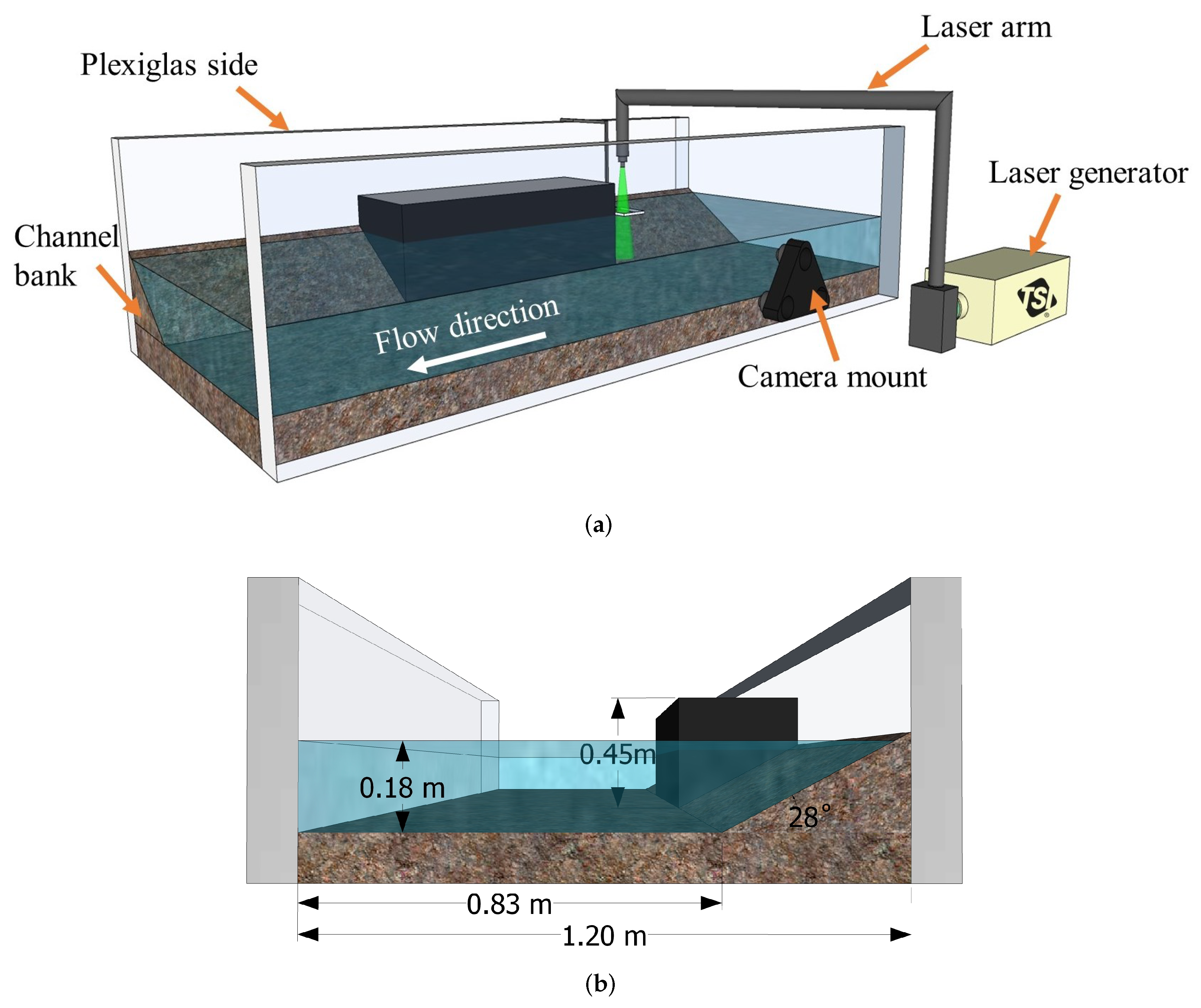
. Consistent with theory and observations reported by other researchers, the flow within the main channel accelerates near the tip of the retaining wall, which represents the location exhibiting the maximum local contraction of the flow [5,6]. This is clearly shown in the plane representing the streamwise velocity field (Figure 3). On the other hand, the flow decelerates as it approaches the upstream face of the longitudinal wall. The flow deceleration is the greatest near the free-surface, which, in turn, which results in the highest stagnation pressure. The stagnation pressure decreases towards the channel boundary in the vertical direction. As a consequence of this pressure gradient, a downflow is generated along the upstream face of the retaining wall, which acts like a vertical jet. Part of this flow penetrates into the channel bank, which acts like a porous boundary, and part of it is redirected in the transverse and upstream directions upon impingement on the channel bank boundary. The flow also experiences a strong lateral acceleration near the leading edge of the retaining wall because of a significant transverse pressure gradient that is due to the pronounced velocity difference between the flow over the channel bank and that within the main channel flow.
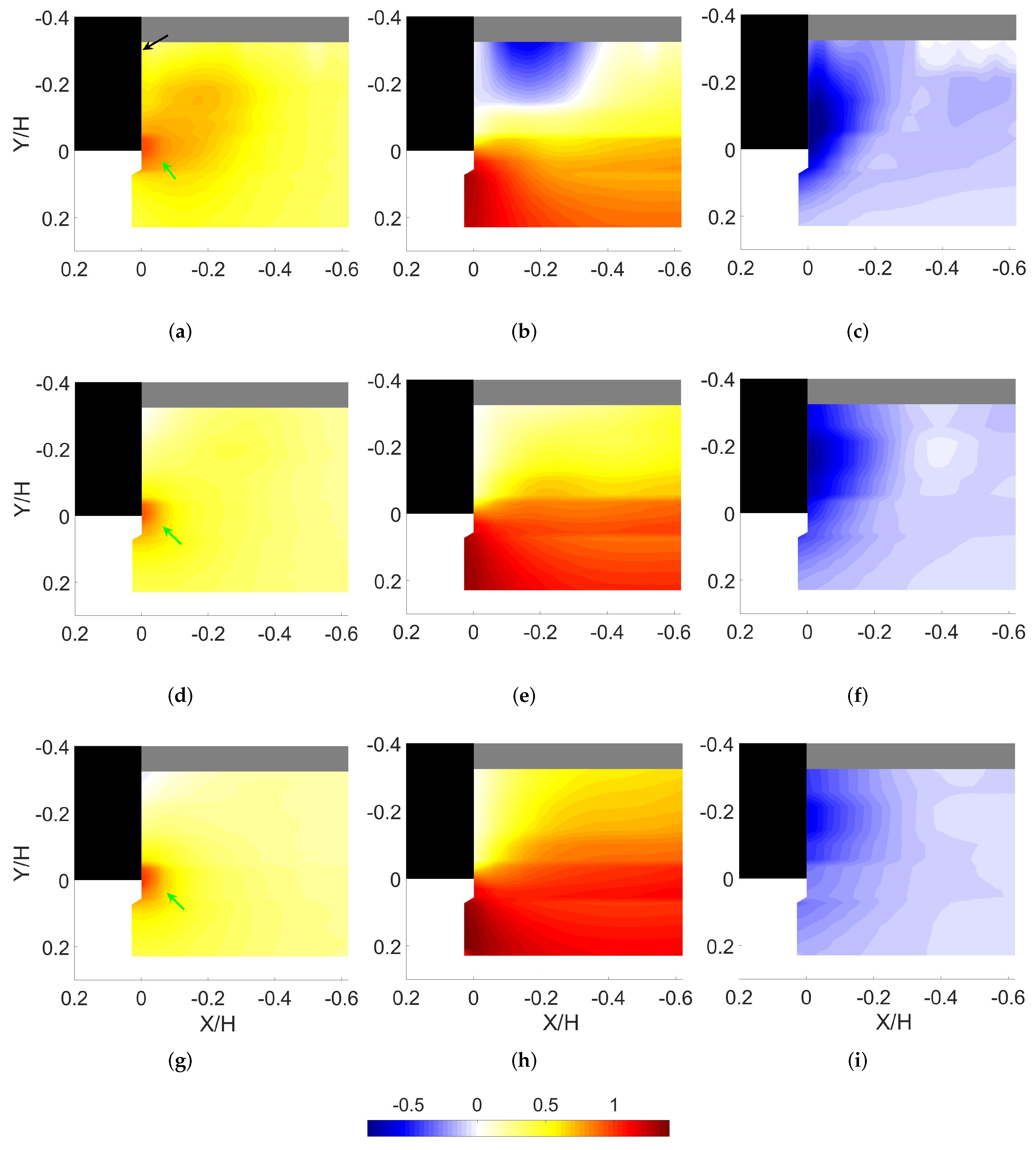
Figure 4 shows the distribution of the velocity components within horizontal planes located at different elevations from the channel bed (the black arrow in Figure 4a shows the upstream face of the flow obstruction). Specifically, Figure 4a–c show the velocity fields at Z H = 0.18 , Figure 4d–f correspond to Z H = 0.32 , and Figure 4g–i are related to Z H = 0.49 . The region of high lateral flow velocity, concentrated in the immediate vicinity of the leading edge of the protrusion, is indicated by a green arrow in Figure 4a,d,g. As shown in these figures, the lateral flow velocity near the upstream face of the flow obstruction is more pronounced near the channel bed (see the blob of high velocity region in Figure 4a). This is mainly attributed to the short distance between the leading edge of the retaining wall and the channel bank which the flow separates from because of the transverse pressure gradient. It is important to mention that due to the inclined channel bank, the degree of flow contraction decreases from its largest value at the free-surface to near zero at the channel bed. Therefore, most of the flow near the channel bed deflects laterally as it reaches the flow obstacle.
Figure 4b,e,h show the dimensionless time-averaged streamwise velocity fields at different elevations. A strong velocity gradient exists between the flow over the channel bank at the upstream face of the retaining wall and that within the main channel flow. This features a pronounced shear layer and is more evident in Figure 4b where there is a strong backflow region over the channel bank characterized by negative values of <u>*. The backflow contributes to the development of a JV system over the channel bank. The formation and characteristics of the JV system will be discussed in more detail in the next section. As the distance from the channel bed increases, the streamwise velocity component shows a more moderate variation from the regions over the channel bank to within the main channel flow (Figure 4h). Figure 4c,f,i illustrate the distribution of the vertical flow velocity component. As shown there, the downflow becomes more pronounced as one moves towards the flow obstruction. Specifically, the regions of high vertical flow velocity exist at X H > 0.27 . The downflow in front of the obstruction is advected towards the tip of the retaining wall by the JV system. Figure 3 and Figure 4 suggest that the downward velocity is not uniform (constant) over the upstream face of the retaining wall, instead it increases as the flow moves closer to the channel bank and then drops to near zero values at the solid boundary. This behavior is consistent with that in front of bridge piers, abutments, and spur dikes, where the vertical velocity changes almost parabolically from the free-surface to near the channel bed and assumes the maximum value slightly above the bed.
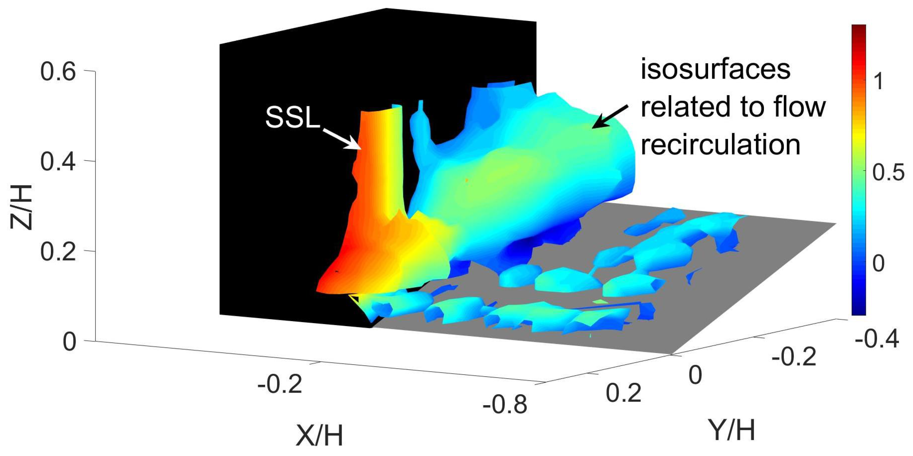
Figure 5 shows the dimensionless time-averaged vertical vorticity field (axis perpendicular to the channel bed in Z direction) within the VPIV measurement domain at different elevations from the channel bottom. The large absolute values of the vorticity in the vicinity of the leading edge of the flow obstruction are associated with the separated shear layer (SSL) that originates from the tip of the retaining wall. The isosurfaces of the dimensionless time-averaged vertical vorticity field that is plotted in Figure 6 clearly shows the SSL that extends to near the channel bed ( Z H = 0.09 ). Although no VPIV data are available beyond the leading edge of the retaining wall in the downstream direction, it is expected that, similar to the case of bridge abutments, small tube-like vortices form due to growth of Kelvin-Helmholtz instabilities. The size of these eddies grows in the downstream direction and, accordingly, their intensity decays with distance from the shedding region and finally they reattach to the longitudinal face of the retaining wall. The SSL locally induces intense bed shear stresses via high values of vertical vorticity (Figure 5a) and thus contributes to the overall development of local scour [24].
Another important observation in Figure 5 is the presence of a region of relatively strong vorticity near the upstream face of the retaining wall, indicated by a black arrow in Figure 5a–c. The isosurfaces corresponding to these structures are evident in Figure 6. This signifies the presence of a recirculation region over the channel bank. As one moves towards the free-surface, the blob of negative vorticity corresponding to the flow recirculation gets bigger in size, assumes smaller values, and moves towards the channel water margin. These characteristics explain why we can only observe part of the blob of the significant vorticity in Figure 5b,c. Examination of the TKE field within the corresponding horizontal planes (not shown here for the sake of brevity) indicated pronounced amplification of TKE within the aforementioned intense vorticity regions. These observations verify the previous hypothesis made by Heydari and Diplas [19] regarding the existence of a tornado like structure at the upstream face of the retaining wall similar to that around bridge abutments and spur dikes [7]. These eddies carry fluid and momentum from the free-surface towards the channel bed/bank [8]. The patches of positive vorticity in Figure 5a are related to the flow separation over the gravel particles resting on the channel bank. Their absence in Figure 5b,c is because of the distance of the edge of the measurement plane (over the channel bank) from the gravel particles resting on the channel bank.
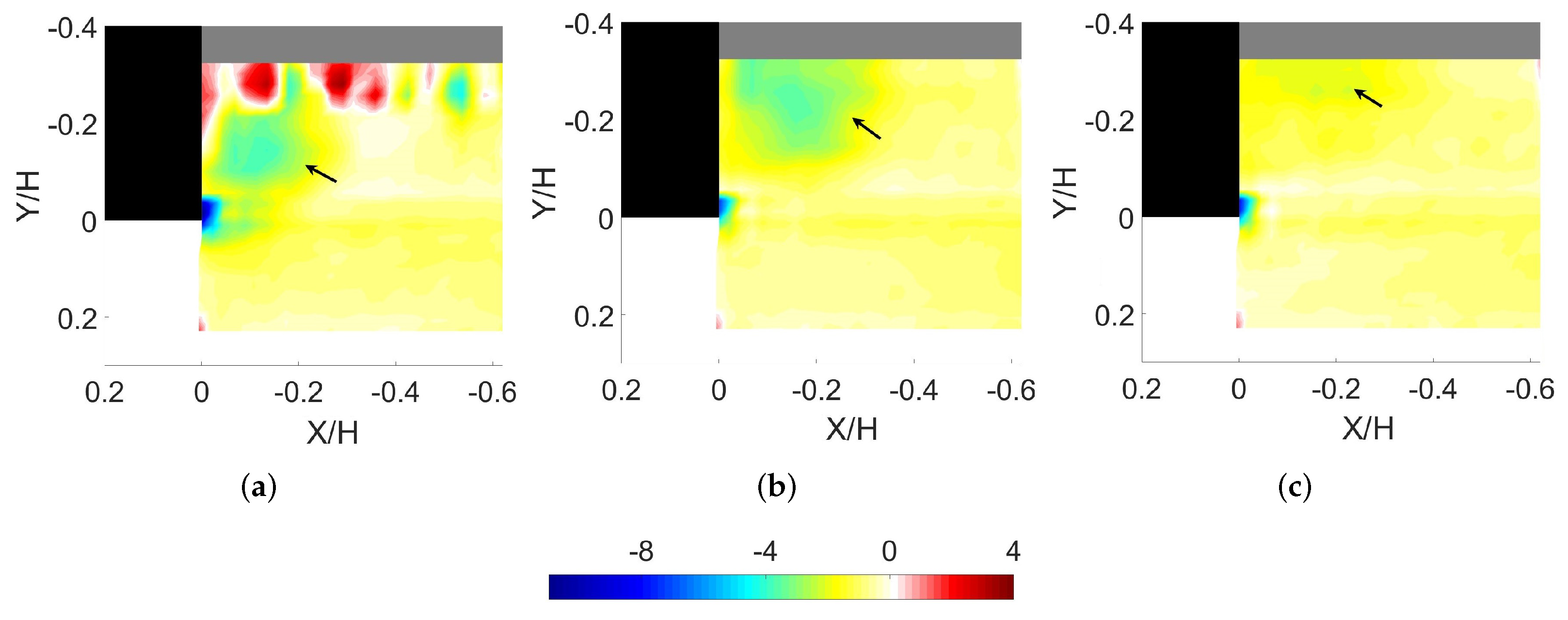
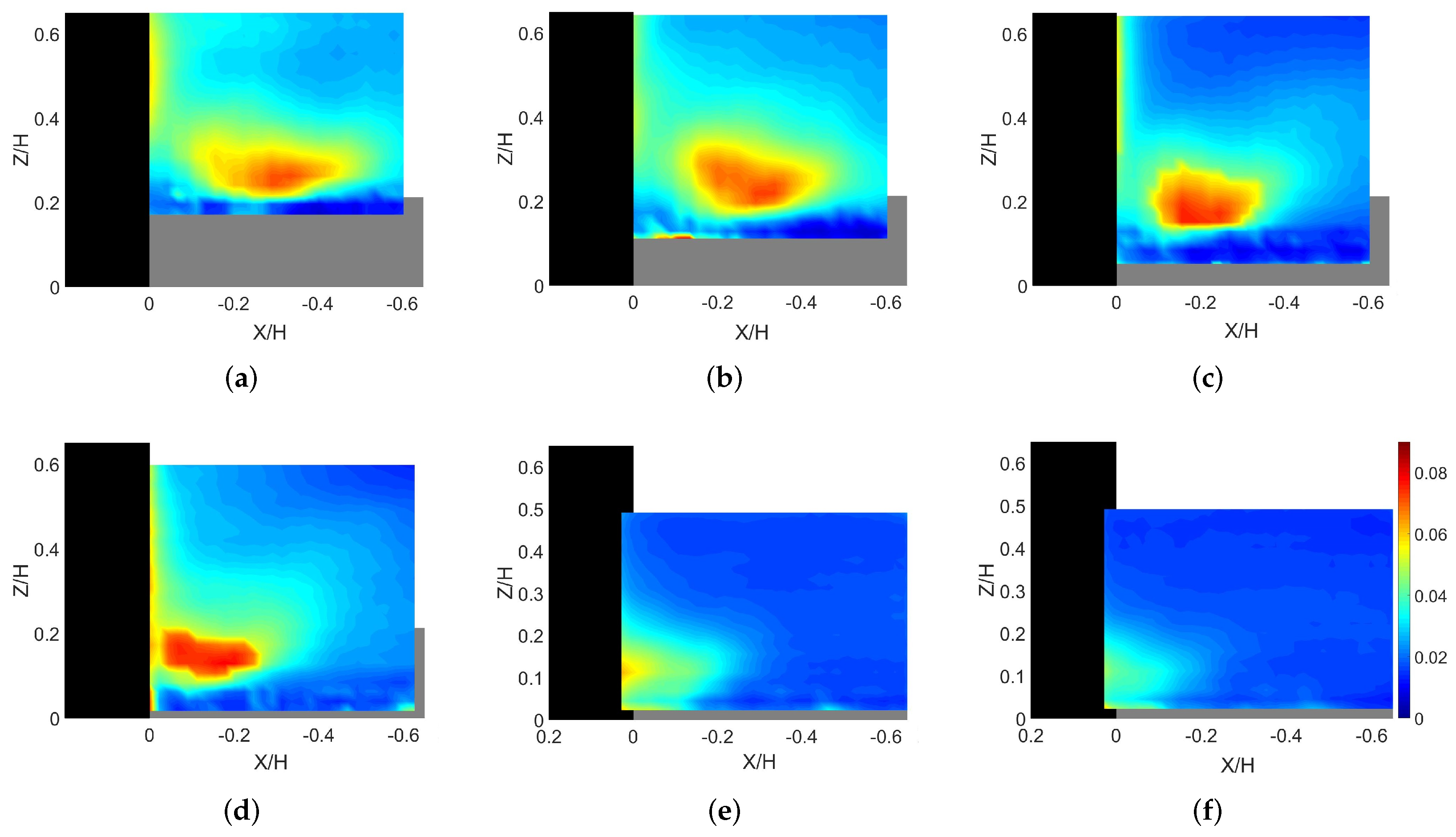
Figure 7a–c plot contour maps of the dimensionless < u v > component of kinematic Reynolds shear stress at Z H = 0.17 , 0.22, and 0.26 planes, respectively, where u and v are the velocity fluctuations in the streamwise and spanwise directions, respectively. Physically speaking, this term accounts for the momentum flux due to lateral turbulence mixing. In fact, it is related to < u > y . As illustrated in Figure 7, there exists a well-defined region with high values of < u v > whose location in each of the horizontal planes changes with distance from the channel bed. The shape and location of these regions, suggest that they are related to the presence of a tornado like structure at the upstream face of the retaining wall, as mentioned above. 
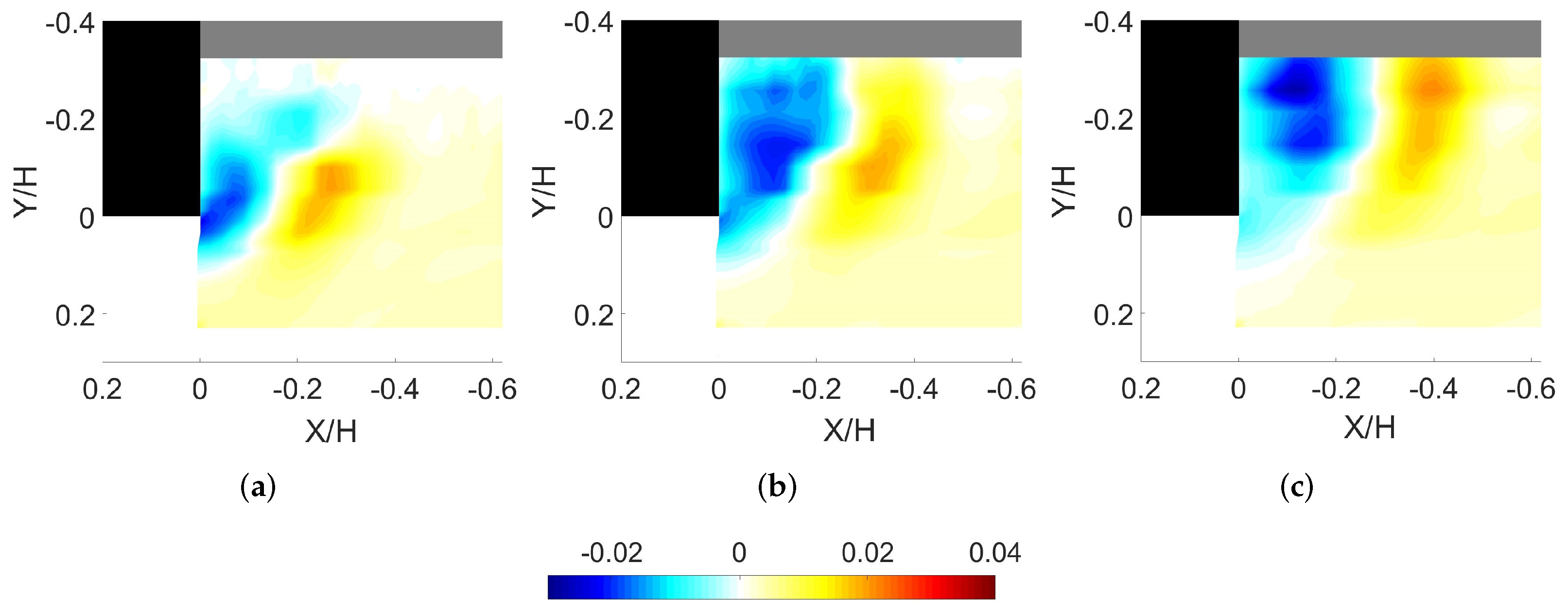
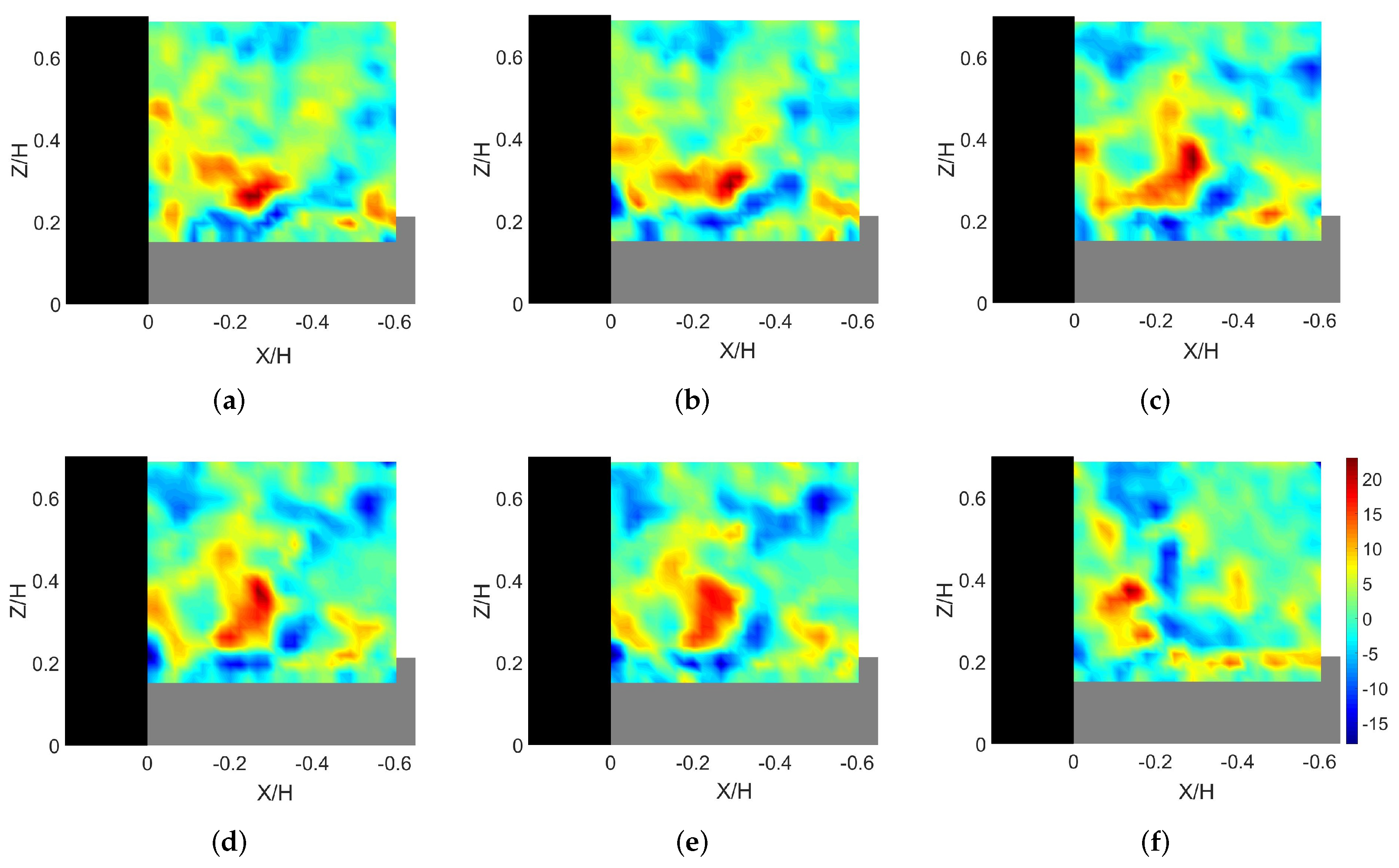
Figure 8a–c show the non-dimensional < u w > component of kinematic Reynolds shear stress, where w specifies the vertical flow velocity fluctuations. It denotes the vertical advection of streamwise turbulent momentum, or simply the turbulent shear stress caused by the streamwise velocity gradient in the vertical direction. One can notice that the areas near the leading edge of the retaining wall and close to the channel bed (Figure 8a) and the regions in the vicinity of the upstream face of the flow obstruction at higher elevations from the channel bed (over the channel bank) (Figure 8b,c) are dominated by negative values of < u w > stresses. This means that the streamwise velocity in these areas tends to decrease vertically (Z direction). Indeed, this is the case because of the near wall jet underneath the JV system that is generated via the downflow which upon impingement on the channel bank moves in the upstream direction. The negative regions of < u w > are accompanied by adjacent areas having positive values of < u w >. The positive stresses are consistent with the fact that the streamwise velocity in those locations, designated by yellow color in Figure 8, increases with the vertical distance from the bottom boundary.

3.2. JV System

JV system is an important hydrodynamic feature which directly influences the depth of local scour around flow obstructions. A detailed understanding of the JV system is, therefore, essential to reveal the underlying physics of scour around hydraulic structures. Consistent with previous research studies dealing with junction flows [5,
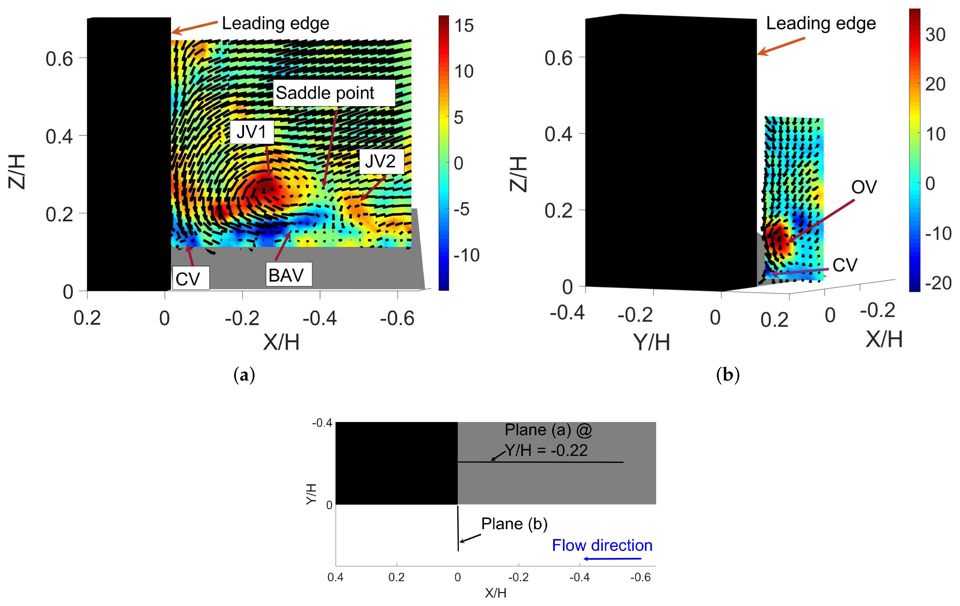
10], the investigation of the instantaneous velocity fields considered here indicated that as the flow approaches the protrusion it undergoes a very complex separation (highly 3D) over the channel bank because of the adverse pressure gradient (Figure 9a). Besides, as we showed in the previous section, there exists a strong downward flow at the upstream face of the retaining wall. These together generate a rotational motion, that has a counter-clockwise sense, near the slopping junction line created by the channel bank and the upstream face of the retaining wall, as shown in Figure 9a. The foregoing large-scale rotational motion is a section of a JV vortex system called primary JV (JV1). Due to the strong three-dimensionality of the flow, it is not easy to accurately specify the shape, position, and size of the flow structures based on the velocity vectors. Therefore, quantitative measures are more reliable. In this sense, the non-dimensional instantaneous vorticity field in the spanwise (Y) direction, ω Y * = ( u Z w X ) × H U 0 , is calculated and depicted in Figure 9a. There is a relatively weak and highly intermittent rotational motion upstream of the JV1. It has a smaller core size compared with the JV1, but it rotates in the same direction. This is referred to as a secondary junction vortex (JV2). These two rotational motions, JV1 and JV2, are separated by a saddle point. There are also patches of strong clockwise vorticity, called bottom attached vortices (BAV), that are ejected away from the channel bank. Their presence is an indication of a strong interaction between the JV1 and the channel bottom boundary. Indeed, a close examination of the instantaneous vorticity fields indicates that there are instants when the BAV disintegrate the JV1 from upstream and vorticity cancellation occurs. As a result the intensity and coherency of the JV1 decays for a certain period of time (see the next section for details). This observation is in agreement with the results from topological models inferred through flow visualizations [25,26]. The foregoing observations indicate that the presence of a channel bank with a mild angle ( θ 28 ), and the resulting inclined junction line, does not prevent the formation of a JV system, a typical feature of junction flows.
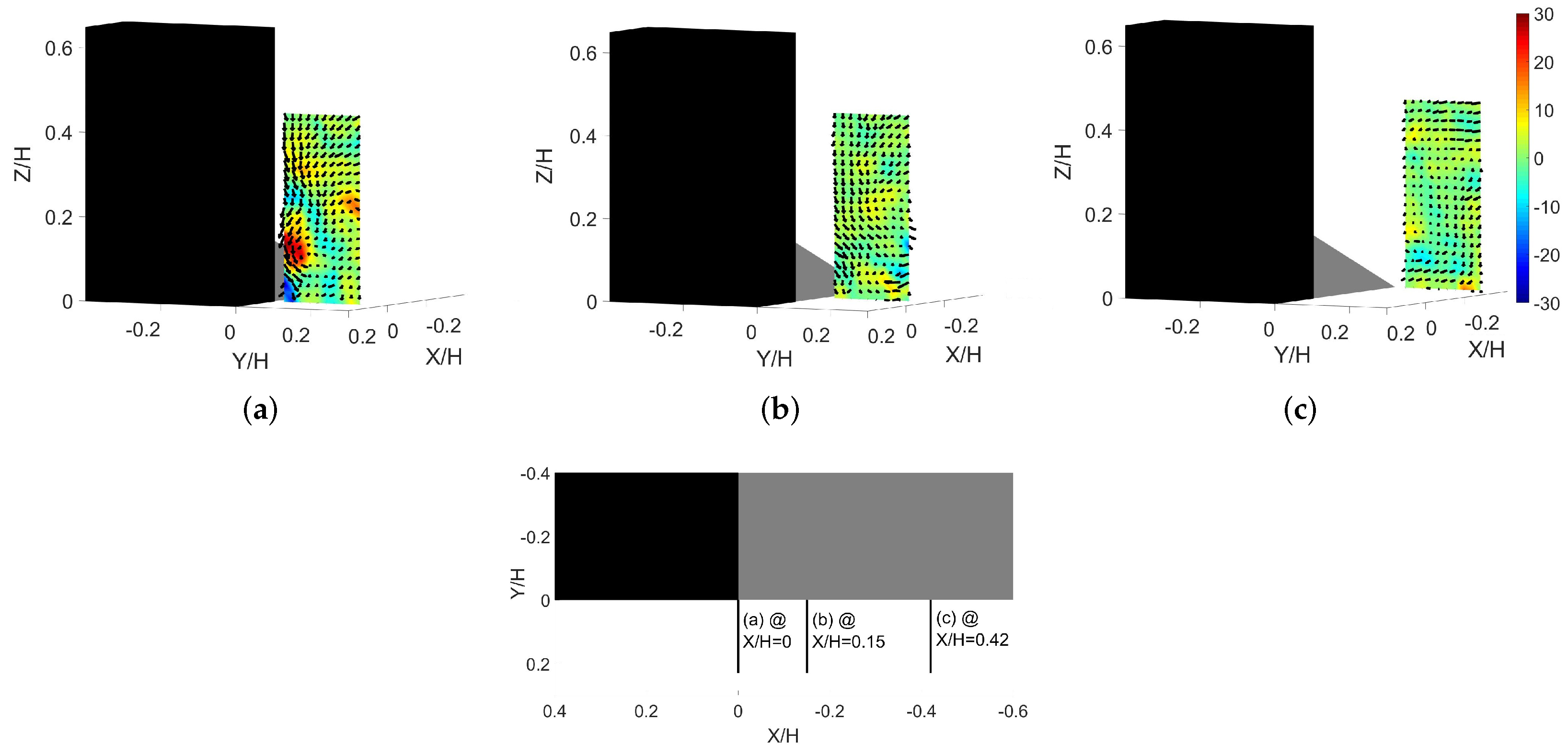
Another notable point is the presence of coherent structures in the vicinity of the retaining wall within the planes that are perpendicular to the mean flow direction (see for example Figure 9b, the background in this figure shows the ω X * ). The examination of the velocity snapshots indicate that these coherent motions are generated as a result of a strong downward flow which upon impingement on the channel bed wraps into the large-scale coherent structures, similar to those shown in the Figure 9b. These motions are called outer vortices and they are part of the JV system which develops near the upstream face of the retaining wall over the channel bank. The colorbars in Figure 9 imply that the magnitude of vorticity inside the outer vortex (OV) is larger than that inside the JV1 over the channel bank. A corner vortex (CV) is observed near the corner region created by the junction of leading edge of the retaining wall and the channel bed (Figure 9b), and also over the channel bank (Figure 9a). The formation of such vortices is related to the separation of fluid from the retaining wall’s face due to the adverse pressure gradient that is applied by the bottom boundary (channel bank/bed in our case).
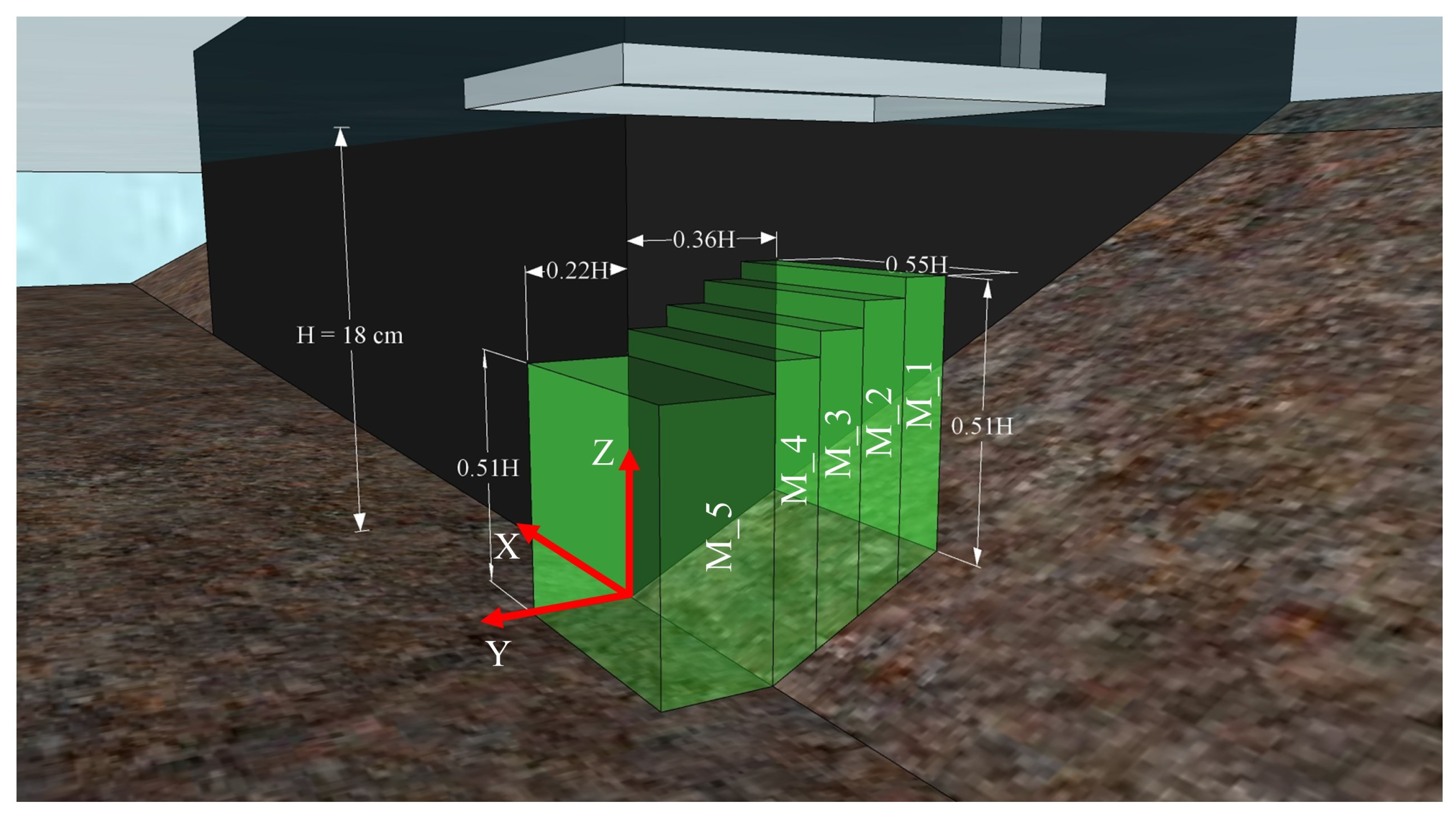
Before characterizing the JV system present in the mean flow, it is deemed appropriate to examine the instantaneous flow fields across the measurement domain. As described earlier in Section 2.2, the flow measurements were obtained in five discreet measurement volumes. Therefore, it is not possible to discuss the flow structure at a "particular" instant of time over the entire measurement region. However, the authors reached exactly the same results and conclusions after examining the flow field within each of the measurement volumes across the entire region under investigation over the duration of the experiment. 
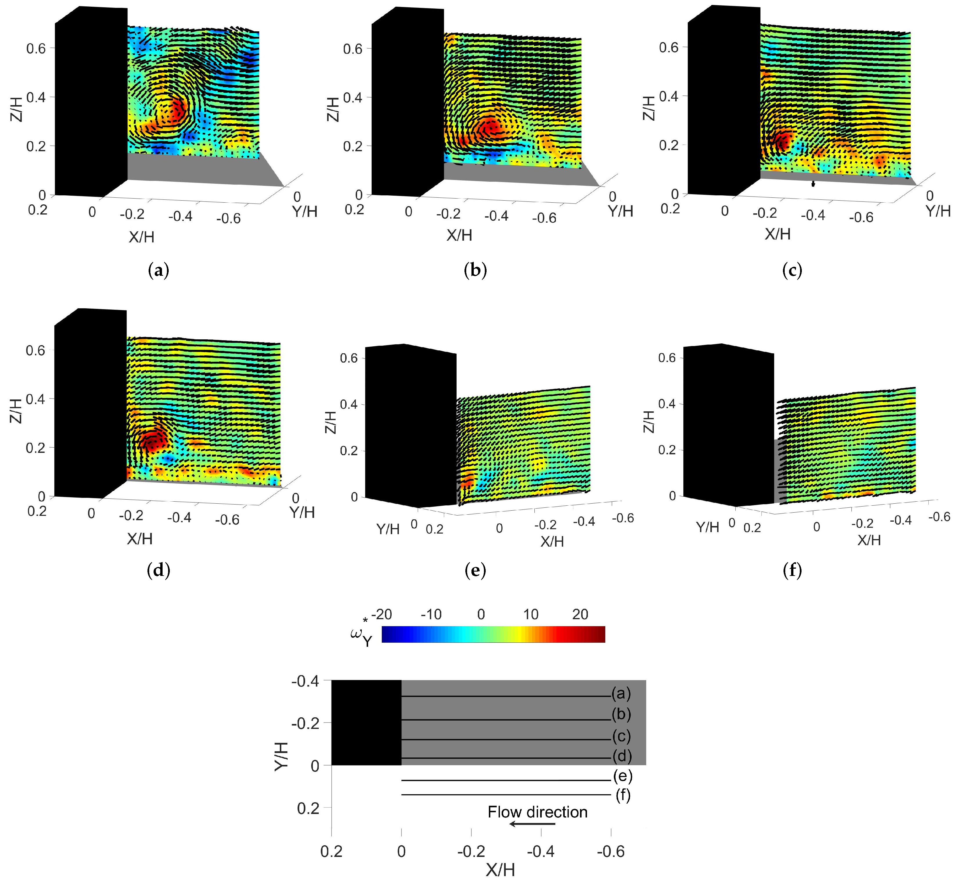
Figure 10 illustrates an oblique view of the instantaneous 3D velocity vectors and the contours of ω Y * within several representative planes over the channel bank and beyond the retaining wall within the main channel flow. The exact position of the measurement planes is determined in the plan view included in Figure 10. It is important to note that a different viewing angle was used in Figure 10e,f for better visual access purposes. Each of the flow fields corresponds to the same time instant (t = 38.34 s from the beginning of data collection period). A large vortex that corresponds to the JV1 is evident in all the frames over the channel bank (Figure 10a–d). However, as vorticity contours suggest, the structure of the JV1 is significantly dependent on its position. In particular, JV1 becomes more compact and relatively circular, while at the same time the intensity of vorticity at its core increases, as the flow moves towards the leading edge of the retaining wall. The magnitude of the ω Y * within the JV1 peaks near the tip of the retaining wall. As one would expect, beyond the leading edge of the retaining wall there is no adverse pressure gradient and thus the intensity of the JV system, JV1 in particular, decreases until it completely disappears. This aspect is shown in Figure 10e,f.
Another interesting observation from the instantaneous flow field shown in Figure 10 is that there is no obvious coherent structure associated with JV2 that persists across the measurement domain. This is because JV2 is, in general, smaller in size and lower in intensity than JV1, intermittent in nature, and not stationary in space. Examination of the video animations of the instantaneous velocity field in several planes over the channel bank indicated that JV2 moves off the plane of observation at several instants or it amalgamates with the JV1. Furthermore, it is important to note that the presence of the inclined channel bank reduces the level of obstruction to the approach flow and consequently the magnitude of the adverse pressure gradient against the incoming flow decreases. This, in turn, reduces the coherency and strength of the weak JV2 (an order of magnitude weaker compared to JV1). These features, along with the unsteady and three-dimensional nature of the flow make it difficult to distinguish and follow the JV2 within the measurement domain. Similar characteristics to those reported here have been documented for the JV2 near the upstream face of bridge abutments with sloped sidewalls [27], and upright wall mounted cylinders [28].
Figure 11 shows the instantaneous non-dimensional velocity vectors that are superimposed on the dimensionless streamwise vorticity field ( ω X * = ( w Y v Z ) × H U 0 ) in three representative measurement planes perpendicular to the main flow direction at a certain time instant. As shown there, the OV is more coherent and assumes larger values of vorticity within its core in the immediate vicinity of the leading edge of the retaining wall. As one moves in the upstream direction the coherency of the OV diminishes and, accordingly, the intensity of vorticity at its core decreases. This is primarily due to the downflow, the main source of the generation of the OV, which is more pronounced near the leading edge of retaining wall.
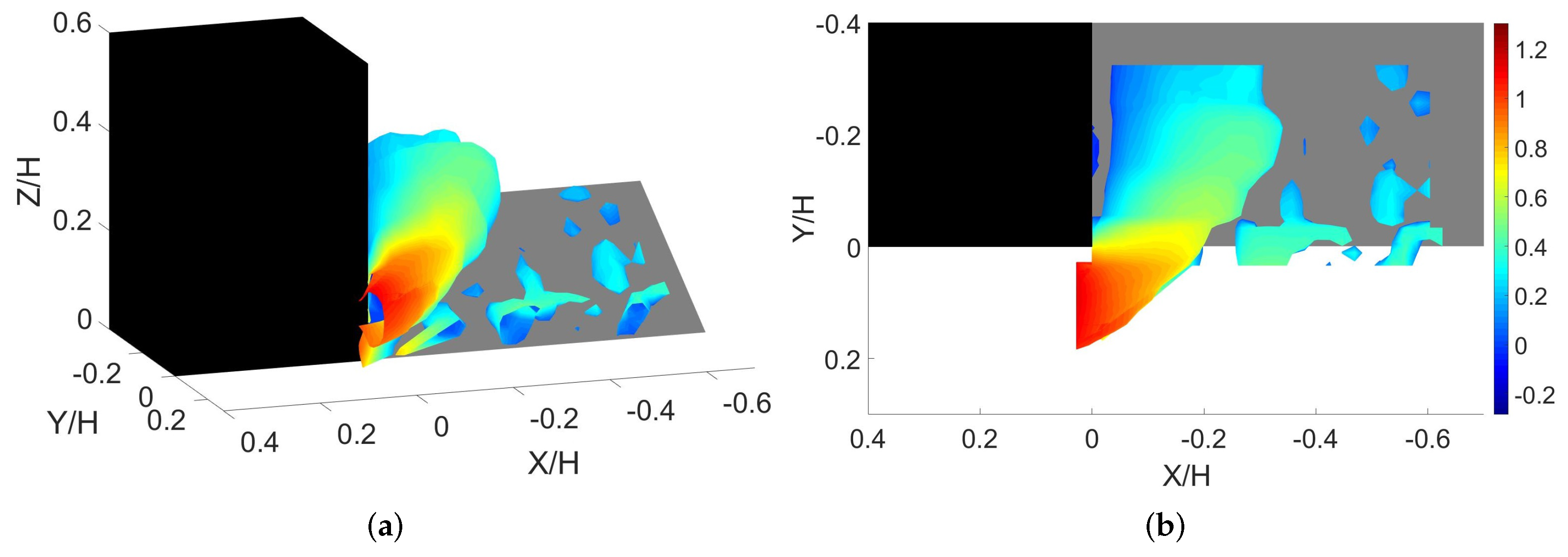
Figure 12 visualizes the JV system present in the mean flow using the Q-criterion (= 0.5 × ( Ω 2 S 2 ) , where Ω and S are the rotation and strain rates, respectively) [29]. The quantity Q is dimensionalized with ( H U 0 ) 2 and the corresponding isosurfaces at the isovalue of 2 are shown in Figure 12 (a 3D and a plan views are included there). The color coding corresponds to the dimensionless time-averaged streamwise velocity. The results show that JV1, which develops over the channel bank, with an almost elliptical cross-sectional shape, moves towards the tip of the retaining wall and gradually changes its direction from being almost parallel to the upstream face of the obstruction to eventually becoming nearly parallel to the main flow direction immediately past the leading edge of the retaining wall, where it assumes a circular shape. These observations confirm that the OV vortex is part of the JV system, JV1 in particular. Consistent with the instantaneous results, Figure 12 implies that the size of JV1 decreases towards the toe of the channel bank where the vorticity at its core, as illustrated in Figure 10, and its streamwise velocity attain peak values. It is therefore expected that the JV system exerts high bed shear stress in that area. Indeed, the authors confirmed that, via preliminary experiments over an erodible bed, local scour initiates right at the leading edge of the retaining wall, where ultimately the maximum scour depth was recorded as well. There observations were consistent for both fixed and erodible channel banks. More details about the characteristics of the maximum local scour depth at the base of retaining walls can be found in [20,21]. Finally, one can notice that there is no clear footprint of the JV2 in Figure 12. This confirms the weak and intermittent nature of JV2 that was discussed earlier in this section.
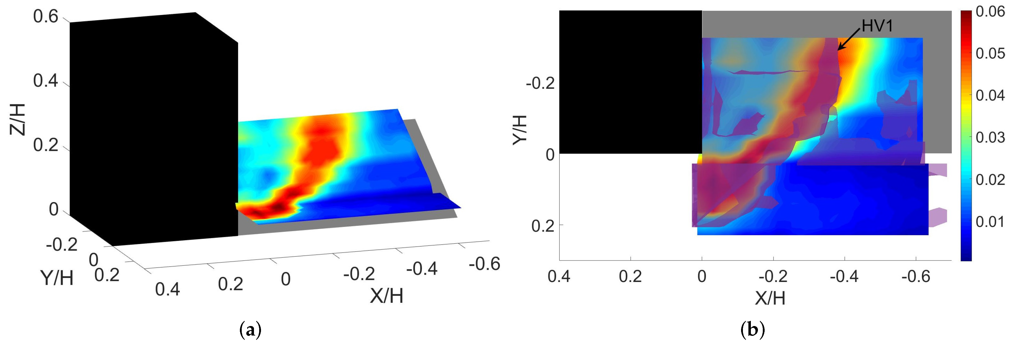
The distribution of the mean Reynolds shear stress near the channel bed and the channel bank, estimated as τ b * = τ x 2 + τ y 2 + τ z 2 U 0 2 , where τ x = ( < v u > + < w u > ) , τ y = ( < u v > + < w v > ) and τ z = ( < u w > + < v w > ) , is plotted in Figure 13. As shown in Figure 13a, the high τ b * values occur around the tip of the retaining wall, which coincides with the location of the local flow acceleration in that region. This is consistent with experimental observations of Rajaratnam and Nwachukwu [30] and Molinas et al. [13]. Figure 13b provides a top view of the isosurfaces of the JV1 over the plane showing the mean shear stress values. Note that a slightly lower isovalue, 1.5, is used here compared to the value of 2 used in Figure 12, to better illustrate the perimeter of JV1. As shown in Figure 13b, a relatively narrow band with significant values of shear stress, from over the channel bank to near the leading edge of the protrusion, nearly coincides with the path of JV1. Evidently, the high values of τ b * over the channel bank occur near the upstream end of the JV1, but towards the tip of the retaining wall they take place right beneath the core of JV1. Therefore, one can conclude that the increase of shear stress beneath JV1 at the tip of the retaining wall is due to the combined action of the JV1 and the locally accelerating flow. Both contributions are significant. An important factor that increases the capacity of the JV system to induce high shear stress values, and thus contributes to the local scouring, is the low frequency, large-scale, bimodal oscillations that are present within the JV1. This aspect is discussed in the following section.
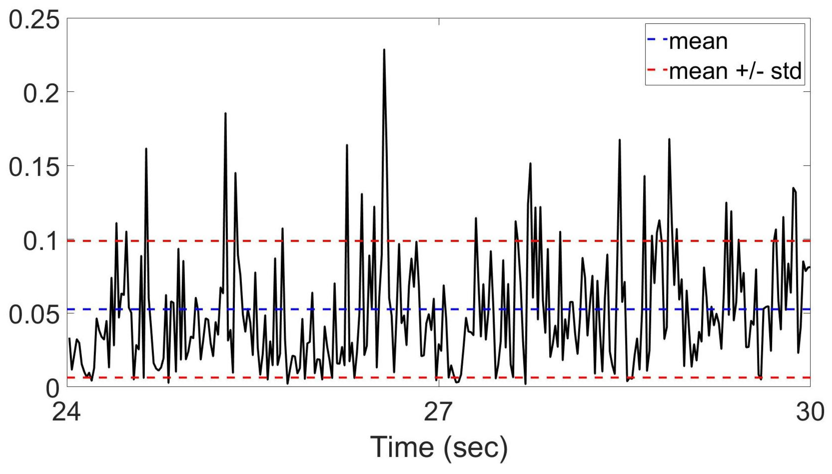
Of importance are also the fluctuations of the instantaneous bed shear stresses near the leading edge of the retaining wall. Figure 14 presents the dimensionless instantaneous bed shear stress value at ( X H , Y H , Z H ) = (0.03, 0.08, 0.07) for a period of six seconds during the data collection time. As shown there, the instantaneous values strongly fluctuate around the mean and they can get as large as four times the mean bed shear stress value at that location. These fluctuations are most likely related to the variation in the frequency of vorticies that are shed from near the toe of the channel bank, and those inside the SSL that originate from the tip of the retaining wall (Figure 6).

3.3. Bimodal Oscillations of the JV1

In order to further characterize the intensity of the JV system along its core, the distribution of the dimensionless TKE estimated as TKE * = u r m s 2 + v r m s 2 + w r m s 2 2 U 0 2 is plotted for different sections within the measurement region (Figure 15). r m s stands for root-mean-square. As mentioned earlier, due to the strong three dimensionality of the flow under investigation, 3D velocity vectors do not accurately define the exact position and size of JV1. In such case, scalar quantities are more useful. Previous studies dealing with the JV system in turbulent junction flows have reported that the JV region is characterized by high turbulence intensity [9,31]. The same observation was made in the present study. More specifically, Figure 15 presents the distribution of TKE* within the sections parallel to the main flow direction which were defined in Figure 10. As shown there, a well-defined region of high TKE* values is present in each of the sections over the channel bank. The amplification of TKE* is primarily due to the large-scale low-frequency oscillations of the instantaneous flow structure associated with the JV system [12,31]. Figure 15 implies that the overall TKE* of the flow, in particular that inside the JV1, increases towards the tip of the retaining wall and then decreases away from it. It is also evident that the high TKE* area progressively gets closer to the retaining wall as it descends down the channel bank. This is consistent with the results obtained from the Q-criterion (Figure 12). The distribution of TKE* on the plane that is perpendicular to the main flow direction, located near the leading edge of the retaining wall is in accordance with observations of Heydari and Diplas [19] (not shown here for the sake of brevity). More specifically, it was observed that a region of high TKE* emanates from the leading edge of the protrusion and extends to the channel bed. The amplification of the TKE* is mainly attributed to the oscillations of the OV (Figure 11a). However, the flow separation from the tip of the flow obstacle, as well as the pronounced flow acceleration due to the abrupt contraction, can also help to elevate the local TKE* value. In agreement with the results presented in Figure 11, as one moves in the upstream direction the overall values of TKE* decrease because the flow exhibits less complexity.
Comparison of the results reported here with previous experimental and numerical studies dealing with junction flows, bridge abutments and spur dikes in particular, suggest marked differences. For instance, Koken and Constantinescu [7] observed C-shaped pockets of high TKE with a double-peak structure inside JV1, near the tip of the spur dike. However, this behavior is not evident in our results presented in Figure 15. Because of significant differences between the present study and above mentioned work, such as the shape of the flow obstructions, the presence of an inclined channel bank in our case, the measurement techniques, and R e number, it is not straight forward to explain the absence of the two peaks in the structure of the high TKE* regions (Figure 15). It is worth noting that the effect of R e number (based on the pier diameter) on the behavior of JV system (e.g., double-peak in TKE structure) has been previously investigated for bridge piers [31].
The large-scale low-frequency oscillations of the JV system are responsible for the elevation of turbulence intensity [9]. More specifically, the JV system alternates quasi-periodically between two modes, namely backflow and zero flow modes. An example of the former condition within the first measurement volume (named M_1 in Figure 2) is illustrated in Figure 16a. It shows the iso-surfaces of the dimensionless Q-criterion at a certain instant of time. This back-flow state is generated when an irrotational patch of fluid with high momentum is carried from near the free surface towards the channel bank by the downflow upstream face of the flow obstruction. There, it tries to maintain its irrotationality. Due to its high momentum, it forms a strong near-wall jet that propagates in the direction opposite to the bulk flow [32]. This pushes the axis of JV1 away from the flow obstruction and transforms its cross-section into an elliptical shape.
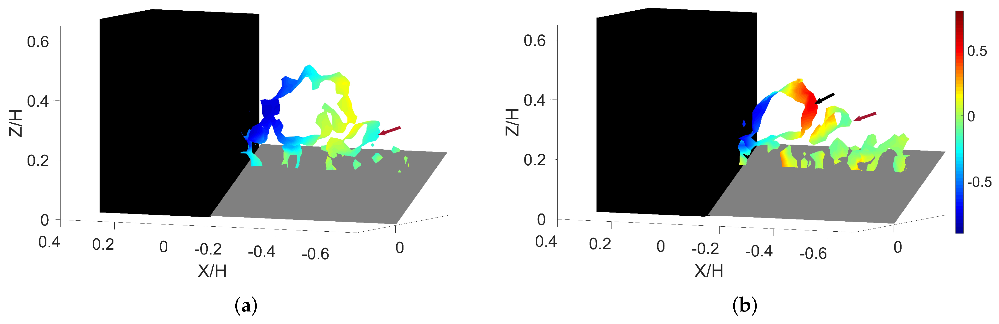
The other extreme flow state (zeroflow mode) at the upstream face of the retaining wall is shown in Figure 16b. It is formed when the path of the previously described reversed flow is blocked by the incoming fluid. This results in a strong vertical ejection of the reversed flow from the boundary along the outer side of JV1, indicated by a black arrow in Figure 16b. In this situation, the JV1 is relatively smaller than that formed during the backflow mode and tends to be closer to the flow obstruction as the incoming flow pushes it downstream. Note that the coherent structure that was detached from the channel bank (Figure 16a), is lifted up during the transition from backflow to zeroflow mode (indicated by a maroon arrow in Figure 16b). See the next section for more details.
The transition from the backflow to the zeroflow mode is initiated by the interaction of JV1 with the bottom boundary layer, which leads to the extraction of BAV with a sign opposite to that inside the JV1 (Figure 17a). A series of representative snapshots of vorticity contours ( ω Y * ), spanning the time interval that starts with the backflow state and ends with the zeroflow mode, are plotted in Figure 17. In consecutive time instants, the BAV strengthens and lifts vertically the JV1 (Figure 17b–e). By this process and the help of incoming flow, JV1 is convected downstream, towards the upstream face of the retaining wall and the complex vortex-to-vortex interactions leads to a rapid breakdown of the JV1 (Figure 17f). Following its destruction, JV1 reorganizes and the entire process is repeated again in an aperiodic manner. Previous studies dealing with sediment transport have suggested that the transition from backflow to zeroflow mode significantly alters the bed shear stress values and greatly contributes to local scouring [33,34]. The onset of BAV is related to the 3D vortex in the close proximity to the wall that exposes it to a strong local adverse pressure gradient. It destabilizes the flow and causes generation of boundary attached vorticities [12,35].
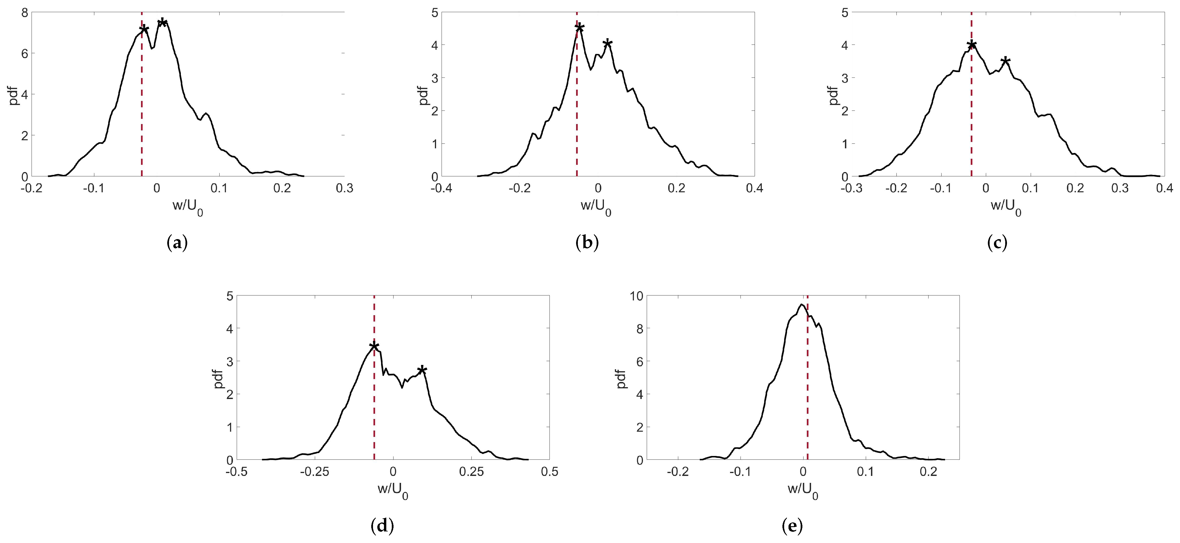
The bimodal behavior of the flow at the upstream face of the retaining wall is further investigated by the examination of the probability density functions (pdf) of the non-dimensional vertical velocity fluctuations just upstream of the core of the JV1. This approach has been used as a robust tool to examine the bimodality of the JV system [8,36]. The zero instantaneous vertical velocity is shown by a dashed line in each of the pdfs included in Figure 18. This helps to establish a meaningful connection between the peaks of the pdfs and each of the modes, namely zeroflow and backflow modes. Identifying if the flow is reversed and directed away from the upstream face of the retaining wall depends on whether the instantaneous vertical velocity is zero, or positive. As shown in Figure 18, the pdf of the vertical velocity fluctuations at various locations over the channel bank depicts a double-peak distribution. During the backflow mode, the reverse flow is almost parallel to the channel bed (Figure 16a). In this case, the wall-normal velocities are close to zero (left peak in Figure 18a–d). Once the zeroflow mode occurs, the wall-normal velocities take positive values. This results in another peak emerging on the right of the first one. Figure 18 also suggests that the velocity difference between the two peaks increases towards the leading edge of the retaining wall (Figure 18d). This explains the increase of TKE* within the JV1 from over the channel bank to near the tip of the retaining wall (Figure 15). As one moves away from the retaining wall (in the spanwise direction), the pdf of the velocity fluctuations shows an unimodal distribution (Figure 18e). A similar behavior was observed within the planes perpendicular to the main flow direction, from near the leading edge of the retaining wall to upstream regions.

3.4. POD Analysis of the Velocity Fluctuations

In an effort to obtain further insights into the underlying flow characteristics, we employed the POD technique that seeks to approximate a high dimensional nonlinear system with a low order (low complexity) model. The POD approach is among the most popular mode decomposition techniques for the extraction and analysis of dominant and energetic turbulent structures. It was first introduced into the turbulence field by Lumley [37]. Recently, Heydari et al. [22] examined the effect of upstream channel bank angle on the turbulent flow characteristics and the associated leading POD modes in the vicinity of the leading edge of a longitudinal structure. The POD decomposes a series of spatial data, the velocity fluctuations field in our case, that are collected at various time instants into a minimum number of modes (basis functions) that are orthogonal to each other. The POD modes are arranged in the order of descending energy content, such that their linear combination approximates the original flow [38]. To estimate the POD modes in the present work, the data obtained with the VPIV system were first arranged in a matrix X form, such that each one of its columns consisted of measurements taken at a specific instant of time, and the number of rows in X was equal to the number of data points within the measurement volume of interest times the number of velocity components (three in our case). Next, the singular value decomposition (SVD) of X was calculated as X = Ψ Σ V , where Ψ and V are unitary matrices characterizing an optimal (in an 2 sense) rank-r truncation of the data matrix X , and Σ is a diagonal matrix characterizing the energy (variance) in each mode. The columns of Ψ contain the spatial structure of each of the POD modes ϕ j ( x ) and the coefficients representing the time evolution of the modes are embedded in the matrix V . The relative importance of the j t h POD mode ϕ j ( x ) in the approximation of the matrix X is determined by its relative energy content:
E j = σ i 2 i = 1 n σ i 2
where σ i are the singular values of matrix X that are ordered in a descending order in the Σ .
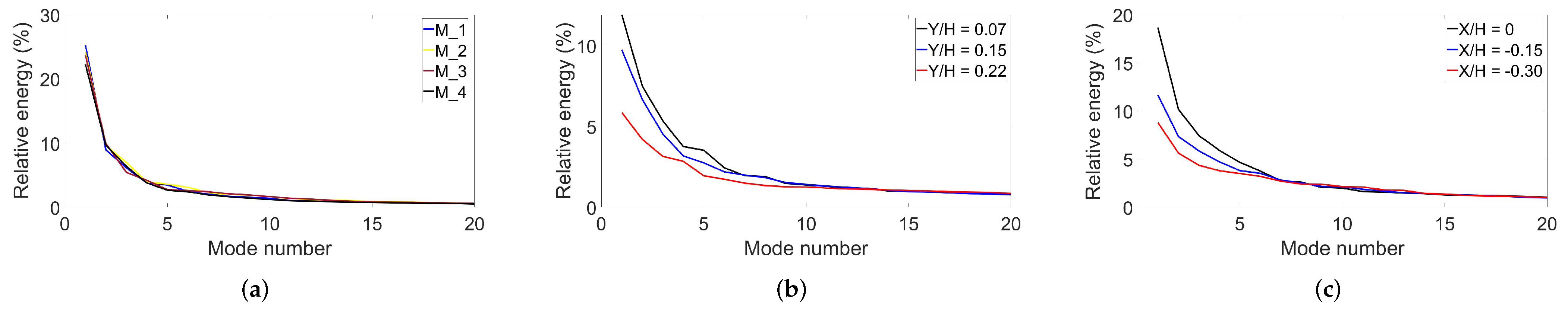
Figure 19a shows the relative energy content of the first twenty energetic POD modes from over the channel bank to near the leading edge of the retaining wall for each of the measurement volumes. The results indicate that in each of the measurement volumes the first eight POD modes capture almost 50% of the total flow energy. The contribution of the first two modes alone, in each of the measurement volumes, adds up to approximately 33%. The relatively low energy content of the first two POD modes, compared to that typically recovered in systems characterized by periodic flow patterns [12,39], suggests the aperiodic behavior of the flow [
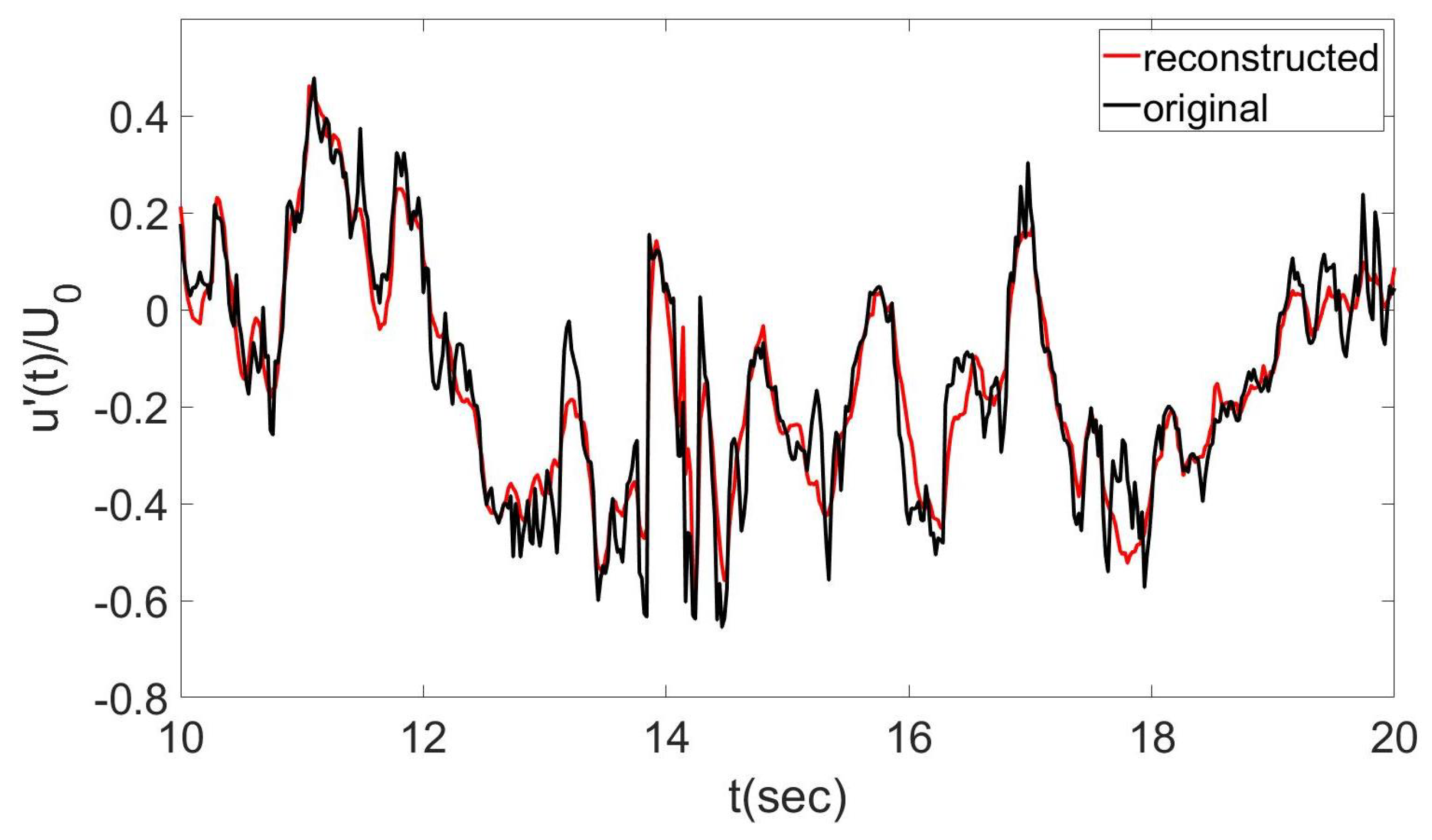
40]. Yet the rapid exponential decay of energy with increasing mode number, implies that the underlying dynamics are controlled by a small number of modes. To examine the validity of this statement, we compared the original streamwise velocity fluctuation time series obtained at a random point within a vertical plane parallel to the mean flow direction over the channel bank with its POD reconstruction using only the first ten POD modes (Figure 20). For a better representation a five seconds time window is shown in Figure 20. The results show that the POD reconstruction can capture in detail the most significant time scales and features of the flow.
Investigation of the energy content of the POD modes within vertical planes parallel to the mean flow direction located beyond the leading edge of the retaining wall indicate that as one moves away from the obstruction, the energy contained in each of the leading POD modes progressively decreases (Figure 19b). This implies that, consistent with the results reported earlier in Figure 10, as the lateral distance (Y direction) from the retaining wall increases, the coherency of the JV system declines and the flow predominantly consists of many small-scale turbulent structures. The same conclusion holds true within the planes perpendicular to the main flow direction ( X < 0 ; Figure 19c). As discussed earlier, the strong downflow around the leading edge of the retaining wall generates the coherent outer vortices. As one moves in the upstream direction, the downflow becomes less significant and thus the outer vortices become less important.
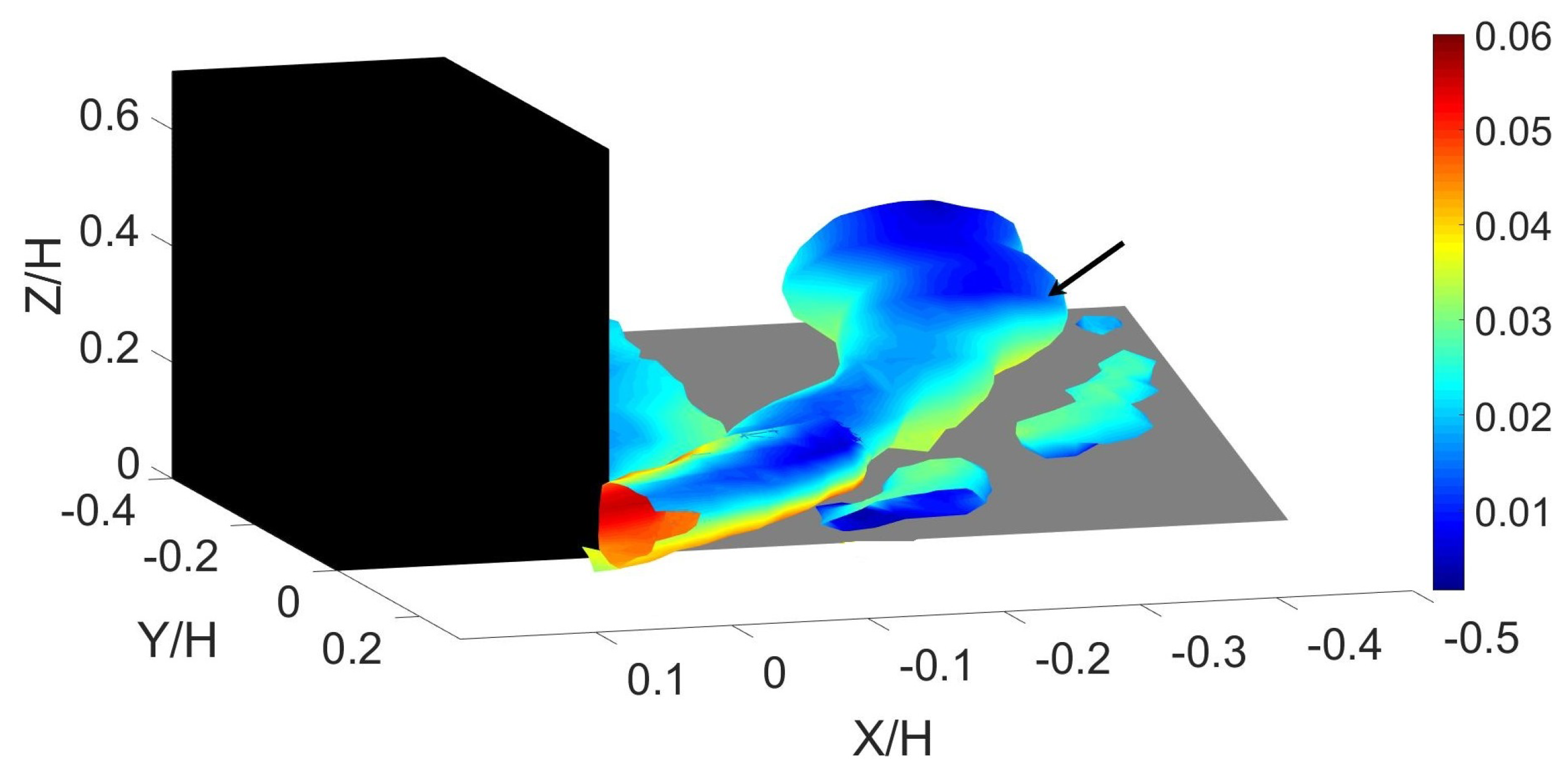
The iso-surfaces of the first POD mode generated by using the Q-criterion are visualized in Figure 21. It shows a well-defined coherent structures that extends from over the channel bank to the tip of the retaining wall (emphasized by a black arrow and is called POD_JV1). Its size, position and orientation implies that this mode is related with the JV1 of the JV system. This POD mode, on average, carries about 24% of the flow energy. The significant values of the | ϕ | 2 , on the iso-surfaces, near the leading edge of the retaining wall, confirms the high-intensity of the JV1 at that location. This is consistent with the results reported in Section 3.2. One important observation is that the path of the POD_JV1 exactly follows the high shear region shown in Figure 13. Therefore, considering its energy content as well, one can conclude that the first POD mode reveals a flow structure that has a significant contribution to the amplification of bed shear stresses and thus to the entertainment of bed particles. Finally, the iso-surfaces in the immediate vicinity of the upstream face of the retaining wall and those upstream of the POD_JV1 are associated with the CV and BAV, respectively.

4. Summary and Conclusions

The turbulent flow characteristics in the vicinity of the leading edge of a retaining wall structure was examined here in order to improve our understanding of the flow physics before the commencement of local scour. This investigation was pursued via the use of a VPIV system. The channel bed in the present work was covered with gravel particles and the flow condition was set to near the initiation of particle motion.
The time-averaged vertical vorticity fields showed the presence of a recirculation region near the upstream face of the retaining wall. This observation verifies the existence of a tornado like structure that extends from the free-surface to near the channel bed. It was also demonstrated that the presence of a relatively mild sloping channel bank ( θ = 28 ), which creates an inclined junction line, does not prevent the formation of the JV system that has been reported in the literature for the case of bridge piers, abutments and other flow obstructions with a horizontal junction line. It was indicated that the position, shape, orientation, and intensity of the primary vortex of the JV system is highly dependent on its distance from the leading edge of the retaining wall. More specifically, the results showed that the JV1 that develops over the channel bank, moves towards the tip of the retaining wall and gradually changes its orientation from being nearly parallel to the upstream face of the obstruction to eventually becoming nearly parallel to the main flow direction at the leading edge of the retaining wall where its intensity is the highest. It was also found that, consistent with previous studies dealing with turbulent junction flows, JV1 oscillates aperiodically between two basic flow states, backflow and zeroflow modes, which were visualized in a 3D space. The bimodality of the JV system was also confirmed via the examination of the pdf of the velocity fluctuations near the core of the JV1. The bimodality of the JV system explains the intermittency and amplification of turbulence within the region occupied by this coherent structure.
The results also specified that the intensity of the bimodal oscillations increases from the area close to the water margin towards the toe of the bank, in the vicinity of the leading edge of the retaining wall. Then a unimodal distribution is recovered beyond this longitudinal structure, in the spanwise direction, within the main channel flow. This explains the higher turbulence intensity inside the JV1 near the leading edge of the retaining wall compared to that over the channel bank. Accordingly, the results indicated that the dominant Reynolds shear stresses along the channel bank nearly follow the path of the JV1 with the highest values occuring near the tip of the retaining wall, where the flow acceleration is the greatest as well. An important observation was the temporal variation of the Reynolds shear stress near the tip of the flow obstruction. It was found that near that location the magnitude of instantaneous shear stress values can reach up to four times the local mean. This was attributed to the fluctuating nature of vorticies inside the SSL that originates from the tip of the retaining wall. It is expected that the flow characteristics described here play a crucial role in the initiation and further development of local scour.
The POD approach provided further insights into the underlying energetic flow characteristics. In particular, the POD results showed that the first and second most energetic POD modes within the measurement volumes over the channel bank contain about 24% and 10% of the total flow energy, respectively. These relatively low energy contributions confirm the aperiodic behavior of the JV system. It was also identified that as the distance from the leading edge of the retaining wall increases (both in the spanwise and upstream directions) the energy contained in each one of the POD modes progressively decreases. This is because the JV system disintegrates in those areas and the flow predominantly consists of many small-scale turbulent structures.
This work elaborated on the important flow features near the upstream face of a retaining wall, confined within an inclined bank, as a limiting case of turbulent junction flows. It also demonstrated the utility of a VPIV systems as a powerful experimental technique for studying complex flow features in the vicinity of in-stream structures that are of interest to sediment transport related phenomena.

Author Contributions

Conceptualization, P.D. and N.H.; methodology, N.H. and P.D.; software, N.H.; validation, P.D. and N.H.; formal analysis, N.H. and P.D.; investigation, N.H. and P.D.; resources, P.D.; data curation, N.H.; writing—original draft preparation, N.H. and P.D.; writing—review and editing, P.D. and N.H.; visualization, N.H.; supervision, P.D.; project administration, P.D.; funding acquisition, P.D. All authors have read and agreed to the published version of the manuscript.

Funding

This research was funded by the National Cooperative Highway Research Program [grant NCHRP-HR 24–36].

Institutional Review Board Statement

Not applicable.

Informed Consent Statement

Not applicable.

Data Availability Statement

The data presented in this study are available on request from the first author.

Conflicts of Interest

The authors declare no conflict of interest.

References

  1. Sukhodolov, A.; Engelhardt, C.; Krüger, A.; Bungartz, H. Case study: Turbulent flow and sediment distributions in a groyne field. J. Hydraul. Eng. 2004, 130, 142–149. [Google Scholar] [CrossRef]
  2. Radspinner, R.; Diplas, P.; Lightbody, A.; Sotiropoulos, F. River training and ecological enhancement potential using in-stream structures. J. Hydraul. Eng. 2010, 136, 967–980. [Google Scholar] [CrossRef]
  3. Sumer, B.; Fredsøe, J. Scour around pile in combined waves and current. J. Hydraul. Eng. 2001, 127, 403–411. [Google Scholar] [CrossRef]
  4. Coleman, S.; Lauchlan, C.; Melville, B. Clear-water scour development at bridge abutments. J. Hydraul. Res. 2003, 41, 521–531. [Google Scholar] [CrossRef]
  5. Dey, S.; Barbhuiya, A. Flow Field at a Vertical-Wall Abutment. J. Hydraul. Eng. 2005, 131, 1126–1135. [Google Scholar] [CrossRef]
  6. Duan, J.; He, L.; Fu, X.; Wang, Q. Mean flow and turbulence around experimental spur dike. Adv. Water Resour. 2009, 32, 1717–1725. [Google Scholar] [CrossRef]
  7. Koken, M.; Constantinescu, G. An investigation of the flow and scour mechanisms around isolated spur dikes in a shallow open channel: 1. Conditions corresponding to the initiation of the erosion and deposition process. Water Resour. Res. 2008, 44, W08406. [Google Scholar] [CrossRef]
  8. Paik, J.; Sotiropoulos, F. Coherent structure dynamics upstream of a long rectangular block at the side of a large aspect ratio channel. Phys. Fluids 2005, 17, 115104. [Google Scholar] [CrossRef]
  9. Devenport, R. Time-dependent and time-averaged turbulence structure near the nose of a wing-body junction. J. Fluid Mech. 1990, 210, 23–55. [Google Scholar] [CrossRef]
  10. Jeon, J.; Lee, J.; Kang, S. Experimental investigation of three-dimensional flow structure and turbulent flow mechanisms around a nonsubmerged spur dike with a low length-to-depth ratio. Water Resour. Res. 2018, 54, 3530–3556. [Google Scholar] [CrossRef]
  11. Melville, B.; Raudkivi, A. Flow characteristics in local scour at bridge piers. J. Hydraul. Res. 1977, 15, 373–380. [Google Scholar] [CrossRef]
  12. Paik, J.; Escauriaza, C.; Sotiropoulos, F. On the bimodal dynamics of the turbulent horseshoe vortex system in a wing-body junction. Phys. Fluids 2007, 19, 045107. [Google Scholar] [CrossRef]
  13. Molinas, A.; Kheireldin, K.; Wu, B. Shear stress around vertical wall abutments. J. Hydraul. Eng. 1998, 124, 822–830. [Google Scholar] [CrossRef]
  14. Kuhnle, R.; Jia, Y.; Alonso, C. Measured and simulated flow near a submerged spur dike. J. Hydraul. Eng. 2008, 134, 916–924. [Google Scholar] [CrossRef]
  15. Kuhnle, R.; Alonso, C. Flow near a model spur dike with a fixed scoured bed. Int. J. Sediment Res. 2013, 28, 349–357. [Google Scholar] [CrossRef]
  16. Rehman, K.; Hong, S.H. Influence of lateral flow contraction on bed shear stress estimation by using measured turbulent kinetic energy. Exp. Therm. Fluid Sci. 2022, 139, 110742. [Google Scholar] [CrossRef]
  17. Launay, G.; Mignot, E.; Riviere, N. Laminar free-surface flow around emerging obstacles: Role of the obstacle elongation on the horseshoe vortex. Eur. J. -Mech.-B/Fluids 2019, 77, 71–78. [Google Scholar] [CrossRef] [Green Version]
  18. Zhang, H.; Nakagawa, H.; Kawaike, K.; Yasuyuki, B. Experiment and simulation of turbulent flow in local scour around a spur dyke. Int. J. Sediment Res. 2009, 24, 33–45. [Google Scholar] [CrossRef]
  19. Heydari, N.; Diplas, P. Flow dynamics in the vicinity of a gravel embedded vertical retaining wall: Conditions corresponding to the initial stages of local erosion. Environ. Fluid Mech. 2020, 20, 203–225. [Google Scholar] [CrossRef]
  20. Khosronejad, A.; Kozarek, J.; Diplas, P.; Hill, C.; Jha, R.; Chatanantavet, P.; Heydari, N.; Sotiropoulos, F. Simulation-based optimization of in-stream structures design: Rock vanes. Environ. Fluid Mech. 2018, 18, 695–738. [Google Scholar] [CrossRef]
  21. Khosronejad, A.; Diplas, P.; Angelidis, D.; Zhang, Z.; Heydari, N.; Sotiropoulos, F. Scour depth prediction at the base of longitudinal walls: A combined experimental, numerical, and field study. Environ. Fluid Mech. 2020, 20, 459–478. [Google Scholar] [CrossRef]
  22. Heydari, N.; Diplas, P.; Nathan Kutz, J.; Sadeghi Eshkevari, S. Modal Analysis of Turbulent Flow near an Inclined Bank–Longitudinal Structure Junction. J. Hydraul. Eng. 2021, 147, 04020100. [Google Scholar] [CrossRef]
  23. Stellmacher, M.; Obermayer, K. A new particle tracking algorithm based on deterministic annealing and alternative distance measures. Exp. Fluids 2000, 28, 506–518. [Google Scholar] [CrossRef]
  24. Koken, M.; Constantinescu, G. Investigation of flow around a bridge abutment in a flat bed channel using large eddy simulation. In Proceedings of the World Environmental And Water Resource Congress 2006: Examining The Confluence Of Environmental And Water Concerns, Omaha, Nebraska, 21–25 May 2006; pp. 1–11. [Google Scholar]
  25. Baker, C.; Taulbee, D.; George, W., Jr. Eddy Viscosity Calculations of Turbulent Buoyant Plumes. In Proceedings of the ASME/AIChE National Heat Transfer Conference, San Diego, CA, USA, 6–8 August 1979. [Google Scholar]
  26. Dargahi, B. The turbulent flow field around a circular cylinder. Exp. Fluids 1989, 8, 1–12. [Google Scholar] [CrossRef]
  27. Koken, M.; Constantinescu, G. Flow and turbulence structure around abutments with sloped sidewalls. J. Hydraul. Eng. 2014, 140, 04014031. [Google Scholar] [CrossRef]
  28. Agui, J.; Andreopoulos, J. Experimental investigation of a three-dimensional boundary layer flow in the vicinity of an upright wall mounted cylinder (data bank contribution). J. Fluids Eng. 1992, 114, 566–576. [Google Scholar] [CrossRef]
  29. Dubief, Y.; Delcayre, F. On coherent-vortex identification in turbulence. J. Turbul. 2000, 1, 011. [Google Scholar] [CrossRef]
  30. Rajaratnam, N.; Nwachukwu, B. Flow near groin-like structures. J. Hydraul. Eng. 1983, 109, 463–480. [Google Scholar] [CrossRef]
  31. Apsilidis, N.; Diplas, P.; Dancey, C.L.; Bouratsis, P. Apsilidis Time-resolved flow dynamics and Reynolds number effects at a wall–cylinder junction. J. Fluid Mech. 2015, 776, 475–511. [Google Scholar] [CrossRef]
  32. Paik, J.; Escauriaza, C.; Sotiropoulos, F. Coherent structure dynamics in turbulent flows past in-stream structures: Some insights gained via numerical simulation. J. Hydraul. Eng. 2010, 136, 981–993. [Google Scholar] [CrossRef]
  33. Escauriaza, C.; Sotiropoulos, F. Lagrangian model of bed-load transport in turbulent junction flows. J. Fluid Mech. 2011, 666, 36–76. [Google Scholar] [CrossRef]
  34. Escauriaza, C.; Sotiropoulos, F. Reynolds number effects on the coherent dynamics of the turbulent horseshoe vortex system. Flow, Turbul. Combust. 2011, 86, 231–262. [Google Scholar] [CrossRef]
  35. Doligalski, T.; Smith, C.; Walker, J. Vortex interactions with walls. Annu. Rev. Fluid Mech. 1994, 26, 573–616. [Google Scholar] [CrossRef]
  36. Kirkil, G.; Constantinescu, G. Flow and turbulence structure around an in-stream rectangular cylinder with scour hole. Water Resour. Res. 2010, 46, W11549. [Google Scholar] [CrossRef]
  37. Lumley, J. Toward a turbulent constitutive relation. J. Fluid Mech. 1970, 41, 413–434. [Google Scholar] [CrossRef]
  38. Berkooz, G.; Holmes, P.; Lumley, J. The proper orthogonal decomposition in the analysis of turbulent flows. Annu. Rev. Fluid Mech. 1993, 25, 539–575. [Google Scholar] [CrossRef]
  39. Gutierrez-Castillo, P.; Thomases, B. Proper Orthogonal Decomposition (POD) of the flow dynamics for a viscoelastic fluid in a four-roll mill geometry at the Stokes limit. J. -Non-Newton. Fluid Mech. 2019, 264, 48–61. [Google Scholar] [CrossRef]
  40. Apsilidis, N.; Diplas, P.; Dancey, C.; Bouratsis, P. Effects of wall roughness on turbulent junction flow characteristics. Exp. Fluids 2016, 57, 1–16. [Google Scholar] [CrossRef]
Figure 1. (a) A schematic of a section of the experimental flume along with the VPIV setup, (b) an upstream looking cross sectional view of the water recirculating flume.
Water 14 03524 g001
Figure 2. A schematic of the measurement volumes located in the vicinity of the upstream face of the longitudinal structure.
Water 14 03524 g002
Figure 3. Dimensionless time-averaged streamwise (<u>*), lateral (<v>*), and vertical (<w>*) flow velocity fields within the representative planes in the immediate vicinity of the retaining wall. The flow direction is shown by a blue arrow.
Water 14 03524 g003
Figure 4. Dimensionless time-averaged velocity fields at (ac) Z H = 0.18 , (df) Z H = 0.32 , and (gi) Z H = 0.49 . The first, second, and third columns show the lateral, streamwise, and vertical velocity components, respectively.
Water 14 03524 g004
Figure 5. Dimensionless time-averaged vertical vorticity fields at (a) Z H = 0.19 , (b) Z H = 0.28 , and (c) Z H = 0.37 from the channel bed.
Water 14 03524 g005
Figure 6. Isosurfaces of the dimensionless time-averaged horizontal vorticity field corresponding to the isovalue of −1.25.
Water 14 03524 g006
Figure 7. (ac) show the < u v > U 0 2 at Z H = 0.17 , 0.22, and 0.26 horizontal planes, respectively.
Water 14 03524 g007
Figure 8. (ac) show the < u w > U 0 2 component at Z H = 0.17 , 0.22, and 0.26 horizontal planes, respectively.
Water 14 03524 g008
Figure 9. The dimensionless instantaneous velocity vectors over the dimensionless (a) spanwise, and (b) streamwise vorticity fields within the representative planes identified in the image inserted in the second row. The flow moves in the positive x-direction.
Water 14 03524 g009
Figure 10. (af) Instantaneous dimensionless velocity vectors laied over the corresponding dimensionless vorticity fields (in the spanwise direction), emphasizing the position and size of JV1, from over the channel bank to within the main channel.
Water 14 03524 g010
Figure 11. (ac) Instantaneous non-dimensional velocity vectors plotted over the ω X * in representative planes perpendicular to the main flow direction to show that OV is pronounced in the immediate vicinity of the retaining wall.
Water 14 03524 g011
Figure 12. Visualization of the mean flow using Q-criterion. (a) shows a 3D view, and (b) illustrates a plan view for the same levels of iso value (2).
Water 14 03524 g012
Figure 13. Distribution of the dimensionless bed mean bed shear stress values, (a) shows a 3D view, and (b) shows a top view along with the isosurfaces of the JV system at isovalue of 1.5.
Water 14 03524 g013
Figure 14. Time series of the dimensionless instantaneous bed shear stress at ( X H , Y H , Z H ) = (0.03, 0.08, 0.07).
Water 14 03524 g014
Figure 15. Distribution of TKE* within the representative vertical sections, parallel to the main flow direction, (ad) over the channel bank and (e,f) within the main channel. The location of the sections parallel to the main flow direction shown here was defined in Figure 10.
Water 14 03524 g015
Figure 16. Instantaneous iso-surfaces of the dimensionless Q-criterion in a representative section over the channel bank at the upstream face of the retaining wall showing the (a) backflow, and (b) zeroflow modes of the JV1 vortex. The color coding corresponds to the vertical velocity component.
Water 14 03524 g016
Figure 17. (af) Instantaneous spanwise vorticity fields showing the transition over−time from backflow mode to zeroflow mode within a representative plane, that is vertical and is in the streamflow direction, located at Y H = 0.28 . The time interval between consecutive images is 0.02 s.
Water 14 03524 g017
Figure 18. (ae) The pdfs of the vertical velocity fluctuations just upstream of the core of JV1 (in the mean flow) within the planes identified in Figure 10.
Water 14 03524 g018
Figure 19. The relative energy content of the first twenty POD modes within (a) the individual measurement volumes over the channel bank, (b) vertical planes aligned with the flow and located beyond the retaining wall in the spanwise direction, and (c) vertical planes perpendicular to the main flow direction within the main channel.
Water 14 03524 g019
Figure 20. Reconstruction of the dimensionless streamwise velocity fluctuations (red line) using the first ten POD modes, compared to the original data (black solid line).
Water 14 03524 g020
Figure 21. The first energetic POD mode. The color coding represents the Euclidean norm of the modes calculated as | ϕ | 2 = ϕ u 2 + ϕ v 2 + ϕ w 2 . Note that ϕ u , ϕ v and ϕ w are the POD sub-modes associated with the streamwise, lateral, and vertical velocities, respectively.
Water 14 03524 g021
Table 1. Experimental flow and boundary conditions.
H U 0 S u s F r Re u s / u cr
(m)(m/s)(%)(m/s)---
0.180.570.140.050.43282,4300.90
H = flow depth; U0 = approach depth-averaged flow velocity; S = channel bed slope; us = shear velocity = τ 0 ρ ; τ 0 =   γ H S = mean bed shear stress; γ = specific weight of water; F r =   U 0 g H = Froude number; g = gravitational acceleration; R e =   U 0 4 R v = Reynolds number; R   =   A P = hydraulic radius; A = cross-sectional area; P = wetted perimeter; v = kinematic viscosity of water; ucr = critical shear velocity.
Publisher’s Note: MDPI stays neutral with regard to jurisdictional claims in published maps and institutional affiliations.

