Article

Analysis of Floating Macroalgae Distribution around Japan Using Global Change Observation Mission-Climate/Second-Generation Global Imager Data

1
Graduate School of Advanced Science and Technology, Hiroshima University, Higashi-Hiroshima 739-8527, Japan
2
Fisheries Resources Institute, Japan Fisheries Research and Education Agency, Hatsukaichi 739-0452, Japan
3
Fisheries Resources Institute, Japan Fisheries Research and Education Agency, Yokohama 236-8648, Japan
*
Author to whom correspondence should be addressed.
Water 2022, 14(20), 3236; https://doi.org/10.3390/w14203236
Submission received: 13 July 2022 / Revised: 12 September 2022 / Accepted: 11 October 2022 / Published: 14 October 2022
(This article belongs to the Section Oceans and Coastal Zones)

Abstract

:
Floating macroalgae information is required to manage coastal environments and fishery resources effectively. In situ observations and analyses can result in under-sampling, thereby challenging the comprehension of the floating macroalgae abundance and spatiotemporal alterations. This study reports the spatiotemporal variation of floating macroalgae distribution around Japan from 2018 to 2021 using Global Change Observation Mission-Climate/second-generation Global Imager data. We employed the floating algae index (FAI) scaled from local ocean FAI to minimize the effect of spatial variation in ocean color. Fractional macroalgae coverage in a pixel was determined using a linear unmixing algorithm with lower and upper thresholds. The lower threshold was determined using the cumulative frequency of the scaled FAI, and the upper threshold was modified based on the more precise Sentinel-2 data. The results revealed that monthly macroalgae coverage varies spatially and seasonally, peaking in the spring and summer in the southwestern area. The macroalgae distribution particularly expanded from the East China Sea to west Japan during spring. In 2018–2021, the total biomass of the offshore floating macroalgae was estimated to be 8880–133,790, 8460–141,900, 3910–70,380, and 4620–61,870 tons. The findings of this study validated the empirical knowledge about specific locations and can serve as a reference to analyze temporal and spatial variations in future studies.

1. Introduction

This study investigated the temporal variation in floating macroalgae (seaweed) distribution around Japan using satellite remote sensing. Floating macroalgae are prevalent across global coastal waters, but certain macroalgae blooms are especially well-known due to their magnitude; for example, S a r g a s s u m in the Sargasso Sea (and the Caliban Sea and the Gulf of Mexico) and macroalgae blooms of U l v a species off the coast of Qingdao (the Yellow Sea), China (often referred to as green tides) (e.g., [1,2]). High quantities of floating macroalgae and their beaching have major implications on ecosystems and economies [3,4]. On the other hand, floating macroalgae provide a habitat for aquatic animals, including fishes that use them as breeding grounds or travel with macroalgae rafts as juveniles. Juvenile yellowtail (amberjack) accompanying S a r g a s s u m rafts are caught and bred for human consumption; thus, floating macroalgae play an essential role in fisheries. Additionally, floating macroalgae are potential blue carbon sources due to their accumulation on the deep seafloor although the contribution to deep-sea carbon sequestration is smaller than that from non-floating macroalgae and seagrass in coastal areas [5]. The presence, distribution, abundance, advection (movement), and settling of floating macroalgae (and their temporal variation) must be explored to effectively manage coastal environments and fishery resources and for blue carbon strategy.
Satellite remote sensing employing multiple indices is a unique approach for analyzing floating macroalgae distribution over a wide area (e.g., [6]). These indices use the spectral difference between red and near-infrared bands because floating macroalgae have a red edge in their reflectance spectrum. Two examples are the maximum chlorophyll-a index, and the normalized difference vegetation index (NDVI) (e.g., [7,8]). Recently, Hu (2009) proposed the floating algae index (FAI) as an alternative to NDVI [9]. F A I is the difference between near-infrared reflectance and the red-to-shortwave infrared baseline. Hu (2009) suggested that the baseline subtraction makes FAI less sensitive to environmental and observational changes than NDVI. Since the proposal by Hu (2009), FAI has been widely used to detect floating macroalgae with data from Moderate Resolution Imaging Spectroradiometer (MODIS) onboard Terra/Aqua satellites. Additionally, macroalgae detection may have been improved by removing inherent spatial variations caused by ocean color or atmospheric influences from an original index map [10].
In December 2017, the Japan Aerospace Exploration Agency (JAXA) launched the Global Change Observation Mission-Climate (GCOM-C), carrying the second-generation Global Imager (SGLI) [11]. The GCOM-C/SGLI has 19 observation channels with wavelengths ranging from 380 to 12,000 nm (visible to thermal infrared bands). The visible and infrared channels have 1,150 and 1,400 km swath widths and 250 or 1000 m spatial resolutions, respectively, depending on the channel. About every two days, GCOM-C/SGLI visits and makes observations. Data on channel reflectance and various products derived from them are available. Figure 1 depicts a GCOM-C/SGLI RGB image of the distribution of green tide off the coast of Qingdao, China. The FAI computation requires red, near-infrared, and shortwave infrared reflectance data [9]. GCOM-C/SGLI has channels with a 250 m spatial resolution for these wavelength bands, allowing FAI to be acquired with a 250 m spatial resolution. The GCOM-C/SGLI FAI is available through the FAI Viewer operated by JAXA Satellite Monitoring for Environmental Studies (JASMES; https://www.eorc.jaxa.jp/JASMES/FAI/index.html (accessed on 13 October 2022)). Figure 1b shows GCOM-C/SGLI FAI of the same data as Figure 1a. GCOM-C/SGLI captures floating macroalgae events (such as U l v a species in Figure 1) with improved spatial resolution. However, the algorithm theoretical basis document (ATBD) of GCOM-C/SGLI FAI [12] mentions that an original GCOM-C/SGLI FAI dataset exhibits high FAI around clouds and lands, which may lead to mis-classifications. Because GCOM-C/SGLI is a relatively new satellite/sensor and there is the issue described in ATBD, there is currently no literature demonstrating how to apply GCOM-C/SGLI FAI to a floating macroalgae study.
Due to their proximity to the coastal environment and fisheries, floating macroalgae have been explored in Japanese coastal areas for decades (e.g., [13]). In Japan, floating macroalgae research involves field observations, cruise ship samplings, and laboratory experiments (e.g., [14,15]). In recent years, cruise-ship-based observational studies [16,17] have identified a significant amount of S a r g a s s u m in the East China Sea, with part of it flowing west of Japan. Local fishery institutions retain records on sampled floating macroalgae, but this may not be sufficient to estimate the distribution, total quantity, seasonal and interannual changes, or spatial variations because in situ ship observations sample floating macroalgae in limited areas and times. While satellite remote sensing cannot provide as much detailed and precise information as field observations and sampling, it can provide an overview of floating macroalgae across a vast area. For example, Qi et al. (2017) used MODIS data to determine the amount of S a r g a s s u m in the East China Sea, with a mean area density of about 0.3% [18].
As an application of satellite remote sensing to a floating macroalgae study, this paper uses GCOM-C/SGLI data to explore the distribution and temporal variation of floating macroalgae around Japan from 2018 to 2021. We modified the original GCOM-C/SGLI FAI data in this study to improve floating macroalgae detection. In addition, higher-resolution Sentinel-2/MSI data were used to evaluate and tailor GCOM-C/SGLI FAI data estimates. Using the modified GCOM-C/SGLI FAI data, we clarified the distribution, amount, and temporal variation of floating macroalgae around Japan. It should be noted that microalgae have similar reflectance spectra to that of floating macroalgae; thus, FAI (and other similar indices) would not distinguish between the two algae types. While we assume that microalgae are found in inland and nearshore shallow water, we exclude pixels near the land (and inland waters) from analysis as described in Section 2; thus, we consider that macroalgae contribute to high FAI in this study. The summarized data in this study can be a reference to validate the empirical knowledge about floating macroalgae obtained by several local fishery institutions and for future temporal and spatial variation investigations.

2. Materials and Methods

This study clarifies the spatiotemporal variation of floating macroalgae distribution around Japan by using FAI derived from the GCOM-C/SGLI data. To reduce the effects of spatial resolution, we use a method that tailors the GCOM-C/SGLI FAI by the FAI obtained from Sentinel-2/MSI with a higher spatial resolution. In this section, we present the derivation of FAI (Section 2.1), a new index based on FAI to improve macroalgae detection (Section 2.2), and how the macroalgae area is computed (Section 2.3) and binned (Section 2.4).

2.1. Floating Algae Index (FAI)
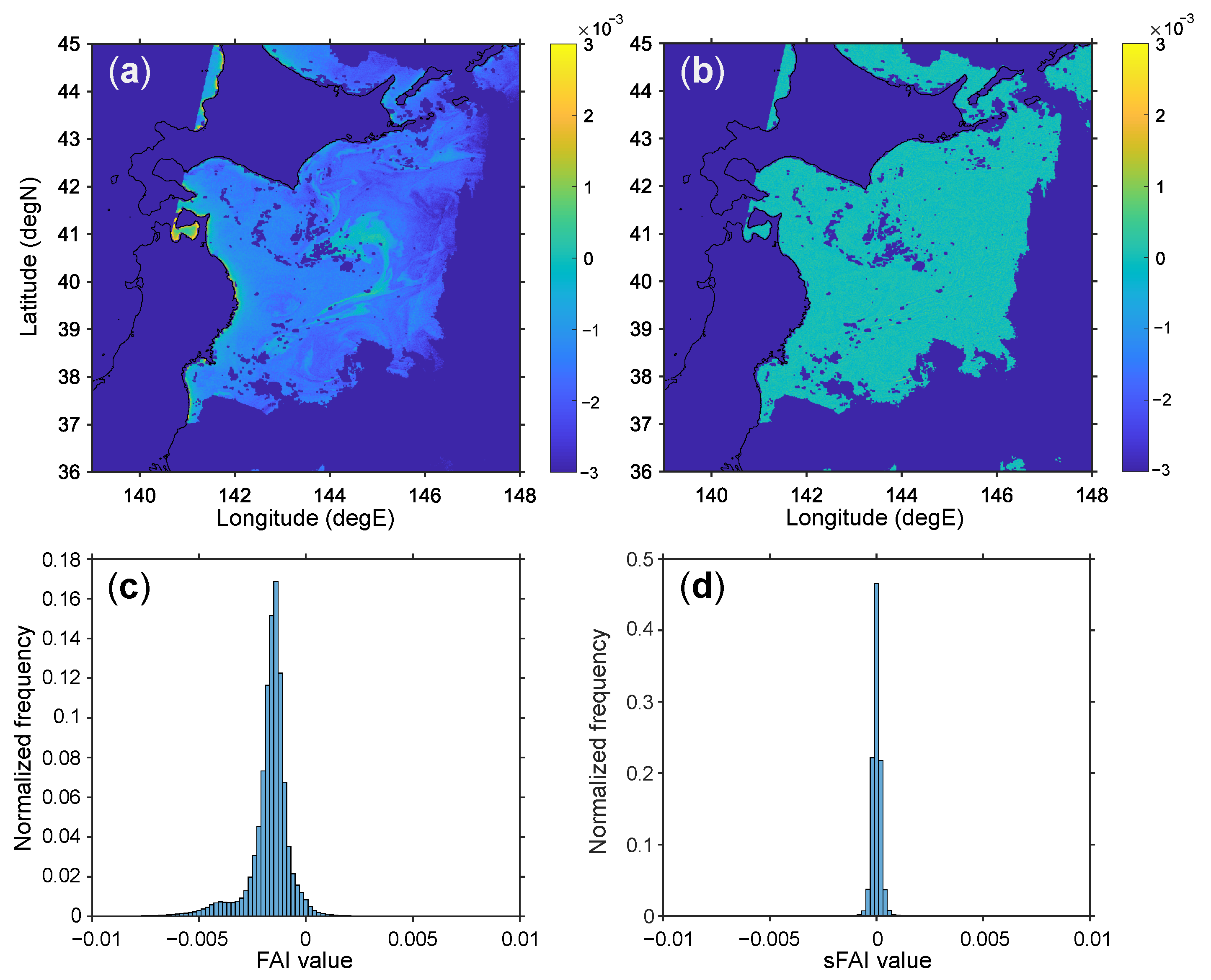
According to Hu (2009), FAI is the difference between near-infrared reflectance and a linear baseline between red and shortwave infrared bands [9]. FAI is calculated as
FAI = R NIR R NIR ,
R NIR = R RED + R SWIR R RED λ SWIR λ RED λ NIR λ RED ,
where R is the Rayleigh-corrected reflectance, λ is the wavelength; the subscripts NIR, RED, and SWIR represent the near-infrared, red, and shortwave infrared spectral bands, respectively. R NIR represents the baseline reflectance at λ NIR . Therefore, FAI is derived from the linear combination of red, near-infrared, and shortwave infrared reflectance.
JAXA provides a GCOM-C/SGLI-derived FAI product. According to ATBD for GCOM-C/SGLI FAI [12], the FAI was calculated using the following equation:
FAI = ρ 865 0.3399 ρ 1630 0.6356 ρ 672 ,
where ρ λ indicates the reflectance at wavelength λ in nanometers (i.e., the subscript number indicates wavelength in nanometers), and the reflectance ρ at each wavelength was calculated using the following equation:
ρ = ρ TOA ρ m / t m ,
where ρ TOA is top-of-atmosphere reflectance, ρ m is molecular scattering, and t m is transmittance. The coefficient of Equation (3) was determined using the approach described by Flouin et al. (2006) [19] to minimize the aerosol effect [12].
We used a 250 m spatial resolution GCOM-C/SGLI product containing FAI data for Japan (area bounded by 123 E–150 E and 23 N–50 N). The area covered by this product is depicted in Figure 2. The daily FAI products for the years 2018 to 2021 were downloaded from the JASMES ftp server. The original FAI result masked land or cloud pixels. However, we discovered that some pixels with a high FAI due to clouds were not successfully masked. As a result, we used other products to assess the data quality, such as the cloud flag, and used only the pixel having the highest quality by the QA flags of these products. Furthermore, the ATBD of GCOM-C/SGLI FAI [12] mentions that high FAI can appear near cloud or land pixels due to small misregistration across channels; consequently, we concluded that a pixel was invalid if there were invalid pixels (due to land or cloud) within 9 × 9 pixels centered on that pixel. The spatial variation in floating macroalgae appearance is also valuable information. Therefore, we divided the ocean around Japan into the subareas depicted in Figure 2 to characterize the variation of floating macroalgae. The subareas were determined based on the subarea divisions by Fisheries Agency, Japan, to establish fishing zones.

2.2. Scaling FAI

The FAI value of each pixel was used to determine whether the sea surface corresponding to a focusing pixel contained floating macroalgae. Researchers have applied a fixed threshold to make this determination. However, despite the presence or non-presence of floating macroalgae, the FAI value varies spatially due to spatially-varying atmospheric or ocean color influences (for example, see Figure 3 in [20]); thus, finding an appropriate threshold is difficult. Applying a fixed and constant threshold to data, where FAI changes spatially due to atmospheric or ocean color effects, might increase instances in which algae-containing pixels are incorrectly classified as non-algae-containing pixels and vice versa. The atmospheric or ocean color effects can be minimized by subtracting the local ocean’s FAI from the FAI of the focusing pixel [20,21], where the local ocean FAI reflects the seawater (non-algae) pixel near the focusing pixel, because these effects are reasonably consistent across several pixels. Garcia et al. [20] applied this concept to NDVI and named it the scaled algae index (SAI or SAI NDVI ). Namely, SAI is the difference in NDVI between the targeted pixel and the local ocean. Following the naming rule of Garcia et al. [20], we used the term “scaled” to refer to the difference between the FAI of the focusing pixel and the local ocean as scaled FAI (sFAI). Thus, the sFAI was expressed as
sFAI = FAI FAI lo ,
where FAI lo indicates the local ocean’s FAI. When there were no floating macroalgae in a specific area, this pixel’s sFAI value approached zero regardless of the atmospheric or ocean color effects, whereas the sFAI of the algae-containing pixels became significantly positive.
Following Garcia et al. [20], the local ocean FAI ( FAI lo ) was calculated using the median FAI value in the sub-image containing the focusing pixel (i.e., image kernel). Local ocean FAI is meaningful only if the kernel contains more non-algae pixels than algae pixels. Therefore, the image kernel size must be sufficiently large to contain more non-algae pixels than algae pixels; in this case, the median FAI of the focusing kernel represents a non-algae (i.e., seawater) pixel. On the other hand, a reduced kernel size effectively eliminates spatial FAI variance. We decided to use a 21 × 21 kernel, which was the smallest size accepted by Garcia et al. [20]. Figure 3 shows an example of FAI and sFAI maps on a day. The high spatial variance in FAI (Figure 3) was likely due to red-band reflectance and mesoscale ocean variability. Such spatial variation was negligible (not visible) in sFAI (Figure 3b). Histograms (Figure 3c,d) reveal that FAI had a long-tailed distribution, whereas sFAI had near-zero values with a narrower range. The standard deviations of the FAI and sFAI values were about 1.0 × 10 3 and 2.1 × 10 4 , respectively.
When macroalgae covered only a part of a pixel, the sFAI value did not increase significantly. With a constant threshold for such pixels, algae-containing pixels were misclassified as non-algae-containing pixels and vice versa. It was difficult to reduce both cases simultaneously. Garcia et al. [20] investigated the sensitivity of macroalgae detection to multiple thresholds (99.5%, 99.6%, 99.7%, 99.8%, 99.9%, and 99.99%) in the cumulative frequency of sFAI (SAI NDVI in their paper). This study followed the approach of Garcia et al. [20], but considered three thresholds: sFAI values at 99.7%, 99.9%, and 99.99% in the cumulative frequency. We also decided that the sFAI of the algae-containing pixel must be greater than 0.0015, which is larger than multiples of the standard deviation of the sFAI histogram. For example, the standard deviation of sFAI in Figure 3d was 2.1 × 10 4 . Therefore, the threshold was greater than either 0.0015 or above the three thresholds. Based on this threshold (termed as sFAI min ), all pixels in the around-Japan area (Figure 2) were classified into algae-containing pixels, algae-free pixels (non-algae pixels), and invalid (such as cloud and land) pixels.

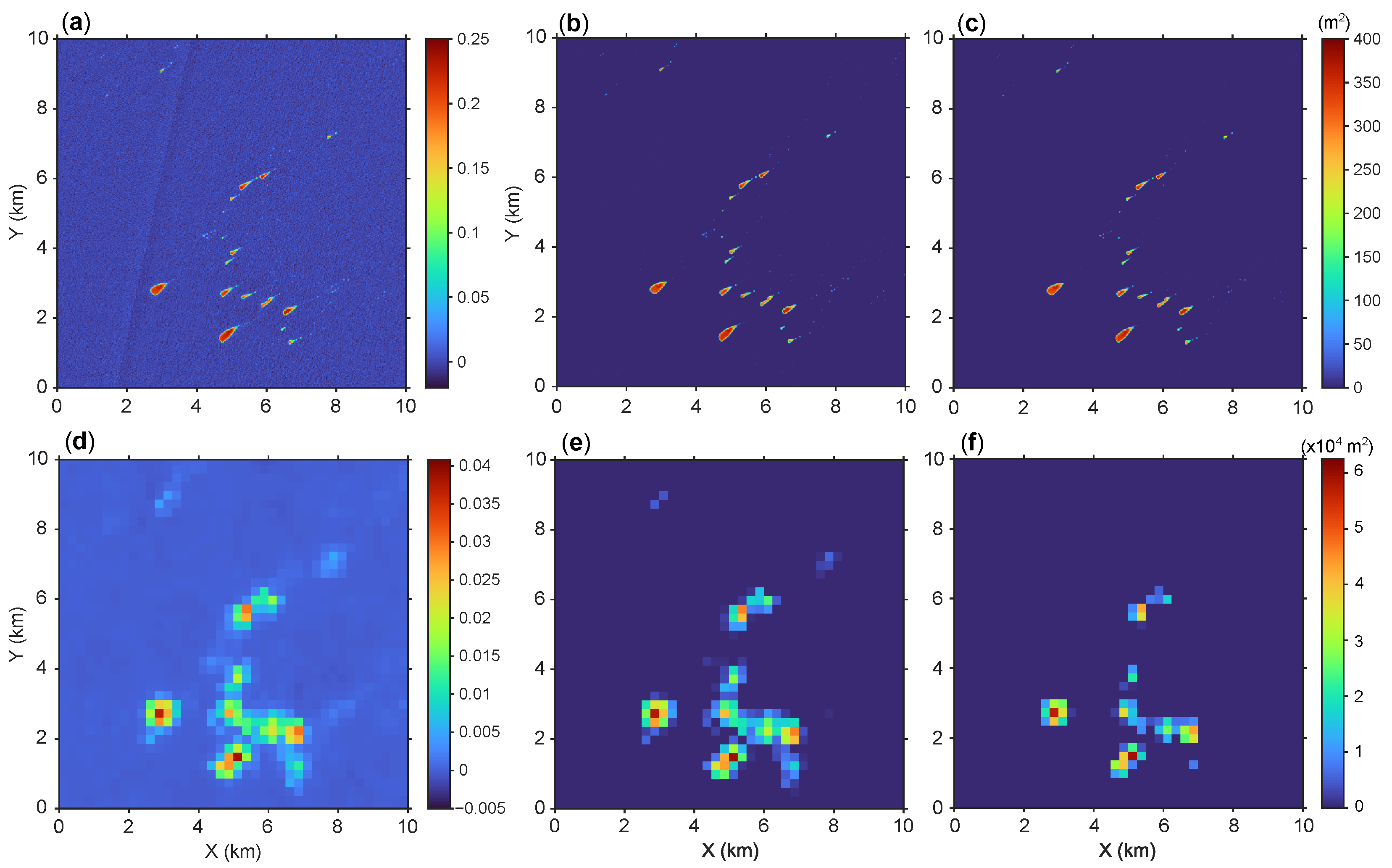
2.3. Algae Area Estimation

The fractional macroalgae coverage within an algae-containing pixel was determined using the linear unmixing method [20,21]:
α = sFAI sFAI min sFAI max sFAI min ,
where α is the fractional macroalgae coverage of the pixel of interest, sFAI min is the macroalgae detection threshold (sFAI values at 99.7%, 99.9%, or 99.99% in the cumulative frequency), and sFAI max is the upper bound of the sFAI value. By applying the linear unmixing method of Equation (6), we obtained the fractional coverage α of a focusing pixel in a range of 0–1. Note that if sFAI of a focusing pixel was smaller than sFAI min or larger than sFAI max , α were set to zero and one, respectively. The total macroalgae area of the pixel was calculated by multiplying each pixel area ( 250 × 250 m 2 ) by α .
High spatial resolution images can capture the floating algae blooms more precisely, allowing for more accurate area estimations. We assessed the precision of the GCOM-C/SGLI sFAI estimate of floating macroalgae area using Sentinel-2/MSI data and tuned an acceptable sFAI max for GCOM-C/SGLI sFAI. The GCOM-C/SGLI and Sentinel-2/MSI data observing a part of the East China Sea on 7 May 2020 were used for this evaluation. Sentinel-2/MSI FAI was calculated using reflectances in bands 4, 8a, and 11 at 10, 20, and 20 m spatial resolutions, respectively. The spatial resolution of Sentinel-2/MSI FAI (and sFAI) in this investigation was 20 m as the band 4 reflectance data (10 m) was down-sampled to fit the other two reflectance data. Figure 4a,d shows sFAI images of Sentinel-2/MSI and GCOM-C/SGLI (a part of the area for the evaluation data), respectively. Sentinel-2/MSI could effectively capture the floating macroalgae shapes with precision (Figure 4a). By contrast, GCOM-C/SGLI captured the floating macroalgae in blurred shapes (Figure 4d). Below, we describe how sFAI max for GCOM-C/SGLI was calculated using the Sentinel-2/MSI result.
Due to the high spatial resolution of Sentinel-2/MSI sFAI (Figure 4a), massive macroalgae blooms (red colored area) were composed of many pixels. Sentinel-2/MSI had an sFAI value of around 0.25 in some pixels but 0.22 in the center of large macroalgae patches; thus, a sFAI max of 0.22 would be reasonable for Sentinel-2/MSI. Figure 4b,c present macroalgae area in each pixel, calculated using Equation (6) and Sentinel-2/MSI pixel area ( 20 × 20 m 2 ) with sFAI min at 99.7 % (Figure 4b) and 99.9 % (Figure 4c). The total macroalgae area of Sentinel-2/MSI sFAI in the test area was about 1.289 and 1.062 km 2 for sFAI min of 99.7 % and 99.9 % , respectively. The highest GCOM-C/SGLI FAI value is 0.0408, making it a candidate for sFAI max . When we set 0.0408 for sFAI max and computed the macroalgae area using Equation (6), we obtained 3.331 and 2.049 km 2 for sFAI min at 99.7 % and 99.9 % , respectively (Figure 4e,f). Despite missing small patches of floating macroalgae (especially in the case of sFAI min = 99.9%), GCOM-C/SGLI sFAI produced two to three times more macroalgae area than Sentinel-2/MSI sFAI. Thus, using GCOM-C/SGLI sFAI with sFAI max of 0.0408 possibly overestimated macroalgae area. When we set 0.1 to GCOM-C/SGLI sFAI max , which was approximately 2.5 times of 0.0408, we obtained macroalgae area of 1.299 and 0.761 km 2 for sFAI min at 99.7 % and 99.9 % , respectively. From this comparison, we assumed sFAI max for GCOM-C/SGLI would be between 0.0408 to 0.1, and we considered 0.04, 0.07, and 0.1 in the following analysis. Here, we rounded 0.0408 down to 0.04 and added 0.07 as an intermediate number. So, we computed the total macroalgae area using combinations of three sFAI max (0.04, 0.07, and 0.1) and three sFAI min ( 99.7 % , 99.9 % , and 99.99% in the cumulative frequency of sFAI). The absence of ground truth data made the selection and validation of optimal values of sFAI min and sFAI max difficult; thus, we assumed the variation of the estimated macroalgae area due to sFAI max and sFAI min (i.e., sensitivity to sFAI max and sFAI min ) to be the possible macroalgae area range.

2.4. Algae Area Binning

After obtaining macroalgae coverage in each pixel, we binned the data and generated the monthly mean distribution of macroalgae on 0 . 5 × 0 . 5 grids following the method of Wang and Hu [21] for the visualization of floating macroalgae distribution maps. Using the same grid size [21] (i.e., 0 . 5 × 0 . 5 ), we compared our results with those of Wang and Hu [21]. The monthly mean fractional macroalgae coverage in each 0 . 5 × 0 . 5 grid was calculated using the following equation [21]:
f = 1 N i α i ,
N = N A + N W ,
where f is the monthly mean fractional macroalgae coverage, N A and N W are the number of algae-containing and algae-free pixels in a 0 . 5 × 0 . 5 grid and within a focusing month, respectively, and α i = 0 for algae-free pixels. We excluded invalid pixels for the calculation.

3. Results and Discussion

Figure 5 depicts the temporal variation of the macroalgae area around Japan between 2018 and 2021. The monthly mean macroalgae area in each pixel was calculated by multiplying the grid area with the monthly mean fractional coverage f. Then, we summed the computed monthly mean macroalgae area over all the subarea shown in Figure 2. The estimated macroalgae area varied seasonally, with the area being more extensive in the spring and summer and smaller in the autumn and winter. The floating macroalgae area also varied interannually, with spring 2018 and 2019 larger than spring 2020 and 2021. Several local fishery institutions have noted similar interannual variations, although they monitor floating macroalgae in limited areas and times. The macroalgae area fluctuated between 1 and 20 km 2 in 2018 and 2019 and between 1 and 10 km 2 in 2020 and 2021 (for sFAI min = 99.7% and sFAI max = 0.04; blue solid line). As we see later in Figure 6, the vast area of floating macroalgae in spring was associated with the transportation of floating macroalgae from the East China Sea.
When many floating macroalgae were detected, the sensitivity of the macroalgae area to sFAI min or sFAI max was relatively high, particularly in summer. In July and August 2019 (and 2018), the estimated macroalgae area with sFAI min = 99.7 % (blue lines) and sFAI min = 99.99 % (orange lines) varied significantly. The estimated macroalgae areas for sFAI min = 99.7 % ranged from 5–20 km 2 (blue lines), but for sFAI min = 99.99 % , the macroalgae areas were less than 2–3 km 2 (orange lines) for all sFAI max . The estimated macroalgae area during these two months was more sensitive to sFAI min than the sFAI max . By contrast, in April and May 2019 (and 2018), the use of sFAI min = 99.99 % resulted in large macroalgae area estimates, and the discrepancies between the results with sFAI min = 99.99 % and with sFAI min = 99.7 % were fewer (i.e., less sensitivity to sFAI min ) than those in July and August. We discuss this seasonal variation below.
In the spring, less sensitivity to sFAI min indicates the proximity of the sFAI values at 99.7%, 99.9%, and 99.99% of the cumulative frequency and that there were many pixels having similarly high sFAI values. This indicates that there were pixels that were not classified as algae-containing pixels even though they had similarly high sFAI values. Therefore, in the spring, the use of 99.9 % and 99.99 % sFAI min would underestimate the macroalgae area. Even 99.7 % sFAI min might be too high for evaluating the macroalgae area, and it is possible that the macroalgae area were higher than the estimates shown in Figure 5. In the summer, on the other hand, high sensitivity to sFAI min suggested that sFAI values at 99.7%, 99.9%, and 99.99% cumulative frequency were clearly distinct. In this case, an appropriate sFAI min value would exist between the sFAI values at 99.7% and 99.99%, and the value for sFAI min could be higher than the sFAI value at 99.7 % to narrow the possible range of the macroalgae area estimates. Given the difficulties in determining the optimal sFAI min value, we used three sFAI min values and interpreted the scatter of the results as the range of the floating macroalgae area. However, the optimal sFAI min values to provide the possible range of macroalgae area (e.g., at 99.7%, 99.9%, and 99.99% of the sFAI cumulative frequency) varied with time. Lower and higher values of sFAI min than that at 99.7% in the cumulative frequency of sFAI might be preferred in spring and summer, respectively, to provide a more reasonable possible range of the floating macroalgae estimates.
When the macroalgae area estimates were small (i.e., during autumn and winter), the difference between sFAI min = 99.7 % (blue) and sFAI min = 99.9 % (red) was either absent or insignificant. The reason for this was that the sFAI values at 99.7% and 99.9% cumulative frequency for these months were less than 0.0015 (the lower limit for sFAI min ; see Section 2.2); thus, sFAI min = 0.0015 was chosen rather than the values determined by 99.7% and 99.9% in the cumulative frequency in both the macroalgae area estimates. Therefore, small algal area estimations showed no difference between sFAI min = 99.7 % and sFAI min = 99.9 % .
Figure 6 shows the monthly-binned spatial distribution of fractional floating macroalgae coverage (in 0 . 5 × 0 . 5 grids) in 2019 and 2020, with sFAI min = 99.9% and sFAI max = 0.07. Note that, as the color was specified on 1024 levels, pixels with less than 0.0001% (i.e., 0.1 / 1024 ) binned fractional coverage remained white in the color plot. Seasonal variation of floating macroalgae distribution is also found in Figure 6 together with some spatial characteristics. Floating macroalgae were found all over Japan (both offshore and along the coast), but they were most prevalent in the East China Sea during the spring season (March to May), accounting for the vast macroalgae area shown in Figure 5. The maximum fractional coverage in the East China Sea was 0.1 % (on 0 . 5 × 0 . 5 grids), which was comparable to that in the Central Western Atlantic [21], but smaller than that in the East China Sea in 2017 (0.3%; [18]). Floating macroalgae in the East China Sea appeared to be in a decreasing trend for the recent five years. The massive amount of floating macroalgae in the East China Sea may not be the massive green tide ( U l v a ) found off the coast of Qingdao, China, but may be S a r g a s s u m ( S . h o r n e r i ) [17,18]. It has been reported that S . h o r n e r i from the East China Sea was transported to the west coast of Japan during the spring season (e.g., [22]). Figure 6 depicts the expansion of the massive macroalgae area to west Japan in the spring. The floating macroalgae from the East China Sea appeared to have been transported to the Japan Sea and the Pacific Ocean in the spring of 2019, but not in 2020.
Low-coverage (blue-colored area) floating macroalgae increased south of Japan during the summer, although the results in July and August were somewhat inconclusive, as depicted in Figure 5. Some low-coverage macroalgae detections in summer were associated with clouds or hazy conditions that could not be masked successfully, but it does not explain why the number of low sFAI pixels increased throughout the summer. The increases of floating macroalgae in south of Japan in summer may partly be explained by the presence of tropical (subtropical) S a r g a s s u m species, whose floating macroalgae formation occurs mainly during summer; for example, Yamazaki et al. (2014) [23] reported the presence of floating macroalgae composed of tropical S a r g a s s u m at northeast in the KS area (Figure 2) in summer. Since 2017, the Kuroshio Current has followed the large meander path [24], indicating that it transports floating macroalgae of such tropical (subtropical) S a r g a s s u m southward.
Floating macroalgae are counted as a source of deep-sea carbon sequestration and storage [25,26]. Estimates of floating macroalgae area could be converted into data on biomass, some of which would contribute to deep-sea carbon storage. Although d e e p s e a is often defined as water deeper than 1000 m (e.g., [25], and references therein), we assumed that the floating macroalgae flowed outside the continental shelf edges contribute to deep-sea carbon storage and considered that a 200 m isobath corresponds to the continental shelf edge. The ocean floor topography around Japan is characterized by steep continental slopes; thus, macroalgae sink to greater depths along the steep slopes even if floating macroalgae start settling at the edge of continental shelves. An important point for deep-sea carbon sequestration is whether macroalgae remains on continental shelves or moves to a deeper depth [27]. We recognize that the edges of continental shelves are this boundary. Mizuno et al. [17] investigated the diameter–wet weight relationship of floating macroalgae rafts. We adapted their results and estimated the weight of algae as W = 2 × A , where W was the algae biomass in kg wet weight (kg ww), and A was the algae area in m 2 . Since there might be spatial variation patterns, we estimated the floating macroalgae biomass for each area shown in Figure 2. Figure 7 shows the temporal fluctuation of the floating macroalgae biomass in each area. Compared to the southwestern area (the area labeled SP, NS, and KS), the northeastern areas (the area labeled JS, HK, and NEP) had lower floating macroalgae biomass. Additionally, the seasonal pattern appeared to be different; that is, in the northeastern region, floating algae were mostly detected during the summer, whereas, in the southern areas (namely, SP, NS, and KS), the biomass peaked twice a year. While floating algae around Japan was mostly S . h o n e r i , floating macroalgae composed of tropical (subtropical) S a r g a s s u m species were found in the southwestern area in summer recently [23]. The biomass peaks in the southwestern area in summer may be attributed to the floating macroalgae of tropical S a r g a s s u m species.
Table 1 summarizes the annual macroalgae biomass in each area. The total floating macroalgae biomass in oceans deeper than 200 meters surrounding Japan were 8880–133,790 tons, 8460–141,900 tons, 3910–70,380 tons, and 4620–61,870 tons, respectively, in 2018, 2019, 2020, and 2021. In the 2000s, the amount of floating macroalgae around Japan was 1 × 10 6 ton per year (including the one in the East China Sea) [28]. This study most likely underestimated the floating macroalgae area due to spatial resolution, which partly explains why the estimates were lower than in the 2000s [28] (about 1/10). Some floating macroalgae originate from nearby macroalgae beds of S a r g a s s u m species ( S a r g a s s u m beds; called “ G a r a m o b a ” in Japanese) (e.g., [13,14,29]), but the extent of the macroalgae beds in Japanese coastal areas have been decreasing (e.g., [30,31]). Therefore, the lower estimates of floating macroalgae area in this study might be associated with the decline of coastal macroalgae beds. However, the present study covers a relatively short period (four years) and shows significant interannual variation. Continual investigation requires clarifying a long-term trend of floating macroalgae and its relation to the extent of macroalgae beds in coastal areas or to other environmental factors such as water temperature.
The limitations of this study are as follows: The first limitation is the spatial resolution of GCOM-C/SGLI (250 m). Assuming a 1% detection limit [32], the smallest macroalgae size detected would be 2.5 × 250 m 2 ; thus, only relatively large macroalgae patches could be detected. Floating macroalgae with sizes of a few square meters are found in coastal areas in Japan. GCOM-C/SGLI sFAI could not detect these small macroalgae patches, unless such small patches aggregate and form large patches or slicks due to eddies, fronts, and Langmuir circulation. Therefore, the estimates in this study were most likely underestimated. Another limitation is that FAI does not specify the type of algae (e.g., U l v a or S a r g a s s u m species and macroalgae or microalgae). Besides, FAI cannot differentiate between floating macroalgae and other marine debris with red edge characteristics in the spectra. For example, red-edge information can detect floating debris (plastics) [33]. Thus, future advancements will undoubtedly necessitate the use of hyperspectral sensors.

4. Summary

Using GCOM-C/SGLI data, we explored the distribution pattern of floating macroalgae around Japan. We used FAI to detect floating macroalgae, but scaled it using the FAI of the adjacent ocean (thus sFAI) to eliminate spatial variation in FAI map due to atmospheric or ocean color effects. The linear unmixing method calculated the macroalgae coverage fractions by using 99.7%, 99.9%, and 99.99% of the cumulative frequency as lower limit thresholds (sFAI min ). The sFAI max upper limit criterion was fine-tuned using Sentinel-2/MSI data with a 20-m spatial resolution. This strategy may apply to other low-resolution satellites (compared with Sentinel-2/MSI). This study clarified the spatial and temporal aspects of macroalgae dispersion. Floating macroalgae from the East China Sea spread to the Pacific and Japan Seas between March and May. We also considered offshore floating macroalgae biomass that could contribute to deep-sea carbon sequestration/storage: 8880–133,790 tons in 2018, 8460–141,900 tons in 2019, 3910–70,380 tons in 2020, and 4620–61,870 tons in 2021. Compared to the southwestern area, the northeastern areas had lower floating macroalgae biomass. Additionally, in the northeastern region, floating algae were mostly detected during the summer, whereas, in the southern areas, the biomass peaked twice a year. These data can be a reference for future studies of temporal and spatial variation. Although the results of this study were averaged monthly, a daily distribution map could assist local fisheries organizations in field sample observation. Additional studies are required to compare, update, and even replace the findings of this study. In situ observations may be unable to measure the total macroalgal area (or the total amount of floating macroalgae) in a wide oceanic region. Thus, there are no in situ data to validate our estimates (or any estimates covering a vast ocean area). Although the probable range of estimations (a type of uncertainty) is extensive, only satellite remote sensing can provide ocean-wide estimates. Therefore, an effort should be directed to reduce the possible range of the estimates. As demonstrated, finding optimal values for sFAI min may help to reduce a estimate range. Interannual variation in the region of floating macroalgae may be significant, necessitating long-term data collection. This type of longitudinal recording could investigate the factors influencing drifting algae, such as temperature or macroalgae beds along the coast.

Author Contributions

Conceptualization, M.H., Y.S. and H.S. (Hiromori Shimabukuro); methodology, N.T., Y.S. and H.S. (Hiromori Shimabukuro); formal analysis, N.T., H.S. (Haoran Sun) and S.S.; writing—original draft preparation, N.T.; writing—review and editing, all authors; project administration, M.H. and Y.S.; funding acquisition, M.H. and Y.S. All authors have read and agreed to the published version of the manuscript.

Funding

This study was supported by the Agriculture, Forestry, and Fisheries Research Council, Ministry of Agriculture, Forestry and Fisheries of Japan (Grant Number JPJ008722) and partly supported by JSPS KAKENHI Grant Number JP19H04292.

Data Availability Statement

The GCOM-C/SGLI FAI is available through the FAI Viewer operated by JAXA Satellite Monitoring for Environmental Studies (JASMES; https://www.eorc.jaxa.jp/JASMES/FAI/index.html (accessed on 10 September 2022)).

Acknowledgments

The GCOM-C/SGLI FAI product used in this study was provided by JAXA.

Conflicts of Interest

The authors declare no conflict of interest.

Abbreviations

The following abbreviations are used in this manuscript:
GCOM-CGlobal Change Observation Mission-Climate
SGLISecond-Generation Global Imager
MSIMultispectral Instrument (Multispectral Imager)
MODISModerate Resolution Imaging Spectroradiometer
FAIfloating algae index
sFAIscaled FAI
NDVInormalized difference vegetation index
JAXAJapan Aerospace Exploration Agency
JASMESJAXA Satellite Monitoring for Environmental Studies
ATBDalgorithm theoretical basis document
RRayleigh corrected top-of-atmosphere reflectance
ρ reflectance with correction shown in Equation (4)
α fractional coverage of macroalgae within an algae-containing pixel
sFAI min lower threshold to determine if the pixel contains macroalgae or not.
If sFAI of a pixel is lower than sFAI min , this pixel is 0% covered by macroalgae.
sFAI max upper bound of sFAI.
If sFAI of a pixel is higher than sFAI max , this pixel is 100% covered by macroalgae.
fmonthly mean fractional macroalgae coverage.

References

  1. Ryther, J.H. The Sargasso Sea. Sci. Am. 1956, 194, 98–108. [Google Scholar] [CrossRef]
  2. Sun, S.; Wang, F.; Li, C.; Qin, S.; Zhou, M.; Ding, L.; Pang, S.; Duan, D.; Wang, G.; Yin, B.; et al. Emerging challenges: Massive green algae blooms in the Yellow Sea. Nat. Preced. 2008. [Google Scholar] [CrossRef]
  3. Wang, X.H.; Li, L.; Bao, X.; Zhao, L.D. Economic Cost of an Algae Bloom Cleanup in China’s 2008 Olympic Sailing Venue. Eos Trans. Am. Geophys. Union 2009, 90, 238–239. [Google Scholar] [CrossRef]
  4. Maurer, A.S.; De Neef, E.; Stapleton, S. Sargassum accumulation may spell trouble for nesting sea turtles. Front. Ecol. Environ. 2015, 13, 394–395. [Google Scholar] [CrossRef] [Green Version]
  5. Duarte, C.M.; Krause-Jensen, D. Export from Seagrass Meadows Contributes to Marine Carbon Sequestration. Front. Mar. Sci. 2017, 4, 13. [Google Scholar] [CrossRef] [Green Version]
  6. Gower, J.; Young, E.; King, S. Satellite images suggest a new Sargassum source region in 2011. Remote Sens. Lett. 2013, 4, 764–773. [Google Scholar] [CrossRef]
  7. Gower, J.; Hu, C.; Borstad, G.; King, S. Ocean Color Satellites Show Extensive Lines of Floating Sargassum in the Gulf of Mexico. IEEE Trans. Geosci. Remote Sens. 2006, 44, 3619–3625. [Google Scholar] [CrossRef]
  8. Hu, C.; He, M.X. Origin and Offshore Extent of Floating Algae in Olympic Sailing Area. Eos Trans. Am. Geophys. Union 2008, 89, 302–303. [Google Scholar] [CrossRef]
  9. Hu, C. A novel ocean color index to detect floating algae in the global oceans. Remote Sens. Environ. 2009, 113, 2118–2129. [Google Scholar] [CrossRef]
  10. Shi, W.; Wang, M. Green macroalgae blooms in the Yellow Sea during the spring and summer of 2008. J. Geophys. Res. Ocean. 2009, 114, C12010. [Google Scholar] [CrossRef]
  11. Hori, M.; Murakami, H.; Miyazaki, R.; Honda, Y.; Nasahara, K.; Kajiwara, K.; Nakajima, T.Y.; Irie, H.; Toratani, M.; Hirawake, T.; et al. GCOM-C Data Validation Plan for Land, Atmosphere, Ocean, and Cryosphere. Trans. Jpn. Soc. Aeronaut. Space Sci. 2018, 16, 218–223. [Google Scholar] [CrossRef] [Green Version]
  12. Murakami, H. ATBD of GCOM-C Floating Algae Index. 2019. Available online: https://suzaku.eorc.jaxa.jp/GCOM_C/data/files/ATBD_FAI_en.pdf (accessed on 10 September 2022).
  13. Yoshida, T. Studies on the distribution and drift of the floating sea weed [in Japanese with English Abstract]. Bull. Tohoku Reg. Fish. Res. Lab. 1963, 23, 141–186. [Google Scholar]
  14. Hirata, T.; Tanaka, J.; Iwami, T.; Ohmi, T.; Dazai, A.; Aoki, M.; Ueda, H.; Tsuchiya, Y.; Sato, T.; Yokohama, Y. Ecological studies on the community of drifting seaweeds in the south-eastern coastal waters of Izu Peninsula, central Japan. I: Seasonal changes of plants in species composition, appearance, number of species and size. Phycol. Res. 2001, 49, 215–229. [Google Scholar] [CrossRef]
  15. Yatsuya, K. Floating period of Sargassacean thalli estimated by the change in density. J. Appl. Phycol. 2007, 20, 797. [Google Scholar] [CrossRef]
  16. Komatsu, T.; Mizuno, S.; Natheer, A.; Kantachumpoo, A.; Tanaka, K.; Morimoto, A.; Hsiao, S.T.; Rothäusler, E.A.; Shishidou, H.; Aoki, M.; et al. Unusual distribution of floating seaweeds in the East China Sea in the early spring of 2012. J. Appl. Phycol. 2014, 26, 1169–1179. [Google Scholar] [CrossRef] [PubMed] [Green Version]
  17. Mizuno, S.; Ajisaka, T.; Lahbib, S.; Kokubu, Y.; Alabsi, M.N.; Komatsu, T. Spatial distributions of floating seaweeds in the East China Sea from late winter to early spring. J. Appl. Phycol. 2014, 26, 1159–1167. [Google Scholar] [CrossRef] [PubMed] [Green Version]
  18. Qi, L.; Hu, C.; Wang, M.; Shang, S.; Wilson, C. Floating Algae Blooms in the East China Sea. Geophys. Res. Lett. 2017, 44, 11,501–11,509. [Google Scholar] [CrossRef]
  19. Frouin, R.; Deschamps, P.Y.; Gross-Colzy, L.; Murakami, H.; Nakajima, T.Y. Retrieval of chlorophyll-a concentration via linear combination of ADEOS-II Global Imager data. J. Oceanogr. 2006, 62, 331–337. [Google Scholar] [CrossRef]
  20. Garcia, R.A.; Fearns, P.; Keesing, J.K.; Liu, D. Quantification of floating macroalgae blooms using the scaled algae index. J. Geophys. Res. Ocean. 2013, 118, 26–42. [Google Scholar] [CrossRef] [Green Version]
  21. Wang, M.; Hu, C. Mapping and quantifying Sargassum distribution and coverage in the Central West Atlantic using MODIS observations. Remote Sens. Environ. 2016, 183, 350–367. [Google Scholar] [CrossRef]
  22. Komatsu, T.; Tatsukawa, K.; Filippi, J.B.; Sagawa, T.; Matsunaga, D.; Mikami, A.; Ishida, K.; Ajisaka, T.; Tanaka, K.; Aoki, M.; et al. Distribution of drifting seaweeds in eastern East China Sea. J. Mar. Syst. 2007, 67, 245–252. [Google Scholar] [CrossRef]
  23. Yamasaki, M.; Aono, M.; Ogawa, N.; Tanaka, K.; Imoto, Z.; Nakamura, Y. Drifting algae and fish: Implications of tropical Sargassum invasion due to ocean warming in western Japan. Estuar. Coast. Shelf Sci. 2014, 147, 32–41. [Google Scholar] [CrossRef]
  24. Nagano, A.; Yamashita, Y.; Hasegawa, T.; Ariyoshi, K.; Matsumoto, H.; Shinohara, M. Characteristics of an atypical large-meander path of the Kuroshio current south of Japan formed in September 2017. Mar. Geophys. Res. 2019, 40, 525–539. [Google Scholar] [CrossRef]
  25. Krause-Jensen, D.; Duarte, C.M. Substantial role of macroalgae in marine carbon sequestration. Nat. Geosci. 2016, 9, 737–742. [Google Scholar] [CrossRef]
  26. Kokubu, Y.; Rothäusler, E.; Filippi, J.B.; Durieux, E.D.H.; Komatsu, T. Revealing the deposition of macrophytes transported offshore: Evidence of their long-distance dispersal and seasonal aggregation to the deep sea. Sci. Rep. 2019, 9, 4331. [Google Scholar] [CrossRef] [PubMed] [Green Version]
  27. Abo, K.; Sugimatsu, K.; Hori, M.; Yoshida, G.; Shimabukuro, H.; Yagi, H.; Nakayama, A.; Tarutani, K. Quantifying the Fate of Captured Carbon: From Seagrass Meadows to the Deep Sea. In Blue Carbon in Shallow Coastal Ecosystems: Carbon Dynamics, Policy, and Implementation; Kuwae, T., Hori, M., Eds.; Springer: Singapore, 2019; pp. 251–271. [Google Scholar] [CrossRef]
  28. Notoya, M. (Ed.) Moba-no-Kaisou-to-ZouseiGijutsu; Seizando: Tokyo, Japan, 2003. (In Japanese) [Google Scholar]
  29. Hirata, T.; Tanaka, J.; Iwami, T.; Ohmi, T.; Dazai, A.; Aoki, M.; Ueda, H.; Tsuchiya, Y.; Sato, T.; Yokohama, Y. Ecological studies on the community of drifting seaweeds in the south-eastern coastal waters of Izu Peninsula, central Japan. II: Seasonal changes in plants showing maximum stipe length in drifting seaweed communities. Phycol. Res. 2003, 51, 186–191. [Google Scholar] [CrossRef]
  30. Fujita, D. Current status and problems of isoyake in Japan. Bull. Fish. Res. Agency 2010, 32, 33–42. [Google Scholar]
  31. Terada, R.; Abe, M.; Abe, T.; Aoki, M.; Dazai, A.; Endo, H.; Kamiya, M.; Kawai, H.; Kurashima, A.; Motomura, T.; et al. Japan’s nationwide long-term monitoring survey of seaweed communities known as the “Monitoring Sites 1000”: Ten-year overview and future perspectives. Phycol. Res. 2021, 69, 12–30. [Google Scholar] [CrossRef]
  32. Hu, C.; Feng, L.; Hardy, R.F.; Hochberg, E.J. Spectral and spatial requirements of remote measurements of pelagic Sargassum macroalgae. Remote Sens. Environ. 2015, 167, 229–246. [Google Scholar] [CrossRef]
  33. Biermann, L.; Clewley, D.; Martinez-Vicente, V.; Topouzelis, K. Finding Plastic Patches in Coastal Waters using Optical Satellite Data. Sci. Rep. 2020, 10, 5364. [Google Scholar] [CrossRef]
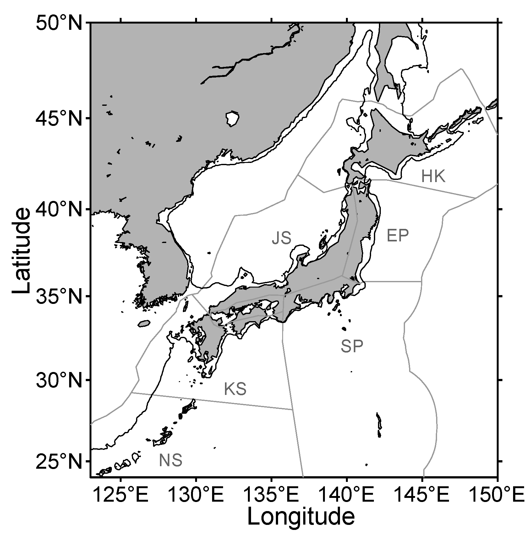
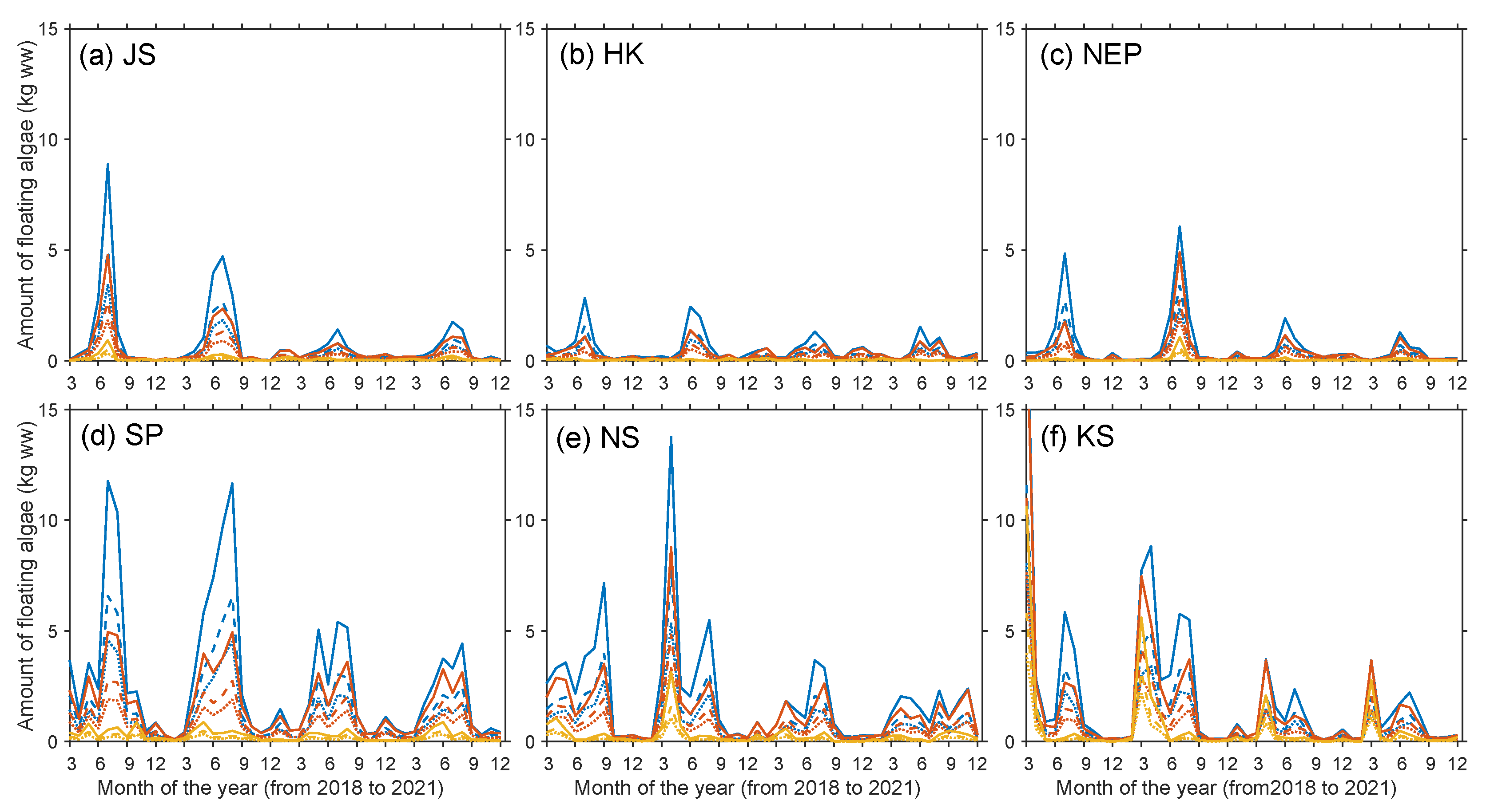
Figure 1. (a) An RGB image (top of atmosphere radiance) acquired by GCOM-C/SGLI (Global Change Observation Mission-Climate/Second-Generation Global Imager) on 2 July 2019. The location is off the coast of Qingdao, China (shown as a red square on the map). (b) Floating algae index (FAI) calculated from GCOM-C/SGLI data collected on the same day and location as in (a). The red-colored area corresponds to the macroalgae patches.
Water 14 03236 g001
Figure 2. An area covered by GCOM-C/SGLI FAI around Japan(123 E–150 E and 23 N–50 N). The 200 m deep isobath is also depicted. The gray line divides the area into subareas, where the macroalgae area is summarized. The subarea is determined based on the subarea divisions by Fisheries Agency, Japan, to establish fishing zones.
Water 14 03236 g002
Figure 3. (a,b): An example of (a) FAI and (b) scaled FAI (sFAI) distribution. Subtracting the adjacent ocean’s FAI from the focal FAI yields sFAI, a scaled-down version of FAI. The main text contains a detailed definition and derivation of sFAI. The data collection took place on 7 May 2019. (c,d): Normalized frequency of the (c) FAI and (d) sFAI distributions in the upper panels.
Water 14 03236 g003
Figure 4. Examples of sFAI images captured on 7 May 2020, in the East China sea by (a) Sentinel-2/MSI and (d) GCOM-C/SGLI. The origin of the axis was located at 125 . 2491 E in longitude and 30 . 4338 N in latitude. Panels (b,c) display the macroalgae area (in m 2 ) in each pixel generated from the sFAI map of panel (a). Macroalgae area was computed using Equation (6), which required upper and lower sFAI thresholds (sFAI max and sFAI min ). In panels (b,c), the identical sFAI max (0.22), but different sFAI min values were used; in (b), sFAI min was the sFAI value at 99.7 % in the cumulative histogram of sFAI, while in (c), sFAI min was at 99.9 % in the cumulative histogram of sFAI. (e,f) were identical to (b,c), except for GCOM-C/SGLI sFAI with the same sFAI max value of 0.0408.
Water 14 03236 g004
Figure 5. Monthly variations in the floating macroalgae area around Japan from 2018 to 2021. The floating macroalgae in all the subareas in Figure 2 were considered. However, macroalgae within four pixels from land (and thus invalid) pixels were excluded.
Water 14 03236 g005
Figure 6. Monthly averaged fractional coverage of floating macroalgae (%; on 0 . 5 × 0 . 5 grids) from GCOM-C/SGLI FAI Japan area product. The color was specified on 1024 levels, and the fractional coverage below 1 × 10 4 % (i.e., 0.1 / 1024 ) remained white.
Water 14 03236 g006
Figure 7. Monthly estimates of the floating macroalgae biomass detected outside continental shelves (deeper than 200 m) in each subarea shown in Figure 2. The colors and line style are identical to those in Figure 5.
Water 14 03236 g007
Table 1. Estimates of floating macroalgae biomass (×10 3 kg wet weight; a total of one year) detected outside continental shelves (deeper than 200 m) in each subarea shown in Figure 2. The values range from the lowest (sFAI min = 99.99% and sFAI max = 0.1) to the highest value (sFAI min = 99.7% and sFAI max = 0.04).
JSHKNEPSPNSKSSum
2018640–14,350250–6750130–93101590–38,8101340–27,6904930–36,8808880–133,790
2019440–13,820230–7030580–11,2501450–42,2201950–32,7303810–34,8508460–141,900
2020350–5640240–6330180–5800950–25,470860–14,8201340–12,3403910–70,380
2021340–5820200–5280210–37201170–19,1801000–16,0501740–11,8204620–61,870
Publisher’s Note: MDPI stays neutral with regard to jurisdictional claims in published maps and institutional affiliations.

